2001 Deliverable Report:
Intelligent Multidimensional Demand Aggregation/Disaggregation Strategies Task 879.001: Intelligent Demand Aggregation and Forecast Solutions
Project 879: Demand Data Mining and Planning in Semiconductor Manufacturing Networks Task Leader: Argon Chen
Co-PI’s: Ruey-Shan Guo and Shi-Chung Chang Students: Chia-Hau Hsu and Yee-Chiu Cheng 1. Abstract and Summary
The demand uncertainty propagated and magnified over the semiconductor demand-supply network is the crucial cause of poor manufacturing/logistic plans. To manage the demand
variability, appropriate demand aggregation/forecasting approaches are known to be
effective. In the first year of this research task, a multivariate time series model is used as a study vehicle to investigate the effect of aggregating interrelated demands. Heuristic demand grouping algorithms, i.e., a variety of Greedy algorithms, are also developed to minimize the safety stock costs under demand uncertainty. The research results provide practitioners practical guidelines and methodologies to select proper aggregation/forecasting approaches and to group demands for minimum safety stock costs.
2. Technical Results
2.1 Aggregation and Forecasting of Interrelated Demands for Operations Planning
An On-Line Analytical Processing (OLAP) tool is useful for analysis of multi-perspective (multi-dimensional) demand aggregation and forecasting. Demand planners can use the tool to quickly roll up demands to an aggregated level for a total demand or drill down a total demand to detailed demands from different perspectives. For example, a semiconductor demand planner can roll up (or aggregate) the detailed demand to calculate the total demand for logic IC in North America and Europe during the first during the last two quarters of the year. The demand planner can also drill down (or disaggregate) the total demand to see, for example, the proportion of the North American market. There are usually three perspectives (dimensions) to view the demands: time, product type, and region. To better understand the natures of certain demands, users of OLAP tools can choose desired perspectives to perform the roll-up and/or drill-down analyses. Demand aggregation/disaggregation is then followed by statistical demand forecasting to further improve the accuracy of demand plans. However, the effect of statistical forecasting is obscure and planners are hesitant to use the pre-determined statistical models because the flawed models often incur more errors and cause poorer forecasts.
This research will use the bivariate vector autoregression (VAR(1)) time series model as a study vehicle to investigate the effects of aggregating two interrelated demands. Performance of corresponding forecasting approaches will be then derived and evaluated. The goal of this research is to use certain statistical properties of the demands to develop principles that can assist the demand planners to determine whether demand aggregation and/or statistical forecasting are needed.
2.1.1 VAR(1) Demand Model and Demand Planning Approaches
In practice, most time-variant demands are observed to follow autoregression time-series models. Particularly, the first order autoregression, AR(1), model is widely applied in both practice and literature (Lee et al., 1997). Since the interrelation of demands is the focal point of our research, the first order bivariate vector autoregression, VAR(1), time series model (Box and Tiao, 1977, Tiao and Box, 1981, and Tiao and Tsay, 1983) is chosen as a study vehicle. Bivariate VAR(1) demands can be denoted as a vector: Xt =
[
X1t,X2t]
′ and the VAR(1) modelcan be expressed as:
t t t u X a X = +Φ −1+ (2.1) where
[
]
′ = ux1,ux2u is the constant vector; = Φ 22 21 12 11 φ φ φ φ
is the autoregression parameter matrix; and
[
]
′= t t
t a a
a 1, 2 is the white noise vector following iid bivariate normal distribution: N2=(0,∑) with
[ ]
′ = 0,0 0 , = ∑ 22 11 0 0 σ σ .In the VAR(1) model, φ 11 and φ 22 represent the
“auto-correlation elements” that dictate how much a demand depends on its own earlier demands; φ12
and φ21 represent the “inter-correlation elements” that
determine how the two demands correlate to each other. In this research, we investigate five possible demand planning approaches in response to the bivariate VAR(1) demands:
(1) Approach 1: The manufacturer lacks the technology of statistical forecasting. Demands are handled as simple time-invariant data sequences. The demand variability is measured by the standard deviation. The safety stock (or production capacity) is planned separately for each demand based on a multiple of its standard deviation.
(2) Approach 2: The manufacturer aggregates the two demands together. The aggregated demand, denoted by Yt (=X1t+X2t), is handled as a
time-invariant data sequence. The safety stock (or production capacity) is planned for two demands together based on a multiple of Yt’s
standard deviation.
(3) Approach 3: The manufacturer owns the statistical forecasting technology but lacks knowledge of multivariate time series. Demands are handled as two independent time series. AR(1) time series models are used as the statistical forecasting models. Statistical forecasting is carried out separately based on the estimated AR(1) time series model for each demand. The safety stock (or production capacity) is planned separately for each demand based on a multiple of its forecast standard error. (4) Approach 4: The manufacturer aggregates the
two demands together. The aggregated demand is handled as an AR(1) time series. The safety stock (or production capacity) is planned for two demands together based on a multiple of the Yt’s
forecast standard error.
(5) Approach 5: The manufacturer owns the technology of forecasting multivariate time series. Statistical forecasting is based on the VAR(1) model. Safety stock (and/or production capacity) is planned separately for each demand based on a multiple of its forecast standard error.
2.1.2 Performance Analysis of Demand Planning Approaches
To analyze and compare the above five approaches, theorems are developed to understand the properties of the time series aggregated from VAR(1) time series.
Theorem 2.1:
If X1t and X2t follow VAR(1) model in (2.1), then X1t can be expressed as V1t+V2t where V1t and V2t are two AR(1) time series. Similarly, X2t can be expressed as W1t+W2t where W1t及W2t are two AR(1) time series.
Theorem 2.2:
D1t and D2t are two stationary AR(1) time series.
Let Dt be the sum of D1t and D2t, i.e.
t t
t D D
D = 1 + 2. Suppose that Dt is thought to be
an AR(1) time series, i.e.,Dt =uD+ϕaDt−1+εt. The expected maximum likelihood estimate of
φa and
σ
ε2 are derived and formulas areprovided. Corollary 2.1:
X1t and X2t follow the AR(1) model in (2.1). If Yt
is the sum of X1t and X2t, then Yt can be
expressed as U1t+U2t where U1t and U2t are two AR(1) time series.
2.1.3 Evaluations and Suggestions of Demand Planning Approaches
With the understanding of the aggregated time series in the previous section, five demand planning approaches can be now analytically evaluated and compared. Overall, we have the following observations based on evaluation and comparison results.
a. With aggregation and statistical forecasting capabilities, Approach 4 appears to be the best approach regardless of the scenarios. Approach 4’s effetiveness is also the most stable and less affected by changes of demand correlation and ratio of variation sizes.
b. The simple aggregation approach, Approach 2, performs quite as good as Approach 4 and outperforms Approach 5, the most sophisticated statistical forecasting approach, when the demand correlation is weak or negative. Its performance, however, worsens quickly as the demand correlation becomes positive and large and the two variation sizes become significantly different. c. Approach 3, even with its statistical forecasting
capability, appears to be the worst approach. It outperforms Approach 2 only in Scenario 1 when two demands are more positively correlated and the variations sizes are different.
Now, we summarize our observations and provide the following principles and guidelines for practitioners to adopt appropriate demand planning approaches under different situations.
(1) Demand correlation is negative (ρ < 0)
a. If aggregating demands only incurs a limited extra cost, Approach 2 appears to be the best choice since it requires only simple aggregation and does not need to build statistical model for forecasting.
b. If demand aggregation will incur a substantial extra cost, Approach 5 should be adopted. However, Approach 5 requires a correct multivariate statistical model for accurate forecasts. When the demand correlation is insignificant but individual demands have significant autocorrelations, Approach 3 is a good choice for making more than 10% cost reduction.
(2) Demand correlation is positive (ρ > 0)
a. If the correlation is low, 0<ρ <0.2, and the extra aggregation cost is minimum, Approach 2 is still a good choice given that no statistical model is required for this approach.
b. If the correlation is high, ρ >0.2, and the extra aggregation cost is limited, Approach 4 is more preferable. It should be noted that building a univariate time series model for an aggregated demand in Approach 4 is much more reliable and simpler than building the multivariate time series model in Approach 5.
c. If the extra aggregation cost is substantially large, Approach 5 has to be adopted. Again, Approach 3 can be used instead when low demand correlation and high autocorrelation are observed.
2.2 Aggregation Strategies to Minimize Safety Stock Costs Under Uncertain Demands
In this research, base on the inventory cost of (s,S) policy, we develop heuristic aggregation strategies to find combinations of multiple demand sources that achieve maximum cost saving.
2.2.1 Inventory cost model under random demand
In this research, inventory cost model is established based on (s,S) policy. Within each time unit, demands would consume the inventory. When the inventory level reaches exactly at the reorder point, replenishment is made. During this replenishment time, demands would continue to occur. However, the quantity of the demand per unit time is not in a fixed number, it cannot be known that how much quantity a customer would order before the transaction occurred. Based on the above assumptions, notations are defined as follows,
1. AVG: average demand per unit time
2. STD: standard deviation of demand per unit
time
3. L: replenishment lead time
4. K: ordering cost (setup cost)-a constant
5. h: unit holding cost, i.e. cost of holding one
unit inventory for one unit time
6. δ: stocking out probability; i.e., service level=(1−δ)×100%
7. c: unit inventory cost, i.e., cost of one
product unit The inventory cost becomes
STD L cz h AVG K c 2 2 + where δ − = + ≥ 1 } 2 2 1 time lead during demand { z LSTD h AVG K P
Consider 2 customer zones (demand sources) that can be served by two local distributors or by a single centralized distributor. Let α be the ratio of the centralized distributor lead-time to the local distributor lead-time; u be the ratio of the expected number of demand 1 to the expected number of demand 2; and v be the ratio of the standard deviation of demand 1 to the standard deviation of demand 2. Then the safety stock cost reduction percentage
function (CR%): % 100 1 2 1 1 2 × + + + − + v v v v α ρ
is used as the demand grouping criterion. 2.2.2 Greedy algorithm
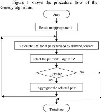
Figure 1 shows the procedure flow of the Greedy algorithm.
Start
Calculate CR for al l pairs formed by demand sources
Select the pair with largest CR
CR>0?
Aggregate the selected pair
Terminate Yes
No Select an appropriate α
Figure 1 Flow of the Greedy algorithm
Theorem 2.3: Optimality conditions of the Greedy algorithm for n demand sources combinations
If the optimal solution has separated aggregate groups that:
a. any pair within an aggregate group has a positive CR, (CR>0); and
b. any pair formed by members from different aggregate groups has a negative
CR, (CR≤0);
then, the solution provided by the Greedy algorithm would be optimal.
2.2.3 Grasping algorithm
Figure 3 shows the procedure flow of the Grasping algorithm.
Start
Pairing demand sources Calculate CR for each pair
Aggregate the pair with maximum CR>0 Let say the pair ( a p, a q)
None CR>0 ?
Cancel the pairs containing a or p a q
None CR>0 ? Terminate Yes No Yes No Select an appropriate α
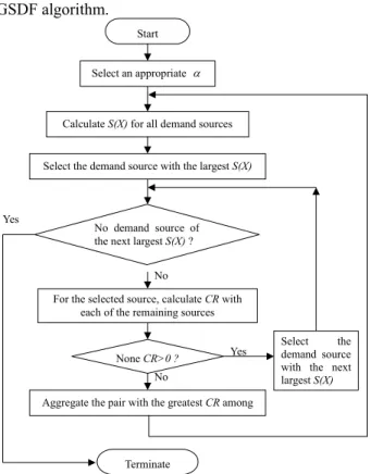
Figure 3 Flow of the Grasping algorithm 2.2.4 Greatest Standard Deviation First (GSDF) algorithm
Figure 4 shows the procedure flow of the GSDF algorithm.
Start
Calculate S(X) for all demand sources
Select the demand source with the largest S(X)
For the selected source, calculate CR with each of the remaining sources
None CR>0 ?
Select the demand source with the next largest S(X) No demand source of
the next largest S(X) ? Yes
No
Yes
Terminate No
Aggregate the pair with the greatest CR among Select an appropriate α
Figure 4 Flow of the Greatest Standard Deviation First (GSDF) algorithm
2.2.5 Case study and summary of demand-grouping algorithm performances
In this section, a set of real demand data from a semiconductor manufacturing firm is used for the verification and further evaluation of algorithms that has mentioned in the previous sections. The data is in spreadsheet format (Microsoft Excel). The algorithms are coded in VBA (Visual Basic for Application). The performances of proposed demand grouping algorithms are evaluated and compared.
Some suggestions and guidelines are given for applying the proposed algorithms:
1. In the case study, the Greedy algorithm seems to give a pretty good performance both in the optimality and the computing efficiency. However, the computing efficiency is drastically worsened as the number of demand sources increases. It is because as the number of demand sources increases, the total number of pairing increases. Hence, the Greedy algorithm is best to use when the number of demand sources is not too large.
2. The computing efficiency of the Grasping algorithm is better than other algorithms especially when the number of demand sources is large. It is because the Grasping aggregate more than once for each stage of pairings. Thus, the Grasping algorithm is the best to use when a high efficiency of computing the combinatorial solution is required.
3. The Greatest Standard Deviation First (GSDF) algorithm is worse than the other algorithms in the optimality because of the constraint on the size of the demand standard deviation. But, it may be appropriate to use when some targets of demand sources with large variability are pre-determined. These targets will be ch
Researches on aggregation strategies for other cost models, such as capacity cost model, will be further carried out in the future research.