An Efficient Data Reporting Scheme in Large Wireless Sensor Networks with Mobile Sinks

An Efficient Data Reporting Scheme in Large Wireless Sensor

Networks with Mobile Sinks

Shiow-Fen Hwang, Kun-Hsien Lu, Yun-Shen Wang, Yi-Yu Su, Chyi-Ren Dow

Department of Information Engineering and Computer Science

Feng Chia University, Taichung, Taiwan 40724, R.O.C.

Email: {sfhwang, p9217988, m9433201, p9112089, crdow@fcu.edu.tw}

Abstract

-Efficient data reporting is an important

issue for wireless sensor networks (WSNs) with mobile sinks. However, high sink update cost causes sensor nodes to consume much energy, especially when sinks move rapidly. In this paper, we propose an efficient data reporting scheme in large WSNs with mobile sinks. In our network environment, the sensor field is divided into several grids, and forms a hierarchical sensor network adaptively, according to network sizes. We set location servers to provide the location information of the mobile sink. Only those sensor nodes in a small area where the mobile sink is located need to construct weight function to find an efficient path to the mobile sink. Therefore, energy consumption caused by location update cost from the mobile sink is significantly reduced. Meanwhile, we dynamically adjust the update scope according to the location of the mobile sink, to further reduce the energy consumption. Simulation results show that our proposed method is scalable, and outperforms TNT and our previous work[9], in terms of average energy consumption per round and successful rate.

Keywords: wireless sensor networks, data

reporting, hierarchical, mobile sink, grid.

1. Introduction

A wireless sensor network (WSN) is composed of one or several sinks (base stations), and a large number of sensors. Sensor nodes have limited capacities, such as power supply, computing ability, and memory storage,…, etc., and are responsible for sensing and forwarding the specific data to the sink[1]. Therefore, WSNs are relegated as application or task oriented networks.

Data gathering is a basic and important operation in WSNs. It can be categorized into three methods including time-driven, event-driven, and query-driven [2]. In these methods, sensor nodes

near to the sink usually consume more energy to deliver data than sensor nodes far from the sink and the network lifetime suffers from the hotspot problem when the sink is stationary. Recently, a number of proposed studies [3-7] showed that mobile sinks can provide lots of advantages over static sinks. For example, a mobile sink can redirect traffic flows and balance the energy consumption among sensor nodes. However, in such scenario that the mobile sink moves arbitrarily in the sensor field, how to design an efficient data reporting scheme for sensor nodes is a critical issue.

In [8], Q.Ye et al. have proposed two protocols, called TNT and PTNT, to address sink mobility problem. In TNT, each node maintains a tracking counter and sets up a beacon timer. The mobile sink broadcasts a beacon periodically to its neighboring nodes. If a neighboring node receives the beacon, then increases its tracking counter by 1, otherwise, decreases that by 1 when the beacon timer expires. Therefore, the sensed data can be forwarded to the mobile sink by using the sequence of the tracking counters. However, in this scheme, inefficient paths could be incurred due to the special movement patterns of the sink, thus result longer transmission delays.

S.-F. Hwang et al. [9] proposed a weight function to provide efficient data reporting in WSNs with mobile sinks. Sensor field is divided into several grids and only one node is selected as a head in each grid. For saving energy, some heads become active nodes to sense and forward data in each round. The definition of a round is, the mobile sink issues a query to request active nodes to sense and gather the queried data, and the sink moves arbitrarily until it receive the gathered data. In addition, all active nodes are classified into multiple levels. The classified levels are utilized to construct the weights of active nodes, according to the weight algorithm in [9]. When the active nodes receive a query from the mobile sink, the queried information can be forwarded along the path

determined by the active nodes’ weights. When the mobile sink moves, it only needs to locally broadcast an update packet to its neighboring active nodes, and the classified levels are used to limit weight update scope. However, this method can not scale well to large sensor networks, the main reason is that the location update scope becomes very large, and the frequent location updates consume much energy.

In this paper, we propose a scalable method to improve the method proposed in [9]. Our proposed method is based on [9], the differences are that we divide the sensor network into several blocks adaptively to form a hierarchical sensor network. Only sensor nodes in the block where the mobile sink is located need to construct multiple levels and weights information. Therefore, the update scope is limited to a block. Furthermore, we propose a dynamic update method to adjust the update scope dynamically, according to the location of the mobile sink.

The rest of this paper is organized as follows. Section 2 introduces the network model. Section 3 describes efficient data reporting. Section 4 summarizes simulation results. The conclusion is in Section 5.

2. Network Model

Let a sensor network be partitioned into 2n_×2n

grids, and the coordinate of a node is the coordinate of the grid that it is located in.

The node with the smallest ID in a grid will first serve as the head. Other nodes in the grid enter to sleep mode for conserving energy. In addition, some heads are designated to be active nodes and other heads enter to sleep mode according to the active node selection algorithm proposed in [9]. Figure 1 displays two examples of the selected active nodes by using the active node selection algorithm.

For the communication of two adjacent active nodes, the transmission range is defined as 2 2 d, where d is the length of the grid side. For good coverage, the sensing range is defined as 5d.

(a) round r (odd) (b) round r+1 Figure 1. Active nodes in round r and round r+1.

In order to manage the network efficiently, the

network is partitioned into different layers in advance as follows.

A grid is called a layer-0 grid. A layer-1 grid is composed of 2r_×2r _{layer-0 grids, r}≥_{1. (For}

convenience, a layer-1 grid is called a block later). A laye-2 grid is composed of 2×2 layer-1 grids, and a layer-i grid is composed of 2×2 layer-(i-1) grids, i=2, ,L n r− +1.

Let a node p with coordinate( , )x y_{0 0} , then its coordinate in the block where it located is

(

0 0

)

( ', ')x y = x mod 2 ,r y mod 2r , (1) and its coordinate of layer- i is

(

_,

)

0 _, 0 _{, 1, 2, , 1} 1 1 2 2 i i x y x y i n r r i r i ⎛⎢ ⎥ ⎢ ⎥⎞ =⎜_⎜⎢ _{+ −} ⎥ ⎢ _{+ −} ⎥⎟_⎟ = − + ⎣ ⎦ ⎣ ⎦ ⎝ ⎠ L (2) Figure 2 shows an example of a 2 layers sensor network, where r=2, n=3. The original coordinate of A is (5,6), the coordinate of A in its block is (1,2), and the coordinates of A in layer-1 and layer-2 are (1,1) and (0,0), respectively.

(0,0) (1,0)(2,0)(3,0)(4,0) (5,0) (6,0) (7,0) A (0,1) (1,1)(2,1)(3,1)(4,1) (5,1) (6,1) (7,1) (0,2) (1,2)(2,2)(3,2)(4,2) (5,2) (6,2) (7,2) (0,3) (1,0)(2,3)(3,3)(4,3) (5,3) (6,3) (7,3) (0,4) (1,4)(2,4)(3,4)(4,4) (5,4) (6,4) (7,4) (0,5) (1,5)(2,5)(3,5)(4,5) (5,5) (6,5) (7,5) (0,6) (1,6)(2,6)(3,6)(4,6) (5,6) (6,6) (7,6) (0,7) (1,7)(2,7)(3,7)(4,7) (5,7) (6,7) (7,7) Y X A (0,0) (1,0)(2,0)(3,0) (0,1) (1,1)(2,1)(3,1) (0,2) (1,2)(2,2)(3,2) (0,3) (1,3)(2,3)(3,3) (0,0) (1,0)(2,0)(3,0) (0,1) (1,1)(2,1)(3,1) (0,2) (1,2)(2,2)(3,2) (0,3) (1,3)(2,3)(3,3) (0,0) (1,0)(2,0)(3,0) (0,1) (1,1)(2,1)(3,1) (0,2) (1,2)(2,2)(3,2) (0,3) (1,3)(2,3)(3,3) (0,0) (1,0)(2,0)(3,0) (0,1) (1,1)(2,1)(3,1) (0,2) (1,2)(2,2)(3,2) (0,3) (1,3)(2,3)(3,3) Y X (1,1) (0,0) (a) (b) Figure 2. (a) Original coordinates, (b) The

coordinates of A in layer-1 and layer-2. Those active nodes which are closest to the center in each layer-i grid are chosen as location servers of layer-i, i≥2. They record the location information about the mobile sink. If the coordinates of the mobile sink in layer-i is( ,

x y

_{i i}),

then its location server of layer-i stores the

location information of the mobile sink as

sink_loc(sink_id,( ,

x y

_{i i})) in its location table.

3. Efficient Data Reporting

In this section, we describe the proposed efficient data reporting scheme, including the classification of active nodes, the construction of local weights, the dynamic update method and data forwarding. The main goal of our scheme is to reduce the energy consumption and support good scalability as well.

3.1 Classification of active nodes

balance the energy consumption among active nodes. First, all active nodes are classified into two levels, level 1 and level 2, by using the active node level classification algorithm proposed in [9], as shown in Figure 3. Therefore, an active node p can determine whether it belongs to level 1 or level 2 in round r, and sets up its low level value L(p). After the active node p knows its L(p) (i.e. equal to 1 or 2) in a given round, then its highest level value L'(p) will be defined in advance.

ActiveNodeLevelClassification(r, ) if ( mod 2 = 0 and r mod 4 = 0 or 1) or

( mod 2 = 1 and r mod 4 = 2 or 3) then

L(p)=1 else L(p)=2 end if ' x ( ', ') p= x y ' x

Figure 3. Active node level classification algorithm.

The following definition 1 is used to find the highest level of the active node p.

Definition 1. For an active node p, if its four

(diagonal) neighboring active nodes exist and all of them belong to level i (i≧2), then the active node p belongs to level (i+1). The highest level of an active node is the maximum value of the level which it belongs to.

By definition 1, active node p can know which levels it belongs to by locally communicating with its neighboring active nodes, and active node p can find its L'(p). We observe that the active node will be closest to the center of the sensor field if its highest level value is maximum.

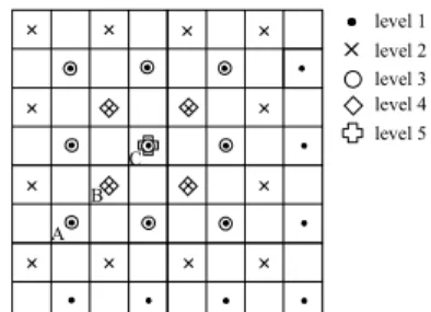
Figure 4 shows an example of the classified level in a 8×8 (grids) networks. First, level 1 active node A has four neighboring level 2 active nodes, thus node A belongs to level 3. Then, level 2 active node B has four neighboring level 3 active nodes, node B belongs to level 4. Final, level 3 active node C knows that it also belongs to level 5

in the same way. Consequently, we have L(A)=1,

L' (A)=3, L(B)=2, L' (B)=4, L(C)=1, and L' (C)=5. level 1 level 2 level 3 level 4 level 5 A B C

Figure 4. Levels of some active nodes in a block.

3.2. Construction of local weights

When the mobile sink executes a task, it first

issues a Sink Query Packet (SQP), and then

broadcasts it to all active nodes. The SQP format is Sink_Query <sink_id, type, weight, round>, where

the type field represents the role of the active node

sending the SQP packet, the round field means

current round number. The type values is 0, 1, or 2, which indicates the mobile sink, level 1 active node, or level 2 active node, respectively. Each active node receiving the SQP packet builds its low level weight w, and highest level weight w'.

The w and w' are utilized to forward data during

data reporting.

An active node p receiving the SQP packet for the first time determines if it should rebroadcast the SQP packet or not, and then sets up its low level weight according to the weight construction algorithm in [9]. Figure 5(a) shows an example of low level weight construction, the number displayed in the bottom-right corner of each grid indicates w. We can observe that an active node far away from the sink will have larger w than those which are near to the sink. After the active node p obtains its w(p), it use (3) to calculate w'(p). Figure 5(b) is an example of highest level weight (w') construction, the number displayed in the bottom-right corner of each grid indicates w and the other number displayed in the upper-right corner of each grid indicates w'. Note that only the active nodes in the block including the sink need to construct the weight values. If an active node needs to transmit data packet to the sink, it just needs to query its nearest location server to get the location of the block which the sink is located in.

'( ) ( ) '( ) max{ ( ) ( ),0} 2 L p L p w p = w p − −

(3) 0 1 2 3 0 1 2 3 1 1 2 3 1 1 2 3 2 2 2 2 2 2 3 3 3 3 3 3 3 3 3 3 0 0 0 1 2 2 2 1 2 1 2 1 2 0 1 2 3 0 1 2 3 1 1 2 3 1 1 2 3 2 2 2 2 2 3 3 3 3 3 3 3 3 3 3 2 S S

(a) (b)

Figure 5. (a) An example of low level weight (w) construction. (b) An example of highest level weight (w') construction. Note that some grids do not be labeled w' values, it means that w' is equal

to w.

While the mobile sink just moves in a block, only some of the active nodes in the block need to update their weights according to the weight update algorithm in [9], as shown in Figure 7.

However, when the mobile sink moves to a neighboring block, it will broadcast and construct the highest level value and weight values in the new block. The active nodes in the old block will keep the weight values for a while, until the border nodes of the old block do not sense the mobile sink. Figure 6 shows an example that a mobile sink moves to a neighboring block, it broadcasts an announcement packet to active nodes in the new block, active nodes receiving the packet construct their highest level value and weight values.

0 1 2 3 0 1 2 3 1 1 2 3 1 1 2 3 2 2 2 2 2 2 3 3 3 3 3 3 3 3 3 3 0 0 0 1 2 2 2 1 2 1 2 1 2 S

Figure 6. A mobile sink moves to a neighboring block.

WeightUpdate (Sink_Beacon<sink_id, type, i>)

An active node receives a sink beacon packet

if L'(p)≧i then

if (type =0 and L(p)=1) or (type =1 and L(p)=2) or

(type =2 and L(p)=1) then

w'(p)=0 i=i+1 type= L(p)

broadcast sink beacon packet

end if end if

Figure 7. Weight update algorithm.

3.3 Dynamic update method

According to the weight values, we can find an efficient path to forward data to the mobile sink. However, when the mobile sink moves, weight information must be updated. Figure 7 is the weight update algorithm which proposed in [9], where i is used to limit the update scope, and its initial value is 1. The mean of the type is the same as in SQP packet. In this algorithm, an active node p receiving the sink beacon packet resets its w'(p) as 0, and increases i value by 1 to rebroadcast. It is obvious that a method for reducing weight update cost is to increase the increment of i value. For example, i = i + 1 can be simply modified as i = i +

β, where β=1, 2, 3, …. Hence, the larger the β value is, the smaller the update scope is. However, this method is inflexible.

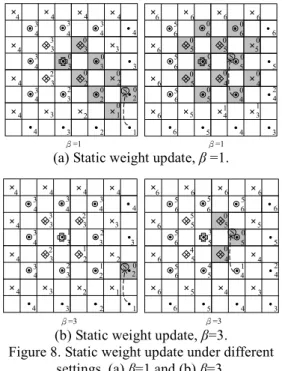
When the mobile sink is in the corner of a block, and the β value is set as 1 (Figure 8(a)), the update cost is not very high and the effect on hop counts is not obvious. However, the update cost becomes very high while the sink moves to the center of a block. If the β value is set as 3 (Figure 8(b)), when the mobile sink is in the corner of a block, the update scope is too small to effect on the hop counts and the successful rate of data packets may decrease. However, when the sink is in the center of a block, since the active nodes reach the center of the sensor network easily according to the weight values of active nodes. Therefore, the sink update scope can be small and do not effect on the hop count and the successful rate of data packet.

For avoiding the disadvantage of fixing β, we propose a dynamic update method to improve the energy efficiency and preserve the successful rate of data packet. We adjust the parameter of dynamic scope, β, according to the location of the mobile sink in a block. The algorithm is shown in Figure 9. 1 2 3 4 1 2 3 4 2 2 3 4 2 2 3 4 3 3 3 3 3 3 4 4 4 4 4 4 4 4 4 4 0 0 0 0 3 3 3 2 3 0 3 2 3 S 0 0 0 β=1 β=1 3 4 5 6 3 4 5 6 4 4 5 6 4 4 5 6 5 5 5 5 5 5 6 6 6 6 6 6 6 6 6 6 0 0 0 0 0 5 5 0 0 0 0 0 5 S 2 0 1 0 1

(a) Static weight update, β =1.

1 2 3 4 1 2 3 4 2 2 3 4 2 2 3 4 3 3 3 3 3 3 4 4 4 4 4 4 4 4 4 4 1 1 1 2 3 3 3 2 3 2 3 2 3 S 0 β=3 β=3 3 4 5 6 3 4 5 6 4 4 5 6 4 4 5 6 5 5 5 5 5 5 6 6 6 6 6 6 6 6 6 6 1 0 3 0 5 5 5 4 5 0 5 4 5 S 2

(b) Static weight update, β=3. Figure 8. Static weight update under different

settings, (a) β=1 and (b) β=3. 2r DynamicUpdate( , a , b , k, ) then β=a else β=b end if sink( , )x ys s if ( 2r (1 ) 2 rand 2r y (1 ) 2 )r s s k× ≤ x ≤ − ×k k× ≤ ≤ − ×k

Figure 10. An example of the setting of β. 1 2 3 4 1 2 3 4 2 2 3 4 2 2 3 4 3 3 3 3 3 3 4 4 4 4 4 4 4 4 4 4 0 0 0 0 3 3 3 2 3 0 3 2 3 S 0 0 0 3 4 5 6 3 4 5 6 4 4 5 6 4 4 5 6 5 5 5 5 5 5 6 6 6 6 6 6 6 6 6 6 1 0 3 0 5 5 5 4 5 0 5 4 5 S 2 (a) (b)

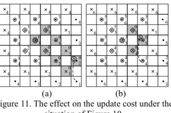
Figure 11. The effect on the update cost under the situation of Figure 10.

If the mobile sink is nearer to the center than to the border, β is set as a, otherwise, β is set as b, where a > b. Figure 10 is an example of the setting

of β, where value k is set as 1/4, value a is 3 and

value b is equal to 1. Figure 11 indicates the effect on the update cost under the situation of Figure 10, in (a), since the mobile sink is near to the border of the block, the value of β is set as 1, and when the mobile sink moves to near the center as in (b), the value of β is adjusted dynamically to be 3.

3.4 Data forwarding

When an active node p needs to send data packet to the mobile sink s, there are two situations:

(a) p and s are in the same block: First, active node p transmits a data packet to a neighboring active node n which has the smallest w'. If there are two or more neighboring active nodes with the same w', the active node p randomly selects one of them to transmit. Gradually, the data packet will be transmitted to an active node which w' is equal to zero. And then, this active node continuously forwards the data packet along the path that the active nodes which w' are zero, until reach to the mobile sink. Figure 12 shows an example of data forwarding where P1 and s are in a same block.

(b) p and s are in different blocks: The active node p queries the location information of s from the nearest location server, and employs a greedy routing to forward the data packet to the block where the mobile sink is located. Then, the data packet will be transmitted to the mobile sink as situation (a). Figure 13 shows an example of data

forwarding where P2 and s are in different blocks.

Node P2 gets the location of the block which s is

located in from its nearest location server, and then successfully forwards the data packet to the mobile sink s. 0 1 2 3 0 1 2 3 1 1 2 3 1 1 2 3 2 2 2 2 2 2 3 3 3 3 3 3 3 3 3 3 0 0 0 1 2 2 2 1 2 1 2 1 2 S P1

Figure 12. Data forwarding in a same block.

0 1 2 3 0 1 2 3 1 1 2 3 1 1 2 3 2 2 2 2 2 2 3 3 3 3 3 3 3 3 3 3 0 0 0 1 2 2 2 1 2 1 2 1 2 S 2 P

Figure 13. Data forwarding in different blocks.

4. Simulation Results

In the simulation environment, the entire sensor network is divided into 8×8, 16×16, 32×32 and 64×64 grids with 400, 800, 3200 and 6000 sensor nodes, respectively. The side length of each grid is 12.5m. We set a block size is 8×8 grids. The first order radio model proposed in LEACH[10] is used to calculate the energy consumption of a sensor node. The size of a data packet is 2000 bits and the size of a control packet is 64 bits. A mobile sink with speed 10m/s is deployed and the sink beacon interval varies from 1 to 6 seconds. We compare the proposed dynamic update method to our previous method [9] and TNT [8]. In [9], it requests the mobile sink to locally broadcast a weight update packet and uses a constant β value to limit the flooding scope of the update packet. Therefore, we abbreviate this method to be “static update”. On the other hand, in our proposed

dynamic update method, β value is dynamically

changed according to the location of the mobile sink in the block as shown in Figure 9 so that we

present β value as (b,a) in the following simulation results. Three performance metrics including average energy consumption per round, average hop counts, and successful rate are evaluated. The successful rate indicates the ratio of the number of data packets successfully received by the mobile sink to the total number of data packets sent by active nodes. 0 0.002 0.004 0.006 0.008 0.01 1 2 3 4 (1,2) (1,3) (1,4) (2,3) (2,4) (3,4) β Av er ag e po w er c ons um pt io n pe r ro un d ( J) 1 2 3 4 (1,2) (1,3) (1,4) (2,3) (2,4) (3,4)

(a) Network size: 8×8 grids

0 0.03 0.06 0.09 0.12 0.15 1 2 3 4 (1,2) (1,3) (1,4) (2,3) (2,4) (3,4) β Av er ag e po w er c on su m pt io n pe r ro un d ( J) 1 2 3 4 (1,2) (1,3) (1,4) (2,3) (2,4) (3,4)

(b) Network size: 16×16 grids

0 0.005 0.01 0.015 0.02 0.025 0.03 0.035 0.04 1 2 3 4 (1,2) (1,3) (1,4) (2,3) (2,4) (3,4) β Av er ag e p ow er c on su m pt io n pe r ro und ( J) ₁ 2 3 4 (1,2) (1,3) (1,4) (2,3) (2,4) (3,4)

(c) Network size: 32×32 grids

0 0.1 0.2 0.3 0.4 0.5 0.6 0.7 0.8 1 2 3 4 (1,2) (1,3) (1,4) (2,3) (2,4) (3,4) β Av er age p ow er c on su m pt io n pe r r ou nd ( J) 1 2 3 4 (1,2) (1,3) (1,4) (2,3) (2,4) (3,4)

(d) Network size: 64×64 grids Figure 14. Average energy consumption under

different update scope settings.

Figure 14 shows that the average energy consumption per round for different β values under different network sizes. In the proposed dynamic update method, the sensor network is partitioned into several blocks, and a small number of location servers are selected to store the sink’s location information. Meanwhile, in the block where the sink is located, the dynamic update method is utilized to reduce the weight update cost incurred by sink mobility. Therefore, it has less average energy consumption than the static update scheme, especially when the network size is large. Figure

15 shows that the successful rate for different β values under different network sizes. The dynamic update method can keep high successful rate while reducing the average energy consumption per round.

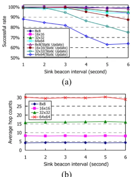
Figure 16 shows the successful rate and average hop counts under different network sizes and sink beacon intervals. The β values for dynamic update and static update method are set as (2,3) and 1, respectively. The results indicate that the dynamic update method has at least 90% successful rate even in high sink beacon intervals and large network sizes while the successful rate of the static update method decreases rapidly in the same environment. Moreover, in Figure 16(b), average hop counts of the dynamic update method do not be affected under different sink beacon intervals. Figure 17 shows the comparison of the dynamic update method, the static update method, and TNT. The results indicate that TNT has higher average hop counts than other methods and the dynamic update method has less energy consumption per round than other methods.

50% 60% 70% 80% 90% 100% 1 2 3 4 (1,2) (1,3) (1,4) (2,3) (2,4) (3,4) β Su cce ss fu l r at e ( % ) 1 2 3 4 (1,2) (1,3) (1,4) (2,3) (2,4) (3,4)

(a) Network size: 8×8 grids

50% 60% 70% 80% 90% 100% 1 2 3 4 (1,2) (1,3) (1,4) (2,3) (2,4) (3,4) β Su cc es sf ul ra te ( % ) 1 2 3 4 (1,2) (1,3) (1,4) (2,3) (2,4) (3,4)

(b) Network size: 16×16 grids

50% 60% 70% 80% 90% 100% 1 2 3 4 (1,2) (1,3) (1,4) (2,3) (2,4) (3,4) β Su cc essf ul ra te ( % ) 1 2 3 4 (1,2) (1,3) (1,4) (2,3) (2,4) (3,4)

(c) Network size: 32×32 grids

50% 60% 70% 80% 90% 100% 1 2 3 4 (1,2) (1,3) (1,4) (2,3) (2,4) (3,4) β Su cce ss fu l r at e ( % ) 1 2 3 4 (1,2) (1,3) (1,4) (2,3) (2,4) (3,4)

(d) Network size: 64×64 grids

Figure 15. Successful rate under different update scope settings.

50% 60% 70% 80% 90% 100% 1 2 3 4 5 6

Sink beacon interval (second)

Su cce ss fu l r at e 8x8 16x16 32x32 64x64 8x8(Static Update) 16x16(Static Update) 32x32(Static Update) 64x64(Static Update) (a) 0 5 10 15 20 25 30 1 2 3 4 5 6

Sink beacon interval (second)

Av er ag e h op c ou nt s _8x8 16x16 32x32 64x64 (b)

Figure 16. (a) Successful rate, (b) Average hop counts under different network sizes and sink

beacon intervals. 0 10 20 30 40 50 8x8 16x16 32x32 64x64

Network size (grids)

Ave ra ge ho p c oun ts TNT_{Static update} Dynamic update (a) 0 0.4 0.8 1.2 1.6 2 8x8 16x16 32x32 64x64

Network size (grids)

A ve rage po we r co ns umpt io n p er r ou nd(J ) TNT Static update Dynamic update (b)

Figure 17. (a) Average hop counts, (b) Average energy consumption per round under different

network sizes.

5. Conclusion

In this paper, we propose an efficient data reporting scheme in large wireless sensor networks with mobile sinks. We build a hierarchical sensor network to alleviate the energy consumptions of active nodes. Only the block where the mobile sink is located need to construct level and weight information, and provides an efficient reporting path to the mobile sink. We also propose the dynamic update method to reduce update cost in advance when the mobile sink moves. Simulation

results show that our proposed method is scalable, and outperforms TNT and our previous work[9], in terms of average energy consumption per round and successful rate.

Acknowledgement

This research is supported by the National Science Council of the Republic of China under grant number NSC-96-2628-E-035-074-MY2.

References

[1] I.F. Akyildiz, W. Su, Y. Sankarasubramaniam, and E. Cayirci, “Wireless sensor networks: a survey,”

Computer Networks, vol. 38, no. 4, pp. 393–422,

2002.

[2] J.N. Al-Karaki and A.E. Kamal, “Routing techniques in wireless sensor networks: a survey,” IEEE

Transactions on Wireless Communications, vol. 11,

no. 6, pp. 6–28, 2004.

[3] J. Luo and J.-P. Hubaux, “Joint mobility and routing for lifetime elongation in wireless sensor networks,”

Proceedings of IEEE INFOCOM, pp. 1735–1746,

2005.

[4] Yanzhong Bi, Jianwei Niu, Limin Sun, Wei Huangfu, and Yi Sun, “Moving Schemes for Mobile Sinks in Wireless Sensor Networks,” Proceedings of IEEE

IPCCC, pp.101–108, 2007.

[5] Yanzhong Bi, Limin Sun, Jian Ma, Na Li, Imran Ali Khan, and Canfeng Chen, “HUMS: an autonomous moving strategy for mobile sinks in data-gathering sensor networks,” Journal on Wireless

Communications and Networking, 2007.

[6] Z. Vincze, R. Vida, and A. Vidács, “Deploying Multiple Sinks in Multi-hop Wireless Sensor Networks,” Proceedings of IEEE International

Conference on Pervasive Services, pp. 55–63, 2007.

[7] Gaotao Shi, Minghong Liao, Maode Ma, and Yantai Shu, “Exploiting sink movement for energy-efficient load-balancing in wireless sensor networks,”

Proceeding of the ACM international workshop on Foundations of wireless ad hoc and sensor networking and computing, pp. 39–44, 2008.

[8] Q. Ye and L. Cheng, “A Lightweight Approach to Mobile Multicasting in Wireless Sensor Networks,”

International Journal of Ad Hoc and Ubiquitous Computing, vol. 2, no. 1/2, pp. 36–45, 2007.

[9] S.-F. Hwang, K.-H. Lu, L.-R. Yang, and C.-R. Dow, “Efficient Data Reporting for Object Tracking in Wireless Sensor Networks with Mobile Sinks,”

Proceedings of The 14th Asia-Pacific Conference on Communications (APCC), 2008.

[10]W.R. Heinzelman, A. Chandrakasan, and H. Balakrishnan, “Energy-Efficient Communication Protocol for Wireless Microsensor Networks,”

Proceeding of the 33rd Hawaii International Conference on System Sciences, 2000.