應用於正交分頻多工系統之框碼同步方法及其效能評估

全文

(1)國立交通大學電信工程學系碩士班碩士論文應用於正交分頻多工系統之框碼同步方法及其效能評估 Frame Synchronization Techniques and Performance Evaluation for OFDM-Based Systems. 研究生：詹克偉指導教授：李程輝教授. 中華民國九十三年六月.

(2) 應用於正交分頻多工系統之碼框同步方法及其效能評估 Frame Synchronization Techniques and Performance Evaluation for OFDM-Based Systems 研究生：詹克偉指導教授：李程輝教授. Student: Ke-Wei Jhan Advisor: Prof. Tsern-Huei Lee. 國立交通大學電信工程學系碩士班碩士論文. A Thesis Submitted to Institute of Communication Engineering College of Electrical Engineering and Computer Science National Chiao Tung University in Partial Fulfillment of the Requirements for the Degree of Master of Science in Communication Engineering June 2004 Hsinchu, Taiwan, Republic of China.. 中華民國九十三年六月.

(3) 應用於正交分頻多工系統之框碼同步方法及其效能評估研究生：詹克偉. 指導教授：李程輝教授. 國立交通大學電信工程學系碩士班. 中文摘要. 在現今高速傳輸的通訊系統當中，正交分頻多工 (OFDM) 技術因其有效使用頻寬以及抵抗多重路徑干擾的特性而受到重視。 OFDM 系統的主要問題在於時間與頻率的非同步效應會嚴重地降低系統的效能，所以能夠估測正確的時間與頻率偏移變得相當的重要，而本篇論文著重在探討框碼時間同步 (frame timing synchronization) 的問題。我們研究了數種基於循環前置 (cyclic prefix) 的框碼同步技術，並提出了兩個以整體搜尋法 (global search algorithm) 為基礎所改進的演算法。在局部搜尋法 (local search algorithm) 中，我們只搜尋前一個框碼所估測出之時間點附近的取樣點，如此可在高訊雜比的情況下增加框碼時序的同步準確率。另外一個整體搜尋改進法 (modified global search algorithm) 是一個較低複雜度，但可產生與其他演算法相似效能的演算法。本論文所提出的方法皆有自我學習的功能，也就是說，可以在緩慢變化的通道環境下自動追蹤時序。經由模擬的結果，我們所提出的演算法將與其他基於循環前置的框碼同步方法在運算複雜度以及同步效能上的表現逐一比較。. i.

(4) Frame Synchronization Techniques and Performance Evaluation for OFDM-Based Systems Student: Ke-Wei Jhan. Advisor: Prof. Tsern-Huei Lee. Institute of Communication Engineering National Chiao-Tung University. Abstract Bandwidth efficiency and multipath immunity make orthogonal frequency division multiplexing (OFDM) an attractive modulation technique for modern high data rate communication systems. A major concern of OFDM systems is that symbol timing and frequency synchronization errors can seriously degrade the system performance.. Therefore, it is important to obtain accurate estimate of time and. frequency offsets.. In this thesis, we focus on frame timing synchronization.. Several cyclic prefix based techniques are investigated and two modified algorithms based on global search algorithm are proposed.. In the local search algorithm, we. only search the sample points near the estimated point of previous frame; this can increase the accuracy of estimated timing at high SNR. Another algorithm, called modified global search algorithm, yields a comparable performance and lower complexity compared with other techniques.. Our proposed algorithms are all. self-learning in the sense that they can automatically track slowly time varying channel conditions. The performance and complexity of our proposed algorithms will be compared with other cyclic prefix based algorithms from simulation results.. ii.

(5) 誌. 謝. 感謝我的指導教授 - 李程輝教授所給予的指導，啟發與協助，讓我在兩年的研究生涯學習到了解決問題的態度與方法。. 感謝交大電信所蘇育德教授以及凌陽科技林仁政博士，在口試時所提出的寶貴建議與指教。. 感謝網路技術實驗室的學長們：曾德功、吳佳龍、傅洪勛、羅天佑、謝坤宏、吳銘智，所給予我學業上的協助與經驗傳授。也感謝實驗室的同學們：柏均、柏成、思儒、冠州、程翔與麗雲這兩年來的相互切磋與鼓勵。. 感謝我的父親詹孟東先生以及母親胡雪琴女士，從小到大所給予我無微不至的養育及照顧。感謝我的女友蔡宜均女士多年來的陪伴與支持。也感謝所有關心我的家人與朋友們。. 這篇論文獻給所有我愛的人與愛我的人。. 2004 年六月于風城交大. iii.

(6) Contents. Contents 中文摘要. i. English Abstract. ii. 誌謝. iii. Contents. iv. List of Tables. viii. List of Figures. ix xiii. Acronym Chap 1. 1. Introduction. 1.1 Background...… … … … … … … … … … … … … … … .… … … … … .... 2. 1.2 Classification of Synchronization Techniques… … … ..… … … … …. 3. 1.2.1 DA / DD and NDA Synchronization… .… … … … … … … .… ... 4. 1.2.2 FF and FB Synchronization … … … … … … … … … … … … …. 4. 1.2.3 Carrier, Sampling Clock and Frame Synchronization… ..… .... 4. 1.2.4 Summary… … … … … … … … … … … … … … … … … .… ..… .... 5. 1.3 Organization of the Thesis................................................................. 6. Chap 2. 7. Overview of OFDM. 2.1 OFDM Transmission Basics… .......................................................... iv. 7.

(7) Contents. 2.1.1 OFDM Signal Characteristics… ............................................... 9. 2.1.2 Implementation Using IFFT / FFT............................................ 12. 2.1.3 OFDM Bandwidth Efficiency................................................... 14. 2.2 Guard Interval and Cyclic Prefix....................................................... 15. 2.2.1 ISI and ICI Avoiding................................................................. 15. 2.2.2 Linear Convolution Equivalent................................................. 20. 2.3 Windowing… … … … … … … ............................................................. 21. 2.3.1 Common Used Window Type… ............................................... 22. 2.3.2 Choice of Roll-Off Factor......................................................... 23. 2.3.3 Decision between Windowing and Filtering............................ 25. 2.4 Choice of OFDM Parameters............................................................. 25. 2.4.1 Guard Time and Symbol Duration… ..… .................................. 26. 2.4.2 Number of Subcarriers… .......................................................... 26. 2.4.3 A System Design Example… … … … … … ................................ 27. Chap 3. Frame Synchronization Techniques. 28. 3.1 OFDM System Model........................................................................ 28. 3.1.1 System Description… … … … … … ........................................... 28. 3.1.2 Synchronization Task… … … … ..… .......................................... 29. 3.2 Correlation Frame Synchronization Techniques................................ 31. v.

(8) Contents. 3.2.1 ML Estimation Based on Received Signal… ............................ 31. 3.2.2 Peak-Picking Algorithm............................................................ 34. 3.2.3 Averaging and Peak-Picking Algorithm.................................. 36. 3.3 Low-Complex Frame Synchronization Techniques........................... 36. 3.3.1 Complex-Quantization Algorithm… ......................................... 36. 3.3.2 Smoothing Complex-Quantization Algorithm.......................... 39. 3.3.3 Global Search Algorithm… ..… ................................................. 41. 3.4 Proposed Frame Synchronization Techniques................................... 43. 3.4.1 Local Search Algorithm… ..… .................................................. 43. 3.4.1 Modified Global Search Algorithm… ..… ................................ 44. Chap 4. Simulations and Performance Evaluation. 47. 4.1 Description of Simulation Model....................................................... 47. 4.1.1 Rayleigh Fading Channel Model… … ...................................... 48. 4.1.2 Multipath Channel Model… … ................................................. 52. 4.1.3 Simulation Platform and Parameters… … … ............................. 54. 4.2 Simulation Results… … … … … … … … ............................................. 55. Part I: The Correlation Functions G(n) and Gc(n).............................. 55. Part II: PP / APP / CQ / ACQ Algorithms… … … … … … … .............. 57. Part III: GS / LS / MGS Algorithms… … … … … … … ....................... 62. vi.

(9) Contents. Chap 5. 71. Conclusions. Appendix A Derivation of the Log-Likelihood Function (3.4). 72. Appendix B Derivation of the Complex-Quantization ML Estimator (3.25). 73. Bibliography. 75. vii.

(10) List of Tables. List of Tables 4.1. Common simulation parameters… … … … … … … … … … … … … … ... 54. 4.2. MSE of the frame timing against the average channel SNR for PP / APP / CQ / ACQ algorithms.… … … … … … … … … … … … … … ..… .. 61. Comparison of computational complexity and MSE of the frame timing against the average channel SNR for PP, APP, GS and MGS algorithms… … … … … … … … … … … … … … … … … … … … … … …. 68. B.1. Expression of the look-up table in Figure 3.6… … … … … … … … … .. 74. B.2. The look-up table after convex mapping… … … … … … … … … … … .. 74. 4.3. viii.

(11) List of Figures. List of Figures 2.1. Function blocks of OFDM system… … … … … … … … … … … … … .... 8. 2.2. Structure of modulator in an OFDM system with N subcarriers… … .. 9. 2.3. Example of four subcarriers within one OFDM symbol… … … … … .. 10. 2.4. Spectra of individual subcarriers… … … … … … … … … … … … … … .. 11. 2.5. Structure of correlator-based OFDM demodulator… … … … … ........... 12. 2.6. Structure of transmitter using IDFT (IFFT)… … … … … … … … … … .. 13. 2.7. Structure of receiver using DFT (FFT)… ............................................. 14. 2.8. Illustration of OFDM bandwidth efficiency: (a) conventional multi-band system, (b) OFDM multi-band system… … … … … … … ... 15. Channel dispersion causes ISI between successive OFDM signals…. 16. 2.9. 2.10 OFDM signals with silent GI… … … … … … … … … … … … … … … .... 16. 2.11 A delayed OFDM signal with a silent GI caused ICI on next signal... 17. 2.12 OFDM signal with cyclic prefix… … … … … … … … … … … … … … ... 17. 2.13 Example of an OFDM signal with three subcarriers in a two-ray multipath channel. The dashed line represents a delayed multipath component… … … … … … … … … … … … … … … … … … … … … … …. 18. 2.14 A digital implementation of appending CP into OFDM signal in transmitter… … … … … … … … … … … … … … … … … … … … … … ..... 19. 2.15 Structure of a complete OFDM signal with CP… … … … … … … … .... 19. ix.

(12) List of Figures. 2.16 Relation between linear convolution and circular convolution of and OFDM signal and channel impulse response… … … … … … … … … ... 21. 2.17 Power spectral density (PSD) without windowing for 16, 64, and 256 subcarriers… … … … … … … … … … … … … … … … … … … … … .. 22. 2.18 OFDM cyclic extension and raised cosine windowing. Ts is the symbol time, T the FFT interval, Tg the guard time, Tprefix the preguard interval, Tpostfix the postguard interval, and β is the roll-off factor… … … … … … … … … … … … … … … … … … … … … .... 23. 2.19 Spectral of raised cosine windowing with roll-off factor of 0 (rectangular window), 0.025, 0.05, and 0.1… … … … … … … … … … .. 24. 2.20 OFDM symbol windows for a two-ray multipath channel, showing ICI and ISI, because in the gray part, the amplitude of the delayed subcarrier is not constant… … … … … … … … … … … … … … … … … .. 24. 3.1. OFDM system, transmitting subsequent blocks of N complex data…. 28. 3.2. Structure of OFDM signal with CP symbols s(k)… … … … … … … …. 31. 3.3. Structure of the ML estimator… … … … … … … … … … … … … … … ... 34. 3.4. Computation of correlation function G(n) using an L-length shift register… … … … … … … … … … … … … … … … … … … … … … … … .. 35. Geometric representation of the signal set A, and the quadrants Qi , i = 0,1, 2,3 of the complex plane… … … … … … … … … … … … .... 37. Look-up table implementation of the complex-quantization ML estimator… … … … … … … … … … … … … … … … … … … … … … … .... 38. Equivalent implementation of the complex-quantization ML estimator… … … … … … … … … … … … … … … … … … … … … … … .... 39. 4.1. Jakes’Rayleigh fading channel model… … … … … … … … … … … … .. 50. 4.2. Modified Jakes’Rayleigh fading channel model (the jth path)… … …. 51. 3.5. 3.6. 3.7. x.

(13) List of Figures. 4.3. An example of the simulated output waveform envelope within 0.1 sec… … … … … … … … … … … … … … … … … … … … … … … … … ..... 51. Envelope, in-phase component and quadrature component pdfs of modified Jakes’Rayleigh fading channel model output waveforms.... 52. Autocorrelation function of modified Jakes’ Rayleigh fading channel model output waveforms… … … … … … … … … … … … … …. 52. Time-dispersive wireless channel model for simulation. (a) unfaded impulse response. (b) unfaded frequency domain channel transfer function… … … … … … … … … … … … … … … … … … … … … … … …. 53. 4.7. Simplified OFDM system platform for simulation… … … … … … … ... 54. 4.8. Simulated magnitude of G(n) for 5 consecutive OFDM symbols at average channel SNR = 0, 5, 10, 15 and 20 dB… … … … … … … … .... 56. Simulated magnitude of Gc(n) for 5 consecutive OFDM symbols at average channel SNR = 0, 5, 10, 15 and 20 dB… … … … … … … … .... 56. 4.10 MSE of frame timing error against the average channel SNR for PP algorithm and APP algorithm using M = 8, 16, 32, 64, 128 and 256.... 57. 4.11 Histograms of the frame timing error for PP algorithm and APP algorithm at (a) SNR = 0 and (b) SNR = 10… … … … … … … … … …. 58. 4.12 MSE of frame timing error against the average channel SNR for CQ and ACQ algorithm using M = 8, 16, 32, 64, 128 and 256… … … … ... 59. 4.13 Histograms of the frame timing error for CQ algorithm and ACQ algorithm at (a) SNR = 0 and (b) SNR = 10… … … … … … … … … …. 60. 4.14 MSE of frame timing error against the average channel SNR for PP, APP (M = 8), and GS algorithm using MGS = 64, 128 and 256… … .... 63. 4.15 (a) Histograms of the frame timing error for PP, APP (M = 8), and GS algorithm at SNR = 0… … … … … … … … … … … … … … … … … .. 63. 4.4. 4.5. 4.6. 4.9. 4.15 (b) Histograms of the frame timing error for PP, APP (M = 8), and xi.

(14) List of Figures. GS algorithm at SNR = 10… … … … … … … … … … … … … … … … .. 64. 4.16 MSE of frame timing error against the average channel SNR for PP, APP (M = 8), GS and LS algorithm using R = 5 and R = 10… … … .... 65. 4.17 (a) Histograms of the frame timing error for PP, APP (M = 8), GS and LS algorithm using R = 5 and R = 10 at SNR = 0… … … … … … .. 65. 4.17 (b) Histograms of the frame timing error for PP, APP (M = 8), GS and LS algorithm using R = 5 and R = 10 at SNR = 10… … … … … .... 66. 4.18 MSE of frame timing error against the average channel SNR for GS, APP (M = 8 and 16) and MGS algorithm using K = 2… … … … … … .. 67. 4.19 MSE of frame timing error against the average channel SNR for GS, APP (M = 8 and 16) and MGS algorithm using K = 3… … … … … … .. 67. 4.20 MSE of frame timing error against the average channel SNR for GS, APP (M = 8 and 16) and MGS algorithm using K = 4… … … … … … .. 68. 4.21 (a) Histograms of the frame timing error for GS, APP (M = 8 and 16), and MGS algorithm using R = 5 and R = 10 at SNR = 0… … … .. 69. 4.21 (b) Histograms of the frame timing error for GS, APP (M = 8 and 16), and MGS algorithm using R = 5 and R = 10 at SNR = 10… … .... 70. xii.

(15) Acronym. Acronym A/D ACQ APP AWGN BER BPSK BRAN CCK CP CQ D/A DA DAB DD DFT DSP DVB ETSI EWA EWMA FB FEC FF FFT FIR FM GI GS HF HiperLAN/2 i.i.d ICI IDFT. analog-to-digital converter averaging and complex-quantization algorithm averaging and peak-picking frame synchronization algorithm additive white Gaussian noise bit error rate binary phase shift keying the Broadband Radio Access Networks group complementary code keying cyclic prefix complex-quantization algorithm digital-to-analog converter data-aided digital audio broadcasting decision-directed discrete Fourier transform discrete-time signal processing digital terrestrial television broadcasting the European Telecommunication Standards Institute exponentially weighted average exponentially weighted moving average feedback forward error correction coding feedforward fast Fourier transform finite impulse response frequency modulation guard interval global search algorithm high frequency High Performance Local Area Network type 2 independent and identically distributed intercarrier interference inverse discrete Fourier transform. xiii.

(16) Acronym. IEEE IFFT IFT IIR ISI ISM LMS LOS LS MA MAC MCM MGS ML MMAC MSE NDA OFDM P/S PAPR pdf PHY PP PSD PSK QAM QPSK r.m.s S/P SMA SNR VLSI WLAN xDSL. the Institute of Electrical and Electronics Engineers inverse fast Fourier transform inverse Fourier transform infinite impulse response intersymbol interference industrial, scientific, and medical least mean square line-of-sight local search algorithm moving average medium access control multicarrier modulation modified global search algorithm maximum likelihood the Mobile Multimedia Access Communication mean square error non-data-aided orthogonal frequency division multiplexing parallel-to-serial converter peak-to-average power ratio probability density function physical layer peak-picking algorithm power spectral density phase shift keying quadrature amplitude modulation quadrature phase shift keying root mean square serial-to-parallel converter shortened moving average signal-to-noise ratio very large scale integrate circuit wireless local area network digital subscriber loops. xiv.

(17) Chapter 1 Introduction. Chapter 1 Introduction. Orthogonal frequency division multiplexing (OFDM) is a widely adopted modulation technique in modern high data rate communication systems. The basic idea of OFDM is to divide the transmission channel into a large number of parallel, orthogonal, low-rate subchannels.. With rapid advancement in VLSI and DSP. techniques in recent years, the huge computational complexity for implementation due to a large number of subchannels becomes feasible.. Actually, the OFDM technique. had been adopted for digital audio broadcasting (DAB), digital terrestrial television broadcasting (DVB), digital subscriber loops (xDSL), and wireless local area network (WLAN) applications.. It is known that, compared with single carrier modulation, the muiticarrier modulation (MCM) scheme OFDM is more sensitive to the synchronization parameter errors, such as carrier frequency offset, sampling clock offset, and symbol timing offset. We focus on the issues of the symbol timing offset estimation, also called frame synchronization, in this thesis.. Suitable frame synchronization techniques can extract. the correct FFT window at the OFDM receiver and maintain the demodulation performance.. In this thesis, we describe several frame synchronization algorithms for. OFDM systems that have been proposed before, propose our new modified algorithms, and evaluate the performance of these techniques in AWGN and multipath Rayleigh fading channel. 1.

(18) Chapter 1 Introduction. 1.1 Background OFDM have recently gained increased interest.. WLAN is an important. application for OFDM technology. Many WLAN standards such as IEEE 802.11a [1], HiperLAN/2, and MMAC system have accepted OFDM as their physical layer specifications. This section introduces the brief history of OFDM.. OFDM is a special case of MCM, which is the principle of transmitting data by dividing the stream into several parallel bit streams and modulating each of these data stream onto individual subcarriers. Although the origin of MCM dates back to the 1950s and early 1960s with military HF radio links, R. W. Chang in the mid 60s first published a paper demonstrating the concept we today call OFDM [2]. Chang’s paper demonstrated the principle of transmission of multiple messages simultaneously through a linear band-limited channel without intercarrier interference (ICI) and intersymbol interference (ISI). The OFDM system developed by Chang differed from traditional MCM system in that the spectra of the subcarriers were allowed to overlap under the restriction they were all mutually orthogonal.. Weinsten and Ebert [3] were the first to suggest the discrete Fourier transform (DFT) and inverse discrete Fourier transform (IDFT) to perform baseband modulation and demodulation in 1971.. Currently, OFDM systems utilize fast Fourier transform. (FFT) and inverse fast Fourier transform (IFFT) to perform modulating and demodulating of the information data. To combat ISI and ICI, Peled and Ruiz [4] introduced the concept of cyclic prefix (CP) rather than using an empty guard interval (GI) in 1980. This effectively simulates a channel performing circular convolution as long as the length of CP is longer than that of channel impulse response.. 2.

(19) Chapter 1 Introduction. In the 1980s, OFDM was studied for high-speed modems, digital mobile communications, and high-density recording.. In the 1990s, OFDM was exploited for. wideband data communications over mobile radio FM channels, xDSL, DAB, and DVB.. Since the beginning of the nineties, WLAN for the 900-MHz, 2.4-GHz, and 5-GHz ISM bands have been available, based on a range of proprietary techniques. June 1997, IEEE approved an international interoperability standard.. In. The standard. specifies both MAC procedures and three different PHYs. There are two radio-based PHYs using the 2.4-GHz band. The third PHY uses infrared light. All PHYs support a data rate of 1 Mbps and optionally 2 Mbps.. User demand for higher bit rates spurred the development of a higher speed extension to the 802.11 standard. developed two new PHY standards.. In July 1998, IEEE 802.11 working group One is the IEEE 802.11b standard using. complementary code keying (CCK) modulation scheme in the 2.4-GHz band and provides the data rates of up to 11 Mbps. The other is the IEEE 802.11a standard using OFDM modulation scheme in 5-GHz band and targeting a range of data rates from 6 up to 54 Mbps.. This new standard is the first to use OFDM in packet-based. communication. To make OFDM effectively a worldwide standard for 5-GHz band, the OFDM standard was developed jointly with ETSI BRAN and MMAC.. 1.2 Classification of Synchronization Techniques In general, symbol timing and carrier frequency offset of a received signal in OFDM systems are unknown in the receiver.. In addition, the received signal is. disturbed by multipath fading under practical communication environment.. 3. Therefore,.

(20) Chapter 1 Introduction. they must be estimated correctly through synchronization processes for correct detection. Three classifications of synchronization techniques are described in this section [5].. 1.2.1 DA / DD and NDA Synchronization When the data sequence is known, for example a preamble sequence during acquisition, we speak of data-aided (DA) synchronization techniques.. When the. detected sequence is used as if it were the true sequence, one speaks of decision-directed (DD) synchronization techniques.. All DD techniques require an. initial synchronization parameter estimate before starting the detection process. obtain a reliable estimate, one may send a preamble of known symbols.. To The. non-data-aided (NDA) synchronization techniques are obtained if one actually performs the averaging operation on the synchronization parameter estimate.. 1.2.2 FF and FB Synchronization The synchronization techniques can be categorized according how the synchronization parameter estimate is derived from the received signal.. The. techniques are called feedforward (FF) if the estimate is derived from the received signal before it is corrected.. The other techniques are called feedback (FB) if they. derive the estimate of the synchronization error and feed a corrective signal to the synchronization error corrector.. FB structures inherently have the self-learning ability. to automatically track slowly varying parameter changes.. 1.2.3 Carrier, Sampling Clock and Frame Synchronization The carrier synchronization techniques solve the following synchronization errors: the carrier phase error introduced by the propagation delay in the transmitted 4.

(21) Chapter 1 Introduction. signal, the carrier frequency or phase offset caused by the frequency or phase differences between the oscillators at the transmitter and receiver, the Doppler shift due to mobile movements, and the phase noise introduced by non-linear channels.. The. sampling clock synchronization technique, also called timing recovery scheme, extracts the periodic sampling clock signals at the receiver. There are two methods, named as synchronous and asynchronous, to deal with the timing error and the frequency mismatch in sampling clocks. Frame synchronization technique, which is essential for the block transmission of the OFDM signals in frame-packaged system, means finding an estimate of the symbol position where the frame starts.. It is usually. accomplished with the aid of some special synchronization words.. 1.2.4 Summary This thesis focuses on frame synchronization techniques.. Since the OFDM. demodulation procedure is collectively performed against all subcarriers, frame synchronization errors affect all carriers. performed correctly.. Thus, frame synchronization must be. A popular solution for the frame synchronization is to insert. some reference symbols within the OFDM signals, and these symbols are then picked up by the receiver to generate the frame clock [6], [7].. For NDA frame. synchronization, several guard interval (GI)-based, or cyclic prefix (CP)-based, schemes have been presented to estimate the start position of a new frame [8]-[16]. The basic idea of these schemes is to exploit the cyclic extension preceding a symbol frame.. However, the CP-based techniques are considered more advantageous because. the use of reference symbols lowers the achievable data rate (bandwidth inefficient). All of the frame synchronization techniques introduced later in this thesis is CP-based, some of them are FF and others are FB synchronization methods.. We will give a full. detail of the CP characteristics and the CP-based schemes in Chapter 2 and Chapter 3,. 5.

(22) Chapter 1 Introduction. respectively.. 1.3. Organization of the Thesis The rest of this thesis is organized as follows. Chapter 2 introduces the basic. concept of OFDM modulation.. In Chapter 3, we will review some typical CP-based. frame synchronization techniques presented in the literature, and describe our proposed modified algorithms.. Chapter 4 contains the simulation models, simulation results. and comparison of the performance between the proposed and the previous synchronization techniques.. Finally, we will give a conclusion of the thesis in. Chapter 5.. 6.

(23) Chapter 2. Overview of OFDM. Chapter 2 Overview of OFDM. The basic principle of OFDM is to split a high-rate data stream into a number of lower rate streams that are transmitted simultaneously over a number of subcarriers. Because the symbol duration increases for the lower rate parallel subcarriers, the relative amount of dispersion in time caused by multipath delay spread is reduced. ISI is eliminated almost completely by introducing a GI in every OFDM symbol. This whole process of generating an OFDM signal and the reasoning behind it are described in detail in Section 2.1 to 2.3.. In OFDM system design, a number of parameters are up for consideration, such as the number of subcarriers, guard time, symbol duration, subcarrier spacing, modulation type per subcarrier, and the type of forward error correction coding (FEC). The choice of parameters is influenced by system requirements such as available bandwidth, required bit rate, tolerable delay spread, and Doppler values.. Some. requirements are conflicting. These design issues are discussed in Section 2.4.. 2.1. OFDM Transmission Basics OFDM is a MCM technique based on DFT (FFT) and IDFT (IFFT), Figure 2.1. shows the common OFDM system function blocks.. 7.

(24) Chapter 2. Overview of OFDM. Figure 2.1 Function blocks of OFDM system [25]. An OFDM signal consists of a sum of subcarriers that are modulated by using phase shift keying (PSK) or quadrature amplitude modulation (QAM). The basic structure of OFDM modulator with N subcarriers is shown in Figure 2.2. As shown in Figure 2.2, the OFDM modulator consists of a serial-to-parallel converter (S/P) and an N-subcarrier modulators bank with different subcarrier frequencies. Firstly, the original data symbol streams are fed into the modulator in a serial way and the S/P divides these symbol streams into N parallel subsymbol streams, and then these subsymbols at each branch are used to modulate the different subcarriers. Assume that the original data symbol rate fed into the OFDM modulator is Rs, the reciprocal of the symbol duration Ts. After the S/P, the symbol duration T at each branch is increased to NTs, and the symbol rate is down to Rs/N. Hence, the symbol period is N times longer than that of the symbol in a conventional single carrier communication system. This property benefits an OFDM signal transmitted in a multipath channel environment, because the relative amount of dispersion in time can be reduced.. In. the following, we will introduce the mathematical description of OFDM signals and discuss some characteristics of OFDM systems.. 8.

(25) Chapter 2. Overview of OFDM. Figure 2.2 Structure of modulator in an OFDM system with N subcarriers [22].. 2.1.1 OFDM Signal Characteristics In Figure 2.2, we denote xk as the transmitted subsymbol at the (k + branch, where k is an integer value from −. N + 1) -th 2. N N to − 1 , which is chosen according 2 2. to the representation of the subcarrier frequency f k. .. In OFDM systems, the. transmitted subsymbols xk usually are PSK or QAM symbols.. An OFDM signal. with symbol period T generated by the OFDM modulator can be expressed as follows  N2 −1   ∑ x φ (t ) s (t ) =  k =− N k k  2 0 for k = −. 0≤t ≤T. (2.1). otherwise. N N ,K , 0,K , − 1 , where 2 2. φk (t ) =. 1 j 2π f k t e T. (2.2). is the subcarrier used to modulate the subsymbol xk at the (k +. N + 1) -th branch, 2. and the frequency of the k-th subcarrier f k is fk =. k T. (2.3). 9.

(26) Chapter 2. Overview of OFDM. From (2.3), we can see that each subcarrier has exactly an integer number of cycles in the interval T, and the number of cycles between adjacent subcarriers differs by exactly one. This property implies that there is orthogonality among the subcarriers used in OFDM systems.. If we multiply the i-th subcarrier φi (t ) with the complex. conjugated version of another subcarrier φ *j (t ) , and integrate the result over the interval of T, we will get 1 if i = j 1 T j 2π (i −T j ) t dt =  ∫0 φi (t )φ (t )dt = T ∫0 e 0 if i ≠ j T. * j. (2.4) I. n equation (2.4), the result is zero for all other subcarriers except for i = j , because the frequency difference integration interval T.. i− j produces an integer number of cycles within the T. As an example, Figure 2.3 shows four subcarriers within one. OFDM symbol.. Figure 2.3 Example of four subcarriers within one OFDM symbol [18]. The orthogonality of the different OFDM subcarriers can also be demonstrated in another way. According to (2.1), each OFDM symbol contains subcarriers that are nonzero over an interval T. Hence, the spectrum of a single symbol is a convolution of a group of Dirac pulses located at the subcarrier frequencies with the spectrum of a. 10.

(27) Chapter 2. Overview of OFDM. square pulse that is one in period T and zero otherwise. The amplitude spectrum of the square pulse is equal to sinc(π fT ) , which is zero for all frequencies f that are an integer multiple of 1 . T. This effect is shown in Figure 2.4, which shows the. overlapping sinc spectra of individual subcarriers.. At the maximum of each. subcarrier spectrum, all other subcarrier spectra are zero.. Because an OFDM. receiver essentially calculates the spectrum values at those point that correspond to the maxima of individual subcarriers, it can demodulate each subcarrier free from any interference from the other subcarriers.. Frequency. Figure 2.4 Spectra of individual subcarriers [25]. The orthogonal property is useful for the OFDM demodulator to easily demodulate the subsymbol at any of the subcarriers by using the correlator.. The. basic structure of the correlator-based OFDM demodulator is illustrated in Figure 2.5.. The correlator output at the j-th branch in the OFDM demodulator is denoted as yj :. y j = ∫ s (t )φ *j (t )dt = T. 0. N −1 2. (k − j) T j 2π t 1 T x e dt = x j ∑ k∫ 0 T k =− N 2. 11. (2.5).

(28) Chapter 2. Overview of OFDM. In this way, we can recover the transmitted subsymbols correctly.. Figure 2.5 Structure of correlator-based OFDM demodulator [22].. 2.1.2 Implementation Using IFFT / FFT The complex baseband OFDM signal as defined by (2.1) is in fact nothing more than the inverse Fourier transform (IFT) of N input subsymbols. the sampling period Ts =. If we sample s(t) by. T , then the time discrete equivalent, or IDFT signal model N. s[n] is given by  1  s[n] = s (t ) |t = nTs =  N  0. N −1 2. ∑. xk e. j 2π. k n N. 0 ≤ n ≤ N -1. (2.6). N k =− 2. otherwise. In the receiver, the DFT, the reverse operation of IDFT, can be used to recover the transmitted subsymbols at the OFDM subcarriers.. The demodulation result of the. j-th subcarrier by using the DFT can be expressed as 1 y j = DFT{s[n]} = N. N −1. ∑ s[n] e. − j 2π. j n N. n =0. 1 = N. N −1 2. ∑. xk N δ [k − j ]dt = x j. (2.7). N k =− 2. The demodulation result shown in (2.7) is the same as that in (2.5). Hence, we can 12.

(29) Chapter 2. Overview of OFDM. replace the subcarrier oscillators and the correlators used in the OFDM transmitter and receiver by the IDFT and DFT, respectively.. In practice, the DFT / IDFT can be. implemented very efficiently by the IFFT / FFT.. An N point DFT / IDFT require a. total of N 2 complex multiplications — which are actually phase rotations. The FFT / IFFT drastically reduce the amount of calculations by exploiting the regularity of the operations in the DFT / IDFT.. Using the radix-2 algorithm, an N-point FFT /. IFFT require only ( N 2) ⋅ log 2 ( N ) complex multiplications [19].. The structure of the OFDM system using the IDFT (IFFT) modulation and the DFT (FFT) demodulation is shown in Figure 2.6 and 2.7, where the block "D/A" denotes the digital-to-analog converter that converts the discrete time signal to the continuous time signal, and "A/D" is the analog-to-digital converter which performs the reverse operation of the D/A.. Figure 2.6 Structure of transmitter using IDFT (IFFT) [22].. 13.

(30) Chapter 2. Overview of OFDM. Figure 2.7 Structure of receiver using DFT (FFT) [22].. 2.1.3 OFDM Bandwidth Efficiency For simplicity, we assume that the signal spectra can be band-limited to the bandwidth of its main spectral lobe.. In a classical parallel data system, called. frequency division multiplexing (FDM), the total signal frequency band is divided into non-overlapping frequency channels. It seems good to avoid spectral overlap of channels to eliminate ICI. WB ≅. As seen in Figure 2.8 (a), the null-to-null bandwidth is. 2 because the spectrum of the rectangular pulse is represented by the sinc Ts. function with first zero at. 1 . Ts. Since the bit rate is R =. log 2 M bits per second, Ts. where M is the alphabet, bit-rate-to-bandwidth ratio is. R 1 = log 2 M . W 2. The. conventional multi-band system uses the available bandwidth inefficiently.. OFDM is the overlapping multicarrier modulation scheme, as shown in Figure 2.8 (b), the approximate bandwidth of a N subcarrier becomes WB ≅ ( N + 1) because the frequency separation between adjacent subcarriers is. 14. 1 NTs. 1 for the signal NTs.

(31) Chapter 2. orthogonality.. Therefore, the bit-rate-to-bandwidth ratio is. Overview of OFDM. R N log 2 M . = W N +1. When N is large enough, the efficiency of OFDM systems is almost twice as that of FDM systems.. Thus, OFDM multi-band systems can more efficiently use the. available bandwidth compared to the conventional multi-band systems.. Figure 2.8 Illustration of OFDM bandwidth efficiency: (a) conventional multi-band system, (b) OFDM multi-band system [18].. 2.2. Guard Interval and Cyclic Prefix This section introduces the ideas of guard interval and cyclic prefix, and explains. the reason to use CP in OFDM transmission systems.. 2.2.1 ISI and ICI Avoiding One of the most important reasons to do OFDM is the efficient way it deals with multipath delay spread. By dividing the input data stream in N subcarriers, the symbol duration is made N times longer, which also decreases the relative multipath delay spread, relative to the symbol time, by the same factor.. In a multipath channel,. the delayed replicas of the previous OFDM signal will cause the ISI between. 15.

(32) Chapter 2. successive OFDM signals as show in Figure 2.9.. Overview of OFDM. To eliminate ISI almost completely,. a guard interval (GI) is introduced for each OFDM symbol. The GI is chosen larger than the excepted delay spread, such that multipath components from one symbol cannot interfere with the next symbol. A GI consists no signal at all is inserted between successive OFDM signal as shown in Figure 2.10.. In this case, however,. the problem of ICI would arise. This effect is illustrated in Figure 2.11.. In this. example, a subcarrier 1 and a delayed subcarrier 2 are shown. When an OFDM receiver tries to demodulate the first subcarrier, it will encounter some interference from the second subcarrier, because within the FFT interval, there is no integer number of cycle differences between subcarrier 1 and 2.. At the same time, there will. be crosstalk from subcarrier 1 for the same reason.. Figure 2.9 Channel dispersion causes ISI between successive OFDM signals [26].. Figure 2.10 OFDM signals with silent GI [26].. 16.

(33) Chapter 2. Overview of OFDM. Figure 2.11 A delayed OFDM signal with a silent GI caused ICI on next signal [25]. In 1980, Peled and Ruiz [4] solved the ICI problem with the introduction of a cyclic prefix (CP), a copy of the last part of the OFDM signal attached to the front of the transmitted signal as shown in Figure 2.12.. This ensures that delayed replicas of. the OFDM symbol always have an integer number of cycles within the FFT interval, as long as the delay is smaller than the GI.. As a result, multipath signals with delays. smaller than the GI cannot cause ICI.. Figure 2.12 OFDM signal with cyclic prefix [25].. 17.

(34) Chapter 2. Overview of OFDM. As an example of how multipath affects OFDM, Figure 2.13 shows received signals for a two-ray channel, where the dotted curve is a delayed replica of the solid curve. Three separate subcarriers are shown during three symbol intervals. From the figure, we can see that the OFDM subcarriers are BPSK modulated, which means that there can be 180-degree phase jumps at the symbol boundaries.. In this particular. example, this multipath delay is smaller than the GI, which means there are no phase transitions during the FFT interval. Hence, an OFDM receiver “sees” the sum of pure sine waves with some phase offsets. This summation dose not destroy the orthogonality between the subcarriers, it only introduce a different phase shift for each subcarrier.. The orthogonality does become lost if the multipath delay becomes larger. than the GI.. In that case, the phase transitions of the delayed path fall within the FFT. interval of the receiver.. Figure 2.13 Example of an OFDM signal with three subcarriers in a two-ray multipath channel. The dashed line represents a delayed multipath component [18]. 18.

(35) Chapter 2. Overview of OFDM. Figure 2.14 shows the digital implementation of the OFDM transmitter which appends the CP in the front of the original OFDM signal s[n], and the structure of the OFDM signal with the guard period L is shown in Figure 2.15. We denote the signal with CP as the complete OFDM signal s%[n] and call the original s[n] with length of N as the useful part of s%[n] . The s%[n] can be expressed as   1  s%[n] =  N  0. N −1 2. ∑. xk e. j 2π. k ( n− L ) N. 0 ≤ n ≤ N + L -1. (2.8). N k =− 2. otherwise. In the receiver, we only require the useful part of the complete OFDM signal to perform the FFT demodulation. Hence, we will remove the CP of the complete OFDM signal before the FFT demodulation in the receiver.. Figure 2.14 A digital implementation of appending CP into OFDM signal in transmitter [22].. s[N-L]. L. s[N-1]. s[0] s[1]. LL. s[N-1]. Cyclic Prefix Useful Part L N Complete OFDM Signal N+L Figure 2.15 Structure of a complete OFDM signal with CP [22].. 19.

(36) Chapter 2. Overview of OFDM. 2.2.2 Linear Convolution Equivalent In addition to avoid the ICI and ISI introduced by channel dispersion, the CP used in the OFDM system has another special purpose.. As s%[n] is transmitted. through the channel, the received complete OFDM signal r%[n] is the linear convolution of s%[n] and the impulse response of the channel: r%[n] = s%[n] ∗ h[n]. 0 ≤ n ≤ N + L + Lh − 2. (2.9). where ∗ denotes the linear convolution and h[n] denotes the impulse response of the channel with the length Lh . We assume that Lh is smaller than the guard period L here. As mentioned, the CP is the last part of the original OFDM signal s[n], so the result of the linear convolution described in (2.9) for n = L,L , L + N − 1 is the N-point circular convolution of s[n] and h[n] given by r[n] = s[n] ⊗ N h[n]. (2.10). for n = 0,L , N − 1 , where ⊗ N denotes the N-point circular convolution. 2.16 shows the relation between (2.9) and (2.10), respectively.. Figure. After removing the. CP in the receiver, we use the DFT demodulation to recover the subsymbols in the received OFDM signal r[n].. According to the discrete time linear system theory [19],. the DFT of r[n] in (2.10) is equivalent to multiplying the frequency response of the OFDM signal s[n] with that of the channel h[n], and the result is given by y j = DFT(r[n]) = DFT( s[n] ⊗ N h[n]) = x j H [ j ]. (2.11). for j = 0,L , N − 1 , where H [ j ] is the frequency response of the channel at the frequency of the j-th subcarrier. impulse response h[n].. Notes that H [ j ] in (2.11) is the DFT of channel. From (2.11), we see that the demodulation result at the j-th. subcarrier is the product of the original data subsymbol xj and the frequency response of the channel at the same frequency, H [ j ] .. This property states that the receiver in. the OFDM system does not require the complex adaptive channel equalization technique used in conventional single carrier systems. 20. In the OFDM systems, the.

(37) Chapter 2. Overview of OFDM. subsymbol xj can be recovered in the receiver by dividing the demodulation result yj by simply the weight equal to H [ j ] .. This is the reason why the CP is a copy of the last. part of the original rather than a copy of any part of the signal.. Figure 2.16 Relation between linear convolution and circular convolution of and OFDM signal and channel impulse response [22].. 2.3. Windowing Looking at an example OFDM signal like in Figure 2.13, sharp phase transitions. caused by the modulation can be seen at the symbol boundaries. Essentially, an OFDM signal like the one depicted in Figure 2.13 consists of a number of unfiltered QAM subcarriers. As a result, the out-of-band spectrum decreases rather slowly, according to a sinc function. As an example of this, the spectra for 16, 64, and 256 subcarriers are plotted in Figure 2.17.. For larger number of subcarriers, the. spectrum goes down more rapidly in the beginning, which is caused by the fact that. 21.

(38) Chapter 2. the sidelobes are closer together.. Overview of OFDM. However, even the spectrum for 256 subcarriers. has a relatively small -40 dB bandwidth that is almost four times the -3 dB bandwidth.. Figure 2.17 Power spectral density (PSD) without windowing for 16, 64, and 256 subcarriers [18].. 2.3.1 Common Used Window Type To make the spectrum go down more rapidly, windowing can be applied to the individual OFDM symbols.. Windowing an OFDM symbol makes the amplitude go. smoothly to zero at the symbol boundaries.. A commonly used window type is the. raised cosine window, which is defined as.  0.5 + 0.5cos(π + π t / β Ts )  w(t ) =  1.0  0.5 + 0.5cos(π (t − T ) / β T )  s s. 0 ≤ t ≤ β Ts β Ts ≤ t ≤ Ts. (2.12). Ts ≤ t ≤ (1 + β )Ts. where β is roll-off factor and Ts is symbol interval.. The factor β means that. we allow adjacent OFDM symbols to partially overlap in the roll-off region and the transition between the consecutive symbol intervals are smoothed.. 22. The time.

(39) Chapter 2. Overview of OFDM. structure of the OFDM signal now looks like Figure 2.18.. Figure 2.18 OFDM cyclic extension and raised cosine windowing. Ts is the symbol time, T the FFT interval, Tg the guard time, Tprefix the preguard interval, Tpostfix the postguard interval, and β is the roll-off factor [18]. In practice, the OFDM signal is generated as follows: first, Nc input QAM values are padded with zeros to get N input samples that are used to calculate an IFFT. Then, the last Tprefix samples of the IFFT output are inserted at the start of the OFDM symbol, and the first Tpostfix samples are appended at the end. The OFDM symbol is then multiplied by a raised cosine window w(t) to more quickly reduce the power of out-of-band subcarriers.. The OFDM symbol is then added to the output of the. previous OFDM symbol with a delay of Ts, such that there is an overlap region of β Ts.. 2.3.2 Choice of Roll-Off Factor Figure 2.19 shows spectra for 64 subcarriers and different values of the roll-off factor β .. It can be seen that a roll-off of 0.025－so the roll-off region is only 2.5%. of the symbol interval－already makes a large improvement in the out-of-band spectrum.. Larger β improve the spectrum further, at the cost, however, of a. decreased delay spread tolerance. The latter effect is demonstrated in Figure 2.20, which shows the signal structure of an OFDM signal for a two-ray multipath channel.. 23.

(40) Chapter 2. Overview of OFDM. The receiver demodulates the subcarriers between the dotted lines. Although the relative delay between the two multipath signals is smaller than the GI, ICI and ISI are introduced because of the amplitude modulation in the gray part of the delayed OFDM symbol. The orthogonality between subcarriers holds when amplitude and phase of the subcarriers are constant during the entire T-second interval. Hence, a roll-off factor of β reduces the effective GI by β Ts.. Figure 2.19 Spectral of raised cosine windowing with roll-off factor of 0 (rectangular window), 0.025, 0.05, and 0.1 [18].. Figure 2.20 OFDM symbol windows for a two-ray multipath channel, showing ICI and ISI, because in the gray part, the amplitude of the delayed subcarrier is not constant [18].. 24.

(41) Chapter 2. Overview of OFDM. 2.3.3 Decision between Windowing and Filtering Instead of windowing, it is also possible to use conventional filtering techniques to reduce the out-of-band spectrum.. Windowing and filtering are dual techniques,. multiplying an OFDM signal by a window means the spectrum is going to be a convolution of the spectrum of the window function with a set of impulse at the subcarrier frequencies. When using filters, care has to be taken not to introduce ripping effects on the envelope of the OFDM symbols over a timespan that is larger than the roll-off region of the windowing approach. Too much rippling means the undistorted part of the OFDM envelope is smaller, and this directly translates into less delay spread tolerance.. The windowing technique is more feasible because a digital. filter requires at least a few multiplications per sample, while windowing only requires a few multiplications per symbol, for those samples which fall into the roll-off region, windowing is an order of magnitude less complex than digital filtering.. 2.4 Choice of OFDM Parameters The choice of OFDM parameters is a tradeoff between various, often conflicting requirements.. Usually, there are three main requirements to start with: bandwidth,. bit rate, and delay spread. Generally, the following condition should be satisfied: τ≤. N 1 ≤ B fd. (2.13). where τ is the channel r.m.s delay spread, f d is the maximum Doppler frequency spread, N is the number of subcarriers, and B is the total occupied bandwidth in the system. Therefore, the procedures of selecting system parameters are described in this section.. 25.

(42) Chapter 2. Overview of OFDM. 2.4.1 Guard Time and Symbol Duration The delay spread directly dictates the time duration of the GI since the CP length must exceed the maximum delay spread. As a rule, the guard time Tg should be about two to four times the r.m.s delay spread of the channel τ .. Tg also depends on. the type of coding and QAM modulation. Higher order QAM (like 64-QAM) is more sensitive to ICI and ISI than QPSK, while heavier coding obviously reduces the sensitivity to such interference.. Now the guard time has been set, the symbol duration Ts can be fixed. To minimize the SNR loss caused by the GI, it is desirable to have Ts much larger than the guard time.. It cannot be arbitrarily large because a larger Ts means more. subcarriers with a smaller subcarrier spacing, a larger implementation complexity, and more phase noise and frequency offset, as well as an increased peak-to-average power ratio (PAPR). Hence, a practical design choice is to make the symbol duration at least five times the guard time, which implies a 1-dB SNR loss because of the GI.. 2.4.2 Number of Subcarriers After the symbol duration and guard time are fixed, the number of subcarriers N follows directly as the required -3dB bandwidth B divided by the subcarrier spacing ∆f , which is the inverse of the symbol duration less the guard time T.. N=. B 1 = B∗ ∆f T. (2.14). Alternatively, N may be determined by the required bit rate divided by the bit rate per subcarrier.. The bit rate per subcarrier is defined by the modulation type, coding. rate, and symbol rate.. 26.

(43) Chapter 2. Overview of OFDM. 2.4.3 A System Design Example As an example, suppose we want to design a system with the following requirements: the bit rate is 20 Mbps, the tolerable delay spread is 200 ns, and the maximum bandwidth is 15 MHz operating at fc = 5 GHz.. The delay spread tolerance 200 ns suggests that 800 ns is a safe value for the guard time. By choosing the OFDM symbol duration 6 times the guard time (4.8 µs ), the guard time loss is made smaller than 1 dB. The subcarrier spacing is now the inverse of 4.8 – 0.8 = 4 µs , which gives 250 kHz.. To determine the number of. subcarriers needed, we can look at the ratio of the required bit rate and the OFDM symbol rate. To achieve 20 Mbps, each OFDM symbol has to carry 96 bits of information (96/4.8 µs = 20 Mbps). To do this, there are several options. One is to use 16-QAM together with rate 1/2 coding to per 2 bits per symbol per subcarrier. this case, 48 carriers are needed to get the required 96 bits per symbol.. In. Another. option is to use QPSK with rate 3/4 coding, which gives 1.5 bits per symbol per subcarrier.. However, 64 subcarriers means a bandwidth of 64 g 250 kHz = 16 MHz,. which is larger than the target bandwidth. To achieve a bandwidth smaller than 15 MHz, the first option with 48 subcarriers and 16-QAM fulfills all the requirements. It has the additional advantage that an efficient 64-point radix-4 FFT/IFFT can be used, leaving 16 zero subcarriers to provide oversampling necessary to avoid aliasing.. If. we assume that the moving speed of the mobile v is no more than 100 km/hr, (2.13) is 64 1 c 1 3 ⋅108 satisfied. ( 200 ⋅10 = = = ⋅ = 20 ⋅106 f d v f c 100 ⋅103 ⋅ 5 ⋅109 3600 −9. ⇒ 2 ⋅10 −11 = 3.2 ⋅10−6 = 2.16 ⋅10−3 , where c is the velocity of light.). 27.

(44) Chapter 3. Frame Synchronization Techniques. Chapter 3 Frame Synchronization Techniques. This chapter is organized as follows. We will introduce the OFDM system model and the synchronization task in Section 3.1. Several typical CP-based frame synchronization techniques are described in Section 3.2 and 3.3, and our proposed modified techniques are presented in Section 3.4.. 3.1. OFDM System Model. 3.1.1 System Description. Figure 3.1 OFDM system, transmitting subsequent blocks of N complex data. Figure 3.1 illustrates the baseband, discrete-time OFDM system model we investigate. The complex data subsymbols are modulated by means of an IDFT (IFFT) on N parallel subcarriers.. The resulting OFDM symbol is serially transmitted. 28.

(45) Chapter 3. Frame Synchronization Techniques. over a discrete-time channel, whose impulse response we assume is shorter than L samples. At the receiver, the data are retrieved by means of DFT (FFT).. An accepted means of avoiding ISI and preserving orthogonality between subcarriers is to copy the last L samples of the body of the OFDM symbol − the cyclic prefix (CP) − to form the complete OFDM symbol, as mentioned in Subsection 2.2.1. The effective length of the OFDM symbol as transmitted is this CP plus the body (L+N samples long). The insertion of CP can be shown to result in an equivalent parallel orthogonal channel structure that allows for simple channel estimation and equalization, as mentioned in Subsection 2.2.2.. In spite of the loss of. transmission power and bandwidth associated with the CP, these properties generally motivate its use.. 3.1.2 Synchronization Task Consider two uncertainties in the receiver of the OFDM symbol: the uncertainty in the arrival time of the OFDM symbol and the uncertainty in carrier frequency. The first uncertainty, also called the frame error, is modeled as a delay in the channel impulse response δ (k − θ ) , where θ is the integer-valued unknown arrival time of a symbol. The latter is modeled as a complex multiplicative distortion of the received data in the time domain e j 2πε k / N , where ε denotes the difference in the transmitter and receiver oscillators as a fraction of the subcarrier spacing. subcarriers experience the same shift ε .. Notice that all. These two uncertainties and the AWGN. thus yield the received signal r (k ) = s (k − θ )e j 2πε k / N + n(k ). (3.1). Two other synchronization parameters are not accounted here.. First, an offset in the. carrier phase may affect the symbol error rate in coherent modulation. differentially encoded, however, this effect is eliminated. 29. If the data is. An offset in the sampling.

(46) Chapter 3. Frame Synchronization Techniques. frequency will also affect the system performance. We assume that such an offset is negligible. The effect of non-synchronized sampling is investigated in [17].. Now, consider the transmitted signal s(k). This is the IDFT of the data symbols xk, which we assume are independent.. Hence, s(k) is a linear combination of. independent and identically distributed (i.i.d) random variables.. If the number of. subcarriers is sufficiently large, we know from the central limit theorem that s(k) approximates a complex Gaussian process whose real and imaginary parts are independent. This process, however, is not white since the appearance of a CP yields a correlation between some pairs of samples that are spaced N samples apart. Hence, r(k) is not a white process either, but because of its probabilistic structure, it contains information about the time offset θ and carrier frequency offset ε .. This is the. crucial observation that offers the opportunity for joint estimation of these parameters based on r(k).. Next, we investigate the influence of the frame errors on the FFT output symbols while AWGN channel is used.. If the estimated start position of the frame is located. within the guard interval, each FFT output symbol within the frame will be rotated by a different angle.. From subcarrier to subcarrier, the angle increases proportionally to. the frequency offset.. If the estimated start position of the frame locates within the. data interval, the sampled OFDM frame will contain some samples that belong to other OFDM frame.. Therefore, each symbol at the FFT output is rotated and. dispersed due to the ISI from other OFDM frame.. The phase rotation imposed by. frame synchronization error can thus be corrected by appropriately rotating the received signal, but the dispersion of signal constellation caused by ISI forms a BER floor. Another effect that we must take into account is the channel impairment. The OFDM symbols are dispersed in time axis due to the multipath effect.. 30.

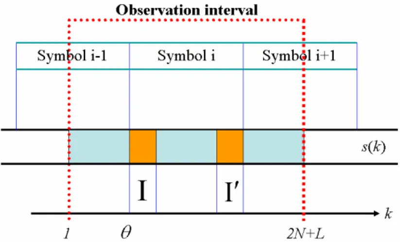
(47) Chapter 3. Frame Synchronization Techniques. Consequently, the guard interval used to estimate the frame location is interfered by the previous symbol.. A synchronizer cannot distinguish between phase shifts introduced by the channel and those introduced by symbol time delays. Time error requirements may range from the order of one sample (wireless applications, where the channel phase is tracked and corrected by the channel equalizer) to a fraction of a sample (in, e.g., high bit-rate xDSL, where the channel is static and essentially estimated only during startup). The effect of a frequency offset is a loss of orthogonality between the tones. The resulting ICI has been investigated in [21].. In the following sections, we assume that the channel is non-dispersive and that the transmitted signal is only affected by AWGN.. We will evaluate our techniques. for both the AWGN channel and a time-dispersive channel by computer simulation in Chapter 5.. 3.2 Correlation Frame Synchronization Techniques 3.2.1 ML Estimation Based on Received Signal [9]. Figure 3.2 Structure of OFDM signal with CP symbols s(k).. 31.

(48) Chapter 3. Frame Synchronization Techniques. Assume that we observe 2N+L consecutive samples of r(k), as shown in Figure 3.2, and that these samples contain one complete (N+L)-sample OFDM symbol.. The. position of this symbol within the observed block of samples, however, is unknown because the channel delay θ is unknown to the receiver. Define the index sets Ι @ {θ ,L , θ + L − 1}. and. Ι′ @ {θ + N ,L , θ + N + L − 1}. (see Figure 3.2). The set Ι′ thus contains the indices of the data samples that are copied into the CP, and the set Ι contains the indices of this CP.. Collect the. observed samples in the (2 N + L) × 1 -vector rˆ @ [r (1)L r (2 N + L)]T . Notice that the samples in the CP and their copies r (k ), k ∈ Ι U Ι ' are pairwise correlated, i.e.,. σ s2 + σ n2  ∀k ∈ Ι : E{r ( k )r ∗ (k + m)} = σ s2 e − j 2πε 0  where σ s2 = E{ s( k ) } and σ n2 = E{ n(k ) } . 2. 2. m=0 m=N. (3.2). otherwise The remaining samples r (k ), k ∉ Ι U Ι '. are mutually uncorrelated. The log-likelihood function for θ and ε , Λ (θ , ε ) is the logarithm of the probability density function (pdf) of the 2N+L observed samples in rˆ given the arrival time θ and the carrier frequency offset ε .. In the following, we will drop. all additive and positive multiplicative constants that show up in the expression of the log-likelihood function since they do not affect the maximizing argument. Moreover, we drop the conditioning on for notational clarity.. Using the correlation properties. of the observations rˆ, the log-likelihood function can be written as. Λ (θ ,ε ) = log f (rˆ θ ,ε )   = log  ∏ f (r (k ), r (k + N )) ∏ f (r (k ))  k∉I ∪ I ′  k∈I    f (r (k ), r (k + N )) f (r (k ))  = log  ∏ ∏  k∈I f (r (k )) f (r (k + N )) k . (3.3). where f (g) denotes the pdf of the variables in its argument. Notice that it is used 32.

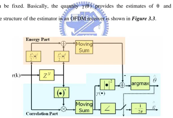
(49) Chapter 3. Frame Synchronization Techniques. The second product Πf(r(k)) in (3.3) is. for both 1-D and 2-D distributions.. k. independent of θ (since the product is over all k) and ε (since the density f (r (k )) is rotationally invariant). Since the ML estimation of θ and ε is the argument maximizing Λ (θ ,ε ) , we may omit this factor.. Under the assumption that rˆ is a. jointly Gaussian vector, (3.3) is shown in the Appendix A to be. Λ (θ , ε ) = γ (θ ) cos(2πε + ∠γ (θ )) − ρΦ (θ ). (3.4). where ∠ denotes the argument of a complex number. γ (θ ) @. θ. ∑. (3.5). 1 θ 2 2 r (k ) + r ( k + N ) ∑ 2 k =θ − ( L −1). (3.6). k =θ − ( L −1). Φ(θ ) =. and ρ =. r ( k )r * (k + N ),. E {r ( k )r * (k + N )}. {. E r (k ). 2. } E { r (k + N ) } 2. =. σ s2 SNR = 2 2 σ s + σ n SNR + 1. (3.7). is the magnitude of the correlation coefficient between r(k) and r(k+N), the asterisk ∗ indicates the conjugate of a complex value and SNR = σ s2 σ n2 .. The first term in. (3.4) is the weighted magnitude of γ (θ ) , which is a sum of L consecutive correlations between pairs of samples spaced samples apart.. The weighting factor depends on the. frequency offset. The term Φ(θ ) is an energy term, independent of the frequency offset ε . ρ ).. Notice that its contribution depends on the SNR (by the weighting-factor. The maximization of the log-likelihood function can be performed in two steps:. max Λ (θ , ε ) = max max Λ (θ , ε ) = max Λ (θ , εˆML (θ )). (θ ,ε ). θ. ε. θ. (3.8). The maximum with respect to the frequency offset ε is obtained when the cosine term in (3.4) equals one. εˆML (θ ) = −. This yields the ML estimation of ε. 1 ∠γ (θ ) + n 2π. where n is an integer. maxima are found.. (3.9). Notice that by the periodicity of the cosine function, several We assume that an acquisition, or rough estimate, of the 33.

(50) Chapter 3. Frame Synchronization Techniques. frequency offset has been performed and that ε < 1 2 ; thus, n = 0 .. Since. cos(2πεˆML (θ ) + ∠γ (θ )) = 1 , the log-likelihood function of θ (which is the compressed log-likelihood function with respect to ε ) becomes. Λ (θ , εˆML (θ )) = γ (θ ) − ρΦ (θ ). (3.10). and the joint ML estimator of θ and ε given r(k) becomes θˆML = arg max{ γ (θ ) − ρΦ (θ )}. (3.11). θ. ε ML = −. 1 ∠γ (θˆML ). 2π. (3.12). Notice that only two quantities affect the log-likelihood function (and thus the performance of the estimator): the number of the CP samples L and the correlation coefficient ρ given by the SNR.. The former is known at the receiver, and the latter. can be fixed. Basically, the quantity γ (θ ) provides the estimates of θ and ε . The structure of the estimator in an OFDM receiver is shown in Figure 3.3.. Figure 3.3 Structure of the ML estimator.. 3.2.2 Peak-Picking Algorithm [9] The peak-picking (PP) algorithm we introduce in this subsection is based on ML estimation describe in 3.2.1.. We can see from (3.10), the first term (correlation part). 34.

(51) Chapter 3. Frame Synchronization Techniques. γ (θ ) dominates the log-likelihood function because the second term (energy part) is almost the same for different θ , then we can reformulate the ML estimator by a correlation function G(n), which is given by L -1. G (n) = ∑ r (n - k ) r * (n - k - N ).. (3.13). k =0. The correlation function G(n) is used for both frequency synchronization and frame timing synchronization.. It represents the correlation of two sequences of L samples. length, separated by N samples, in the received sample sequences as shown in Figure 3.4. The maximum magnitude sample of G(n) is expected to coincide with the first sample of the current OFDM symbol. At this position, samples of CP and their copies in the current OFDM symbol are perfectly aligned in the summation window. Therefore, the estimation θˆm of the frame timing for the mth OFDM symbol can be given as θˆm = arg max Gm (θ ). (3.14). θ ∈Θ. The maximum value of the correlation function is found over a window of Θ = {θ |1 ≤ θ ≤ N + L} for each OFDM symbol (window boundaries are not normally. aligned with that of OFDM symbols) in the receiver.. The estimation frequency error. εˆm is estimated using the phase of the correlation function at θ = θˆm , εˆm = −. 1 ∠Gm (θˆm ). 2π. (3.15). Figure 3.4 Computation of correlation function G(n) using an L-length shift register. 35.

(52) Chapter 3. Frame Synchronization Techniques. 3.2.3 Averaging and Peak-Picking Algorithm [11][15] As suggested in [9], the accuracy of PP algorithm described in 3.2.2 can be improved by averaging Gm (θ ) over several OFDM symbols. Gav (θ ) =. 1 M. M. ∑G m =1. m. (θ ) ,. for θ ∈ Θ. (3.16). where Gav (θ ) is the correlation function averaged over M windows, each of size L+N, and Gm (θ ) is the correlation function evaluated for the mth window. The choice of M, the number of windows (symbols) to average over, in averaging and peak-picking (APP) algorithm mainly depends on the following two factors, (i) Time interval (number of OFDM symbols) over which the arrival time θ and frequency offset ε can be considered to be constant, (ii) Restriction on computational complexity. The above factor (i) is tightly constrained in time fading channels because of the time variant channel delay θ and frequency offset ε . However, in a non-time fading channel (still with multipath and frequency selective fading), this constraint can be significantly relaxed, and θ and ε can be assumed to be constant over significantly long periods.. Although this scenario allows large M values for averaging, the. computational complexity becomes a major problem. We will introduce several low complexity solutions to this problem in the following sections.. 3.3 Low-Complex Frame Synchronization Techniques 3.3.1 Complex-Quantization Algorithm [12] In complex-quantization (CQ) algorithm, we quantize the in-phase and quadrature components of r(k) to form the complex sequence c(k)=Q[r(k)],. 36.

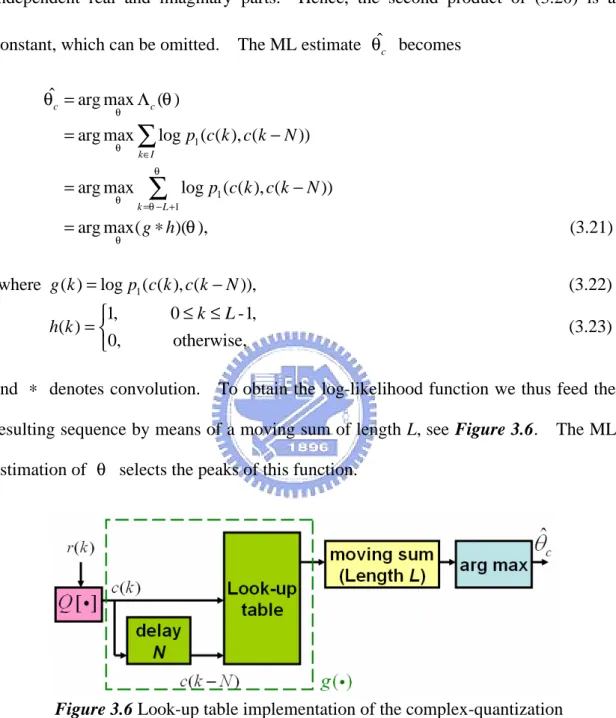
(53) Chapter 3. Frame Synchronization Techniques. k = 1,K , 2 N + L where Q[ g ] denotes the complex quantizer. Q[ x] @ sign(Re{x}) + j sign(Im{x}), +1, x ≥ 0, sign( x) @  −1, x ≥ 0.. (3.17) (3.18). The signal c(k) is a complex bitstream, i.e., c(k) can only take one of the four different values in the alphabet ? = {a0 , a1, a2 , a3}, {1 + j , −1 + j , −1 − j ,1 − j},. (3.19). see Figure 3.5. The sequence c(k) can thus be represented by 2 bits, one for its real and one for its imaginary part.. In spite of this quantization, c(k) still contains. information about θ . A sample c(k), k ∈ Ι , is correlated with c(k + N ) , while all samples c(k), k ∉ Ι U Ι ' , are independent.. Figure 3.5 Geometric representation of the signal set A, and the quadrants Qi , i = 0,1, 2,3 of the complex plane. The probability of all 2N+L samples of c(k) to be observed simultaneously, given a certain value of θ , can be separated in the marginal probabilities for its sample to be observed, except for those samples c(k), k ∈ Ι U Ι ' , which are pairwise correlated. Denote the joint pdf for c(k) and c(k − N ) , k ∈ Ι , by p1( g ), and the pdf for c(k),. k ∉ Ι U Ι ' , by p2( g ). Then, the log-likelihood function of θ given c(k) becomes   Λ c (θ ) = log pθ (c) = log ∏ p1 (c(k ), c(k − N ))g ∏ p2 (c(k ))  . k∉I ∪ I ′  k∈I . 37. (3.20).

(54) Chapter 3. Frame Synchronization Techniques. The ML estimator of θ given c(k), θˆc , maximizes this function with respect to θ . For k ∉ Ι U Ι ' , p2 (c(k )) = 1 4 , since r(k) is zero-mean Gaussian process with independent real and imaginary parts. Hence, the second product of (3.20) is a constant, which can be omitted.. The ML estimate θˆc becomes. θˆc = arg max Λ c (θ ) θ. = arg max ∑ log p1 (c(k ), c(k − N )) θ. = arg max θ. k∈I. θ. ∑. k =θ − L +1. log p1 (c(k ), c(k − N )). = arg max( g ∗ h)(θ ),. (3.21). θ. where g (k ) = log p1 (c(k ), c(k − N )), 1, h( k ) =  0,. (3.22). 0 ≤ k ≤ L -1,. (3.23). otherwise,. and ∗ denotes convolution.. To obtain the log-likelihood function we thus feed the. resulting sequence by means of a moving sum of length L, see Figure 3.6.. The ML. estimation of θ selects the peaks of this function.. Figure 3.6 Look-up table implementation of the complex-quantization ML estimator. In the Appendix B, the complex-quantization ML estimator based on c(k) is determined by calculating the p1( g ). Moreover, it is shown that taking the real part of the correlation between c(k) and c(k − N ) , instead of applying the non-linearity g(k) yields an equivalent and attractive structure for the ML estimator, as illustrated in. 38.