國 立 交 通 大 學
多 媒 體 工 程 研 究 所
碩 士 論 文
應用元球和三维表面重構的冰融化模擬
以及在圖形處理器上之加速
Ice Melting Simulation using Metaballs and
Marching Cubes on GPUs
研 究 生 :李幸宇
指導教授 :黃世強 教授
應用元球和三维表面重構的冰融化模擬以及在圖形處理器上之加速
Ice Melting Simulation using Metaballs and Marching Cubes on GPUs
研 究 生 :李幸宇
Student :Shing-Yeu Lii
指 導 教 授 :黃世強
Advisor :Sai-Keung Wong
國 立 交 通 大 學
多 媒 體 工 程 研 究 所
碩 士 論 文
A Thesis
Submitted to Institute of Multimedia Engineering College of Computer Science
National Chiao Tung University in partial Fulfillment of the Requirements
for the Degree of Master
in
Computer Science October 2012
Hsinchu, Taiwan, Republic of China
應用元球和三维表面重構的冰融化模擬
以及在圖形處理器上之加速
研究生:李幸宇
指導教授:黃世強 教授
國 立 交 通 大 學
多 媒 體 工 程 研 究 所
摘要
在本篇論文中,我們提出了一個新的冰融化模擬方法。這個方法是以粒子為 基礎的模型進行融化模擬。我們將場景中的粒子分為兩種:冰粒子與水粒子。冰 粒子用來表示場景中的冰,而水粒子用來表示水。 在我們的方法中,冰粒子含有一特別屬性,用來存取冰粒子附近水的體積, 我們稱之為虛擬水體積。冰粒子在吸收熱能後會將融化的部分轉化為虛擬水體 積,我們運用在冰模型表面傳遞虛擬水體積的方式模擬融化產生的水以及其在冰 表面的流動。當冰粒子中的虛擬水體積超過預設體積時,則會產生水粒子。 針對冰模型的融化內縮,我們使用新的方法計算標量場中各頂點的標量值, 這個方法將冰粒子的潛熱及虛擬水體積作為標量值計算的參數。接著我們應用三 維表面重構的方法建立冰模型的多邊形網格。 在渲染場景的部分,我們在場景中同時對冰粒子所生成的多邊形網格及水粒 子所代表的元球進行光線追蹤。我們將網格及元球分別使用階層包圍盒建構出階 層式架構,以利於射線的碰撞測試。我們的方法實作於圖形處理器上,在效能上 有不錯的表現。Ice Melting Simulation using Metaballs and
Marching Cubes on GPUs
Student: Shing-Yeu Lii
Advisor: Sai-Keung Wong
National Chiao Tung University
Institute of Multimedia Engineering
Abstract
In this thesis, we propose a novel ice melting simulation method based on a particle-based model. We have two types of particles: ice particles and water particles. The ice particles represent the ice model and the water particles represent water.
In our method, ice particles have an attribute named virtual water volume, which is used to represent the fluid volume around this ice particle. An ice particle may increase its amount of virtual water volume when the latent heat of the ice particle increases. We simulate fluid flowing on the surface of the ice model by transferring the virtual water volume between ice particles. A water particle is produced if the virtual water volume in an ice particle is larger than default volume of the water particle.
For smoothly shrinking ice model, we propose a new method to calculate the potential field. The latent heat of ice particles and virtual water volume are taken into account for computing the potential field. We use marching cubes to construct the polygonal mesh for the ice model.
To render the ice model and water particles, we propose a ray tracing method to render them. The ice model is represented by the polygonal mesh, and water particles are con-structed into metaballs. We use the bounding volume hierarchy (BVH) to create hierarchy constructions to accelerate the process of ray tracing. Our method has been implemented on GPUs. Experiment results show that our method is efficient and compute realistic ice melting simulation.
Acknowledgements
This thesis would not have been possible without the assistance of many people that I gratefully acknowledge.
First, I would like to thank my advisor, Dr. Sai-Keung Wong for his leading in the past two years. He always taught me how to do a good research patiently and gave me many suggestions that helped me a lot to complete this thesis. His suggestion is very helpful for me to obtain the idea and develop the framework of the thesis. I would also like to thank my thesis committee members, Dr. Hung-Kuo Chu, Dr. Wen-Chieh Lin and Dr. Yu-Shuen Wang who evaluated my thesis.
Then, I would like to thank all the labmates for their technical support and spiritual encouragement. They are so friendly so that I can have a pleasant learning environment. It is an honor for me to have such great labmates. Also, I thank my parents and my friends for their unconditional support and patient.
Lastly, I offer my regards and blessings to all of those who supported me in any respect during the completion of the thesis.
Shing-Yeu Lii October 2012
Contents
摘要 i
Abstract ii
Acknowledgements iii
Table of Contents iv
List of Figures vii
List of Tables x 1 Introduction 2 1.1 Motivation . . . 3 1.2 Overview . . . 3 1.3 Contributions . . . 5 1.4 Organization . . . 6 2 Related Work 7 2.1 Melting Simulation . . . 7 2.2 Ray Tracing . . . 8
3 Ice Melting Simulation 10 3.1 Model Voxelization . . . 11
3.2.1 Heat transfer between particles . . . 13
3.2.2 Heat transfer between ice particle and air . . . 14
3.2.3 Thermal radiation from heat source . . . 14
3.3 Phase Transition . . . 16
3.4 Virtual Water Volume Transfer . . . 17
3.4.1 Virtual water volume transfer . . . 17
3.4.2 Water particles creation . . . 19
3.4.3 Special cases handling . . . 19
3.5 Motion of Particles . . . 20
3.6 Marching Cubes Construction . . . 22
4 Rendering 24 4.1 LBVH Construction . . . 25
4.1.1 Morton code construction . . . 25
4.1.2 Morton code sorting . . . 26
4.1.3 Array of split list construction . . . 26
4.1.4 List pairs construction using split list . . . 27
4.1.5 BVH tree construction . . . 27
4.2 Find Isosurface for Metaballs . . . 28
4.2.1 Field function of metaballs . . . 28
4.2.2 Framework for rendering metaballs . . . 29
4.2.3 Bézier clipping . . . 30
4.2.4 The de Casteljau's algorithm . . . 31
4.2.5 Jarvis march algorithm . . . 32
4.2.6 Algorithm . . . 33
4.3 GPU-based Ray Tracing With Meshes and Metaballs . . . 34
5 Experiments and Discussions 38 5.1 Benchmarks . . . 39
5.3 Experiment 2 . . . 44
5.4 Experiment 3 . . . 46
5.5 Experiment 4 . . . 46
5.6 Experiment 5 . . . 48
5.7 More Examples . . . 48
6 Conclusion and Future Works 50 6.1 Conclusion . . . 50
6.2 Future Work . . . 51
List of Figures
1.1 Flow chart for our method. . . 5
3.1 Overview of our ice melting method. . . 11
3.2 (a): Split the scene into voxels. (b): A layer of voxels. . . 12
3.3 A sketch of heat transfer simulation. . . 13
3.4 Two kinds of heat source. The left is a rectangle, and the right is a sphere. 15 3.5 Four cases of water volume transfer. P0is the ice particle we are considering. 18 3.6 Interfacial tension proposes between ice particle and water particle, and between water particles. . . 20
3.7 A sketch of Cartesian distance calculation. . . 21
4.1 The scene is split by the first four bits of Morton code in 2-D space. The red (blue) bits are retrieved from the representative point value of x-axis (y-axis). . . 26
4.2 We assume the Morton codes of triangles A, B, C, and D which have been known. The left hand side shows the calculating process, and right hand side is the result of BVH tree. . . 27
4.3 A sketch of the field function fi. . . 28
4.4 A sketch for rendering metaballs. . . 30
4.5 A Bézier curve with five control points. (a) is the Bézier curve before clipping, and (b) is the curve after clipping. . . 30
4.7 Example of Jarvis March algorithm. The blue line is L0, black lines are
the necessary lines, gray lines and red line are Li, and red line is the line
with the biggest angle calculated with counterclockwise. . . 33
4.8 Flow chart of metaballs rendering. . . 34
4.9 Sketch of ray tracing. . . 35
4.10 Flow chart of ray tracing. . . 36
4.11 The special case occurs when the intersection Hmt is closer to the view target, but the intersection of isosurface is farer than Hmesh. . . 37
5.1 A series of snapshots for Cube. . . 39
5.2 A series of snapshots for Sphere. . . 40
5.3 A series of snapshots for Bunny. . . 40
5.4 A series of snapshots for Dragon. . . 40
5.5 Execution time of each step of ice melting simulation relates to the number of water particles. The benchmark used here is Cube. . . 42
5.6 Execution time of ice melting simulation with different level of voxeliza-tion. The benchmark used here is Sphere. . . 44
5.7 This is a snapshot of the Bunny ear. In the same frame, the left hand side is the method without using metaballs, and the right hand side is our method. The red and yellow circles are different parts between two pictures. . . 45
5.8 This is also a snapshot of the Bunny ear. The red and yellow circles are different parts between two pictures. . . 45
5.9 The snapshots of real melting ice cube. www.youtube.com/watch? v=WgjksZoznuA 46 5.10 The top three pictures are the ice melting results proposed in [IUDN10], and the bottom three pictures are our results. . . 47
5.11 The top three pictures are the rendering results for the heat source Sphere, and the below three pictures are the rendering results for the heat source Rectengle. . . 48
5.12 A bunny on the table. . . 49
5.14 Icicles in the cave. . . 49 6.1 The sketch map of problem in meshes shrinking. . . 52
List of Tables
5.1 Model complexities and number of ice particles. The columns of table from left to right are number of triangles for input benchmark, number of vertices for input benchmark, number of ice particles, and number of grids
of marching cubes (MC). . . 41
5.2 The experimental results of ice melting simulation. The first two columns are average number of water particles and number of triangles constructed by marching cubes. The right part is the average execution time for each step. (msec) . . . 41
5.3 Breakdown of virtual water volume transfer. (usec) . . . 41
5.4 Breakdown of motion of particles. (msec) . . . 42
5.5 Execution time of rendering. (msec) . . . 43
5.6 Model complexity and timing comparisons (in msec) of marching cubes construction and rendering with and without metaballs. The model we use is Bunny. . . 44
5.7 Execution time of our ray tracing method with CPU-based BVH construc-tion, with GPU-based BVH construcconstruc-tion, and without BVH construction for metaballs. The model we use is Dragon. (msec) . . . 47
Chapter 1
Introduction
Simulation of natural phenomena, such as water, fire, and cloud, has been widely used for applications, including commercial movies, games, and advertisment. Ice appears in everyday life, for examples, ice cubes in drinks, frozen lakes, and icicle cave, etc. In movies and games, ice melting is often depicted. Therefore, the focus of this thesis is on achieving both realistic and high performance for ice melting simulation.
However, ice melting is a challenging research topic because of the complex char-acteristics of ice. First, ice is semitransparent. Light can go through ice and it is also reflected by ice. Second, when a portion of ice begins to melt, it becomes water directly. There is no semi-solid produced in the ice melting process, and the solid part will shrink. Third, water moves on the surface of ice. Nowadays, there are many techniques that have been proposed for ice melting. We want to find a way to combine these studies, and also render the result as realistically as possible. It is a big challenge.
In this thesis, we propose a novel method for ice melting simulation based on a particle-based model. There are two types of particles: ice particles and water particles. The ice particles represent the ice model, and the water particles represent water which is melted from the ice model. The ice particle has an attribute named virtual water volume. It is used to represent the water volume around the ice particle. We propose a method to transfer the virtual water volume between ice particles and produce water particles.
for the ice model. The latent heat of ice particles and virtual water volume are taken into account for computing the potential field. We use marching cubes to construct the polygonal mesh for the ice model.
To rendering ice and water together, we propose a ray tracing method to render them at the same time. The ray tracing method can render the scene with transparent objects. Furthermore, we implement our system on GPUs and apply the OpenCL libraries for the parallel computation.
1.1
Motivation
Ice is common in everyday life, and it is often seen on games and movies. In addition, ice melting is one of the important natural phenomena in the real world. It is also an important research area of physical simulation.
However, it is difficult to simulate ice melting realistically because the shape of the solid part in simulating is not easily handled. Also, the shape of water droplet is difficult to be constructed precisely based on the meshes, such as using marching cubes, in a relatively low resolusion. It takes a lot of time to render ice and water as they are a transparent object. We want to utilize the methods combined with marching cubes and metaballs to sim-ulate the process of ice melting. Our method can model the ice model which shrinks continuously while the ice model melts. Our method also handles water droplets merging.
1.2
Overview
Our method has two components: ice melting simulation and rendering.
The ice melting simulation is based on a particle-based model. The thermal energy transferring within the object is considered. A set of ice particles represent ice, and these ice particles transfer heat between each other. The latent heat will be saved in each ice particle and the ice particle disappears when it obtains enough heat of fusion. From an-other perspective, relative proportion of volume of an ice particle to the latent heat should
becomes water. An attribute named virtual water volume is associated with an ice particle. It represents the water volume nearby the ice particle. We simulate the water flows on the surface of ice model by transferring virtual water volume. Furthermore, water particles are constructed if the amount of virtual water volume in an ice particle is too much. The smoothed particle hydrodynamics (SPH) is used to simulate the motion of water in our method. It calculates the force for water particles based on the properties of water with regard to pressure, viscosity, and density.
We construct a polygonal model for ice particles using the marching cubes method, while water particles are represented by metaballs. The latent heat of ice particles and the ratio of water volume are considered as for computing the potential field. The field value is affected by the latent heat and the ratio between water volume and ice particles. With the increase in the latent heat of an ice particle, the relative proportional volume of the ice particle change to water, and then the field value decreases. On the other hand, the field value increases if the water volume becomes larger.
To render ice model and water particles together, we use the ray tracing method. We separate the ice particles and water particles, and render them using different methods. We use the marching cubes to construct the polygonal mesh for the ice model, Then, we build a BVH construction for them. Water particles are represented by metaballs. We use an approximate algorithm to find the isosurface for the metaballs. Each ray is tested for intersection for meshes and metaballs.
Figure 1.1 is the process for our method. The seven steps are shown below:
1. We input a polygonal model and voxelize it. Each voxel represents an ice particle. 2. We compute heat transfer for all particles. There are three ways that an ice particle
can absorb heat: other particles, air, and heat source. An ice particle is removed if the latent heat of the ice particle is higher than the required heat energy.
3. The relative proportion of the volume of an ice particle to the latent heat becomes virtual water volume and transforms between ice particles from high to low. A new water particle is constructed if the virtual water volume in an ice particle is too much.
Figure 1.1: Flow chart for our method.
4. Water particles move according to some forces, including hydromechanics, gravity, and interfacial tension, etc.
5. We use a new method to compute the potential field. Then, we construct meshes for ice particles using the marching cubes method.
6. We create BVH for the meshes and metaballs.
7. The ray tracing method traces on the BVHs of the meshes and metaballs, and shows the rendering result on the screen. Then, we go back to step two for the next frame.
1.3
Contributions
The major contributions of this thesis are described as follows.
1. We propose a novel ice melting simulation method based on a particle-based model. We use the virtual water volume transfer method to simulate water flowing on the surface of the ice model. Virtual water volume is transferred between ice particles. The virtual water volume tends to transfer from ice particle of higher position to ice
particle of lower position. A water particle is constructed when the virtual water volume in an ice particle is larger than a default volume.
2. We propose a new method to calculate the potential field. The latent heat of ice particles and virtual water volume are considered for computing the potential field. The latent heat of the ice particle increasing causes the field value around the ice particle to decrease. In contrary, the field value increases if the virtual water volume increases around the ice particle. We use marching cubes to construct a polygonal mesh for the ice model. In this way, we can model the model shrinks when the ice model melts.
3. To render ice model and water particles, we propose a new method for ray tracing to the mesh and metaballs in the same scene. We use bounding volume hierarchy (BVH) to create hierarchies for these two parts (i.e., meshes and metaballs). A special principles of judgment is proposed to find intersections for rays using ray tracing method.
4. The main parts of our system is implemented on GPUs. We use OpenCL to perform the parallel computation.
1.4
Organization
The remaining chapters of the thesis are organized as follows. Chapter 2 reports the related work about melting simulation and ray tracing. We present our ice melting simu-lation method in Chapter 3. Our rendering algorithm is illustrated in Chapter 4. Chapter 5 presents experiments and discussions. Finally, Chapter 6 presents the conclusion and future works.
Chapter 2
Related Work
There are two main components in our system: melting simulation and ray tracing method. For the melting simulation, we use a particle-based heat transfer method. For rendering, GPU-based ray tracing is proposed in our system. In the following sections, we present the related work for the melting simulation and ray tracing method.
2.1
Melting Simulation
There are many researches relate to melting solid object in the past. The basis of the concept utilizes the thermodynamic heat transfer to conduct heat, and melts object.
Fujishiro et al. [FA01] simulated the melting of ice by using the morphology. This method voxelize the polygonal model and conduct heat between voxels. However, this method neglects fluid part that is formed due to melting.
Carlson et al. [NN94] melted solid object such as wax or clay, and also handled melted fluid by using Navier-Stokes equation. Although this method can simulate melted fluid for the soil-like high stickiness object, it does not conform to the properties of water.
There were many techniques on melting ice [FGFR06][FM07][CMJG07]. These methods also handle the motion of water, but they take several minutes for each frame.
Zhao et al. [ZY06] employed GPUs to accelerate the process. Solenthaler et al. [SSP07] developed a unified particle model to simulate solid-fluid interactions, including
melting, solidification, merging and splitting. Although the method can simulate melting object at an interactive frame rates, it doesn't consider to the motion of water droplet.
Iwasaki et al. [IUDN10] proposed a method implemented on GPUs. The method handles ice, water, and water droplet when melting occurred, and the execution time is also less than the previous approaches. Our method is developed based on their method.
2.2
Ray Tracing
Ray tracing is one of the rendering technologies that is the most commonly used. The property of ray tracing is that ray tracing can produce realistic scene according to lights and objects characteristics, such as material and transparently. The first algorithm is proposed by Arthur Appel et al. [App68] in 1968, but they didn't consider to the light of reflection. Turner Whitted et al. [Whi80] proposed a method which used recursive ray tracing including the effects of reflection, refraction and shadow. This method can render realistic scene.
In the past, ray tracing cannot be used on the real-time or interactive system because of a large amount of calculation. Ray tracing can only use to construct off-line videos such as movies or animations. With the era of progress, two important techniques accelerate the process of ray tracing.
In order to speed up ray tracing performance, previous techniques bundle many rays in a packet, and use multithreading or SIMD to traverse and test intersection for rays. This method successfully improves overall performance. The algorithm proposed by Wald et al. [WMG+07] enlarges the packet size from 2*2 to 32*32, and greatly reduces the number
of intersection test.
Due to the development of Graphic Processing Unit (GPU), GPU became the main tool for parallel computing. Ray Engine [CHH02] was the first ray tracing system imple-mented on GPUs. Later, more and more techniques utilized multiprocessors of GPUs to improve performance. For instance, Purcell et al. [PBMH02] employed programmable graphics hardware to implement ray tracing algorithms.
NVIDIA developed Compute Unified Device Architecture (CUDA) [NVI] language in 2008. This is a parallel computing architecture for graphics processing. Further, Open Computing Language (OpenCL) [Khr09] was developed by Apple Inc. in 2009, which is a framework for writing programs that execute across heterogeneous platforms consisting of central processing unit (CPUs), graphics processing unit (GPUs), and other processors. Since the development of these two tools, researchers can design the program with parallel computing on GPUs effectively.
Ray-triangles intersection test spends the most time in ray tracing algorithms. There-fore, a lot of acceleration constructions are proposed, such as kd-tree or Bounding Volume Hierarchy (BVH). Most of the kd-tree constructions [FS05][HSHH07][PGSS07][ZHWG08] and BVH constructions [WMG+07][LGS+09][PL10] were implemented on GPUs. We use the method proposed by Lauterbach et al. [LGS+09] to create the acceleration
con-structions for our meshes.
In our system, we use an algorithm proposed by Kanamori et al. [KSN08] to render water particles. This method improves realistic for the water droplets, but the execution time increases when the number of water particles is higher. Kanamori et al. [GPP+10]
Chapter 3
Ice Melting Simulation
Ice is not a viscous substance, and water will flow when ice becomes water from solid-state. There is no semi-solid in the ice melting process. The water from melted ice will move on the surface of the ice model. Thus, the ice melting simulation has been widely studied.
We propose a novel ice melting simulation method based on a particle-based model. There are two types of particles: ice particles and water particles. The ice particles rep-resent the ice model. Each ice particle has some attributes, such as position, temperature, and latent heat, etc. There is an attribute named virtual water volume for an ice particle, which is used to record the water volume produced by melting a portion of the ice particle. The water particle also has some attributes, such as position, velocity, and force, etc.
Basically, the system of ice melting simulation has two components: heat transfer and shape reducing. We use the method proposed by Iwasaki et al. [IUDN10] to transfer heat. The amount of latent heat of an ice particle will be computed using the equation of thermal energy transfer, and ice model will be melted via increasing latent heat. We calculate virtual water volume transfer and employ marching cubes method to shrink the shape of the ice model smoothly.
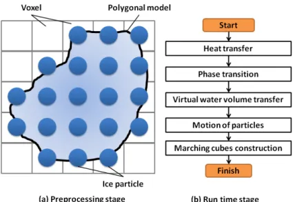
The flow chart of our ice melting method is shown in Figure 3.1. In the preprocessing stage, we load a polygonal model and voxelize the model to a set of 3-dimension voxels. Each voxel in the set represents an ice particle.
Figure 3.1: Overview of our ice melting method.
In the run time stage, we do several steps each time step, including heat transfer, phase transition, virtual water volume transfer, motion of particles, and marching cubes construction. We introduce each step in the following sections.
3.1
Model Voxelization
Our method is based on particles, and motions of water particles are calculated based on smoothed particle hydrodynamics (SPH). Therefore, we need to transform the inputted polygonal models into particles.
Voxel is short for "volume pixel", and it is a cube in a 3-D lattice. In simple terms, we can partition the 3-D scene into many voxels, and use the voxel model to represent the polygonal model. To achieve model voxelization, we extend the 2-D scan-conversion algorithm to 3-D space using [Kau87]. By using the scan-conversion algorithm, the voxels which belonged to the meshes of the model will be found and collected in a set ν. Next, we introduce this method in detail.
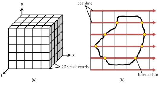
We partition the 3-D scene into uniform voxels. These voxels will be divided into several 2-D layers by using one of the three axes, as shown in Figure 3.2(a). In each 2-D layer, we shoot rays along the direction of rows and find intersections between the rays
Figure 3.2: (a): Split the scene into voxels. (b): A layer of voxels.
and polygonal model, as shown in Figure 3.2(b). In general, each ray will intersect the model in an even amount of times if the starting position of the ray is outside the polygonal model. The intersections are the shells representing the surface of the polygonal model. Then, we scan each row again and collect the voxels which are inside the shell surface to the set ν one to another voxel. We repeat the same process for all 2-D layers. Finally, the voxel model will be constructed by using the voxels that belong to the set ν.
After collecting all the voxels we want, each voxel is designated as an ice particle. Each ice particle has some attributes: temperature, latent heat, position, virtual water vol-ume, and indices of neighboring particles, etc. Temperature and latent heat are utilized in the method of heat transfer and for deciding the phase of particles. Virtual water volume is used for recording the amount of water volume which is produced by melting a portion of the ice particle. We use an attribute called "indices of neighboring particles" to record the six neighboring particles. If the number of neighboring particles is less than six, the ice particle is an outward particle, and its will absorb the heat from the air.
3.2
Heat Transfer
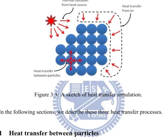
The ice particles absorb thermal energy and melt at each time step. The method is based on Iwasaki et al. [IUDN10]. There are three ways to absorb heat for the ice particles, as shown in Figure 3.3: other particles, air, and the heat source.
Figure 3.3: A sketch of heat transfer simulation.
In the following sections, we describe these three heat transfer processes.
3.2.1
Heat transfer between particles
The particle i absorbs heat from the other particles, which is calculated from the equa-tion: ∂Ti ∂t = Cd ∑ j∈Ni mj(Tj− Ti) ρj ∇2 W (rij, re) (3.1) ∇2 W (rij, re) = 45 Πr6 e (re− rij) (3.2)
where ∂t is the time step. Ti is the temperature of the particle i, Ni is a set of particles
whose distance rijfrom particle i are smaller than the effective radius re, W is a smoothing
kernel function as the equation used for calculating viscosity, as shown in Equation 3.2, and Cd is the thermal diffusion constant changing from different phase of particle i (i.e.
ice or water). We use Equation 3.1 to calculate heat transfer between particle i and its neighboring particles.
3.2.2
Heat transfer between ice particle and air
In general, we assumed that air is made up of particles, and heat transfer between air and ice particles is calculated via Equation 3.1. However, this method requires extra air particles and will increase the simulation time. In order to achieve better performance, we approximate the temperature of air particles as a constant Tair. Therefore, the heat transfer
between ice particle and air can be simplified into the Newton's law of cooling:
Qi = h(Tair− Ti)δA, (3.3)
where Qiis the amount of heat absorbed by an ice particle i, h is the thermal conductivity,
and δA is the surface area of particle i which contact to the air. To obtain δA, we need to compute the number of neighbors by using the attribute "indices of neighboring particles". By subtracting the number of neighbors from six, we can get the number of face touching the air, and the sum of area for these faces can be accumulated. After we compute Qi, the
increase in the temperature ∆T is calculated from: ∆T = Qi
Cm, (3.4)
where C is the heat capacity of the ice, and m is the mass of an ice particle.
3.2.3
Thermal radiation from heat source
There are some heat sources in the scene, such as the sun or a heater, and these heat sources will radiate thermal energy to the scene. We assume that the heat source emits some particles carrying thermal energy, and we call these particles thermal photons. The total thermal energy E is released from the heat source at each time step, and we can compute the E via the equation:
E = εσTs4Hdt, (3.5) where ε is an emissivity factor, σ is the Stefan-Boltzmann constant, Tsis the temperature
of the heat source, H is the surface area of the heat source, and dt is the time step. The sum of the thermal energy in each thermal photon is E. Therefore, at each time step, a
photon has thermal energy Epcomputed from Ep = E
N, where N represents the number
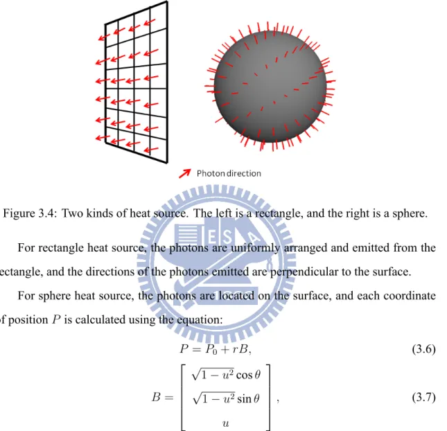
of photons emitted in a time step. Here we assume two kinds of heat source, rectangle and sphere, as shown in Figure 3.4.
Figure 3.4: Two kinds of heat source. The left is a rectangle, and the right is a sphere. For rectangle heat source, the photons are uniformly arranged and emitted from the rectangle, and the directions of the photons emitted are perpendicular to the surface.
For sphere heat source, the photons are located on the surface, and each coordinate of position P is calculated using the equation:
P = P0+ rB, (3.6) B = √ 1− u2cos θ √ 1− u2sin θ u , (3.7)
where P0 is the central position of sphere, r is the radius of the heat source, and B is a
vector related to the spherical coordinates which are based on the angles θ and ϕ. The parameters θ and u = cos ϕ of each photon are uniformly set in the limit interval θ ∈ [0, 2Π), and u∈ [−1, 1]. The ray Dp of the photon emitting from the sphere heat source is computed as Dp = P − P0.
We calculate the number of photons that hit to each ice particle using the ray-voxel intersection test. To speed up the intersection test, our method test an intersection
effi-[AW87]. The increase in thermal energy δQi for the ice particle i is the product of the
multiplication of the thermal energy Epby the number of photons hitting the particles i.
3.3
Phase Transition
We assume that an ice particle is constructed by a lot of molecules. When the tem-perature of ice particle increases to 0◦C, the ice particle begins to absorb enthalpy of
fusion(i.e., heat of fusion for ice). A portion of the ice particle transfer when the latent heat of the particle increases. We construct an attribute in each ice particle, named virtual water volume, to record the water volume produced by melting a portion of the ice parti-cle. The ice particle disappears when the temperature of the ice particle increases to 0◦C,
and also when the ice particle obtains enough latent heat. Our method has two steps in the phase transition process:
1. Accumulate the thermal energy to each particle. The thermal energy will increase the temperature or the latent heat of the ice particle. The ratio of latent heat will affect the increase of the amount of the virtual water volume.
2. Check whether the ice particle absorbs enough thermal energy; if so, it is removed. Renew the attribute "indices of neighboring particles" when the neighbors of ice particle i disappear.
In the heat transfer process which we have described in previous section, each particle obtains heat value δQi. For each ice particle i, we try to increase the temperature up to
0◦C by transforming energy δQito temperature ∆T using Equation 3.4. Further, the rest
of the thermal energy are added into the latent heat Eiwhen the temperature reaches 0◦C.
We use the equation to calculate the ratio of the latent heat Eratio, as shown below: Eratio=
Ei Etotal
, (3.8)
where Etotalis the amount of energy which is needed to melt an ice particle:
Ew is a constant of heat energy related to the type of material, and m is mass of an ice
particle. To melt a kilogram of ice, about 79720 calories heat energy is needed.
We assume that a portion of ice particle transform to water when latent heat increases. We use the following equation to transform a portion of volume of the ice particle into virtual water volume:
∆V = Vd∗ d
dtEratio, (3.10)
where ∆V is the amount of water volume in this time step that we add into virtual water volume of ice particle, and Vd is default volume of whole ice particle. All ice particles
will increase the virtual water volume in each time step based on the ratio of latent heat. The ice particle is removed when the Eiincreases up to enthalpy of fusion Etotal. In
other words, the ice particle disappear when Eratio is equal to 1. When the ice particle i
absorbs enough heat energy it and disappears, we remove i from the attribute "indices of neighboring particles" for the particles which is nearby the particle i.
3.4
Virtual Water Volume Transfer
Virtual water volume will be transferred between neighbors of ice particles from high position to low position. We simulate the water flow on the surface of the ice model using virtual water volume transfer. Furthermore, water particle is produced if there is too much virtual water volume in an ice particle at the same time. The virtual water volume will be a factor for effecting the marching cubes construction.
In the following sections, we will illustrate this method in detail. It will be separated into two steps: virtual water volume transfer, water particles creation. After that, we will describe two special cases in our method, and how we have handled them. The influence for marching cubes from the virtual water volume will be described in Section 3.6.
3.4.1
Virtual water volume transfer
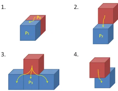
Figure 3.5: Four cases of water volume transfer. P0is the ice particle we are considering.
of the features of water is that it flows downwards, so we use this feature to transfer the virtual water volume between ice particles. There are four cases to transfer the virtual water volume via ice particles from high to low, as shown in Figure 3.5.
For each ice particle, we calculate the virtual water volume transfer for its four sides (excluding upper and lower side). Each surface will be tested for these four cases (Fig-ure 3.5) in a sequence.
In the first case, the ice particle P0 is tested with the neighboring particles. If there
exists an ice particle P1 and P1 has less amount of virtual water volume than P0, we put
P1into the set of wanted particles W . If there is no P1, the virtual water volume can flow
via that surface from high to low, and then we check case two. We put the particle P2into
set W if P2 exists at the position like the case two which is shown in the figure. We will
perform case three if the P2 doesn't exist, because there is no particle blocking the flow.
Case three establishes if there is a particles P3there, otherwise, case four happens.
We check the four cases for four side surfaces and save all the particles which can be flowed through into the set W . Then, we reduce the portion of virtual water volume from P0and allocate the amount of virtual water volume to particles in W based on virtual
water volume of each particle. This is because water tends to transfer and converge at the place with more water.
3.4.2
Water particles creation
Sometimes, the virtual water volume in an ice particle has more than the default vol-ume of a water particle Vdat the same time and there is no other way to transfer it. This ice
particle will decrease for the same amount of Vdand create a water particle. This situation
occurs usually on the bottom of ice model or drooping tip, such as icicles on the roof. We create a water particle at the position nearby the center of this ice particle, and we give an initial velocity to this new water particle. The direction of the initial velocity goes outward to the ice model to avoid the attractiveness of the interior ice particles. These water particles moves based on the smoothed particle hydrodynamics (SPH) and we will describe in Section 3.5.
3.4.3
Special cases handling
There are two special cases in our virtual water volume transfer method. First, when an ice particle absorbs enough amount of heat and is removed, the virtual water volume in this ice particle will be lost. However, this result is not correct because the total volume of the object is different after we ignore the virtual water volume in ice particles which have been removed. To solve this problem, we transfer the virtual water volume from the ice particle to the neighbors of this ice particle.
Second, the water particle may drop onto ice particles and stay on them, leading to obvious unnatural result if the particle size is big. Therefore, we allocate the volume of the water particle into the virtual water volume of these ice particles and delete the water particle which is laid on the ice particles. In other words, this water particle changes back to virtual water volume and flows on the surface of the ice model.
3.5
Motion of Particles
The smoothed particle hydrodynamics (SPH) is used to simulate the motion of water particles. The motion of the particles are calculated based on the Navier-Stokes equations:
du dt =− 1 ρ∇p + µ∇ 2+ f, (3.11) ∇ · u = 0, (3.12) where u is the velocity, ρ is the density, p is the pressure, µ is the dynamic viscosity coef-ficient, and f represents the external forces. For particle-based simulation, the continuity equation shown here as Equation 3.12 can be preserved automatically if no particle is deleted or inserted and the particle mass is constant. The first and second terms on the right-hand side of Equation 3.11 are the pressure force fpress and the viscosity force fvis,
respectively. So, the Equation 3.11 can be changed to:
du
dt = fpress+ fvis+ f, (3.13)
where the third term f in the Equation 3.13 includes gravity, force of collision response, and interfacial tension fi.
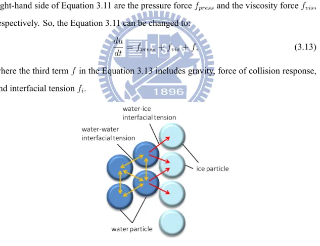
Figure 3.6: Interfacial tension proposes between ice particle and water particle, and be-tween water particles.
The paper [IUDN10] observed the ice melting phenomenon and suggested that wa-ter particle will move on the surface of the ice model before falling down, as shown in
Figure 3.6. To implement this phenomenon, the virtual interfacial tension fiof the water
particle i is calculated by the following formula:
fi = ∑ j∈Nwater i kw xj − xi ∥xj− xi∥2 + ∑ j∈Nice i kice xj − xi ∥xj− xi∥2, (3.14)
where xi is the position of the particle i, kw is the coefficient of the interfacial tension
between the water particles, kiceis for water-ice interfacial tension, and Niwater (Niice) is a
set of water (ice) particles nearby particle i.
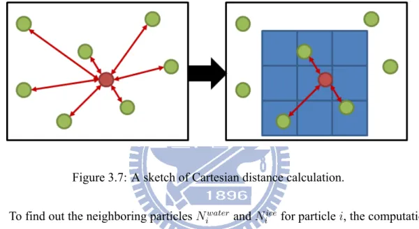
Figure 3.7: A sketch of Cartesian distance calculation. To find out the neighboring particles Nwater
i and Niicefor particle i, the computation
cost is high in calculating the distance two particles. In order to achieve an efficient simu-lation, we calculate the Cartesian distance for two particles before we calculate the actual distance, as shown in Figure 3.7.
The scene is split into many cubes with same size, and the width of one cube is one Cartesian unit. First, each particle is represented by a Cartesian coordinate, which is a 3-D index Cibased on the position of particle via Cartesian unit. Thus, we change the length
of effective radius of particle i to the number of Cartesian unit Nr, and obtain the effective
region for the particle i. The Cartesian distance Nmaxbetween particle i and j is obtained
using this formula:
Nmax = max(|Cix− Cjx|, |Ciy− Cjy|, |Ciz − Cjz|). (3.15)
method can reduce calculating timing by removing some unnecessary distance calculation when two particles are too far away.
3.6
Marching Cubes Construction
There are two features in our marching cubes method, and we describe them as below. First, we only need to construct the marching cubes for the ice particles. Our render-ing method uses the method proposed in [KSN08] to find the isosurface for water particles directly via ray tracing. Therefore, we don't need to construct the marching cubes for the water particles. The advantages are that we can reduce the constructing time of marching cubes construction for these water particles. Also, we get fewer triangles from marching cubes construction, which speed up the ray-triangle intersection test in the rendering pro-cedure. Best of all, the shape of water particles is represented more realistically by using the method proposed in [KSN08] than using marching cubes method.
Secondly, we propose a novel method to calculate the potential field. We observe that the animation of ice meshes is discontinuous when the ice particle immediately dis-appears. That is because the influence from the ice particle to the potential field is lost. However, ice melting simulation should be a continuous animation and the meshes made by marching cubes cannot instantaneously change. The meshes should smoothly contract inward. Moreover, the virtual water volume that retains in each ice particle should be taken into account. Therefore, the field function is modified to:
Φ(x) = (∑ j (E∗ (1 − r h)) 2) 1 2 , (3.16)
where E has two parts:
E = Es+ Ewv. (3.17) Es is computed based on the shrinking ratio:
Es = 1−
3
√
Eratio, (3.18)
where Eratiois defined in Section 3.3. The ice particle is removed when the Eratiobecomes
ice volume V and water will change according to Eratio. Also, the number of melted
molecules is proportional to total amount of volume V of melted molecules, Therefore, we understand that Eratio is a 3-D unit. The field function for marching cubes is based
on distance between the vertices of cubes and the particle. However, the unit for field function is 1-D, while Eratiois a 3-D unit. Therefore, we use the Equation 3.18 to obtain
reasonable value for Es.
The second term of Equation 3.17 Ewv is based on the virtual water volume in ice
particle, shown below:
Ewv= 3
√
Vi Vd
, (3.19)
where Viis the amount of of virtual water volume in the ice particle i, and Vdis the default
water volume of whole ice particle.
We can prove this equation by skipping the virtual water volume transfer step (i.e., the method introduced in Section 3.4). Then, Vi is equal to V , Eratio ≡
Vi Vd
, and E =
Es+ Ewv= 1. We add E into the basic equation of field function. After that, the meshes
Chapter 4
Rendering
To render transparent fluid realistically, we use ray tracing to render the scene. The ray tracing technique can compute the reflection and refraction of light, so it is good for transparent objects. However, ray tracing costs a lot of time on calculating the intersection between rays and objects in the scene, and also takes some time on computing the color for the pixels. Therefore, we implement our system on the GPUs to accelerate computation time. We separate the ice particle and water particle and use a unique methods to test for the intersections.
We transfer the ice particles into polygonal mesh as described in Section 3.6, and the accelerate construction linear bounding volume hierarchy (LBVH) is proposed. There-fore, the computation time for the intersection test is reduced by tracing rays within the hierarchy construction.
For water particles, our method is based on the method proposed by Kanamori et al. [KSN08]. In their method, the isosurface of these water particles (metaballs) can be found using ray tracing with the special principles of judgment. As illustrated in the Section 3.6, the advantages of separating ice and water particles are that we can reduce the construction time for these water particles. We also get fewer triangles from the marching cubes method, which speeds up the testing of ray-triangle intersection when we render the scene. Most of all, the shape of water particles is represented more realistically by using the method proposed in [KSN08] than using the marching cubes method.
In the following sections, we will introduce three components: LBVH construction, the method to find the isosurface for water particles, and GPU-based ray tracing based on meshes and metaballs.
4.1
LBVH Construction
The most time-consuming part of ray tracing is the ray-triangle intersection test. This is especially true for transparent objects, which requires at least three times of test (inci-dent ray, reflection ray, refraction ray). Therefore, many researches focus on hierarchy accelerate construction, such as kd-tree or bounding volume hierarchies (BVH). We select the linear bounding volume hierarchy (LBVH) method, which is proposed by Lauterbach et al. [LGS+09]. This method uses the concept of Morton Code (or Z-Order Curve) to sort triangles, and sorted list to construct BVH parallelly.
In ice melting simulation, the marching cubes method generates different polygo-nal mesh in each frame, so we need to construct a new BVH at each time step. LBVH can quickly build the accelerate construction with GPUs, so it is an essential part for our method. Now, we will describe all the steps of the LBVH construction in detail.
4.1.1
Morton code construction
We calculate the axis-aligned bounding box (AABB) for each triangle and take the barycenter of each primitive AABB as its representative point. We can quantize each of the 3 coordinates of representative points into k-bit binary digits. The 3k-bit Morton code for a point is constructed by interleaving the successive bits of these quantized coordinates. For example, the representative points of a triangle is (0, 1, 3), and we assume k = 2. It is changed to (00, 01, 11) as the binary digits, and then we interleave the successive bits into 100110 via the sequence of axes (z, y, x).
4.1.2
Morton code sorting
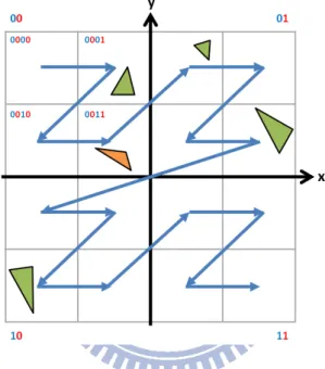
After changing all representative points to Morton code, we sort them using the paral-lel radix sort algorithm which is proposed by NVIDIA [NVI] on GPUs. Morton code has a corresponding relationship with the space. Figure 4.1 shows a 2-D sketch map of this construction. Sorting the representative points in increasing order of their Morton codes will lay out these points in order along a Morton curve (blue arrow in Figure 4.1). Thus, it will also order the corresponding primitives in a spatially coherent way.
Figure 4.1: The scene is split by the first four bits of Morton code in 2-D space. The red (blue) bits are retrieved from the representative point value of x-axis (y-axis).
4.1.3
Array of split list construction
The two triangles have different Morton codes when these two triangles are in the different child space. After sorting the Morton codes, we successively extract two adjacent Morton code in the sorted list and compare them from the highest-bit. Then, we build an array named split list to save the position ℓ of the first different bit into the array. For example, there are two Morton codes, 000111 and 001110 for two different triangles. The first different bit of two Morton codes is the 3rd bit, so ℓ = 3. The data in split list represent the level in the BVH tree where the two triangles are separated.
4.1.4
List pairs construction using split list
We expand the split list array into list pairs S(i, ℓ) as shown below:
S(i, ℓ) = [(i, ℓ), (i, ℓ + 1), ..., (i, 3k)], (4.1) where the first term of (i, ℓ) is the index of the triangle i and the second term is the levels of the splits between the primitives. If we perform this computation for each data item in thesplit list and concatenate all such lists, we get a list of all the splits in the tree sorted by the index of the triangles in the linear Morton order. Once we have this list, we sort it again by level (i.e., the second term of each pair). This tells us how to split the triangle list into various nodes on the BVH construction.
4.1.5
BVH tree construction
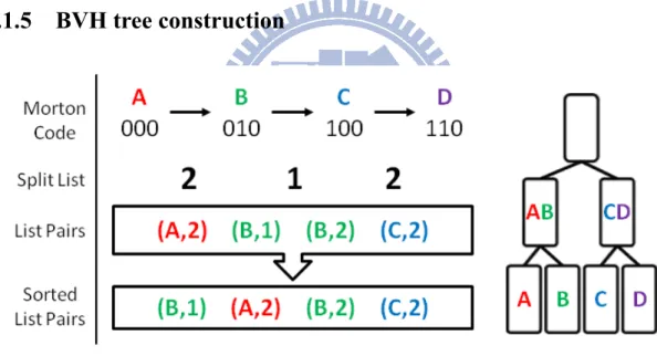
Figure 4.2: We assume the Morton codes of triangles A, B, C, and D which have been known. The left hand side shows the calculating process, and right hand side is the result of BVH tree.
According to the sorted list pairs, we put all the triangles into a tree structure. Fig-ure 4.2 is an example. We assume that the split list computed for the four triangles is 2, 1, and 2, then, the list pairs will be (A,2), (B,1), (B,2), and (C,2). After we sorted the list pairs by the second term, the BVH construction will be set up. The triangles will be partitioned
into two sets AB and CD and we put them in the level 1 nodes in the BVH tree based on the first list pairs (B,1). Furthermore, the triangles are split in four different nodes in level 2 via the next three data of sorted list pairs (A,2), (B,2), and (C,2). Therefore, we finished the BVH construction for the meshes of the ice model using GPUs.
4.2
Find Isosurface for Metaballs
We separate the ice particles and water particles, and use different ways to test inter-section for them. Here we introduce the method used for testing the interinter-section for water particles. The method is based on the method proposed by Kanamori et al. [KSN08], and they use a metaball to represent a water particle.
To render the shape of the metaballs smoothly, the isosurface of these metaballs can be found using ray tracing with the special principles of judgment. Each metaball has a density field, and a set of nearby metaballs represents a smooth surface by the way of combining their density fields. In the following sections, we will introduce the method to find the isosurface for the metaballs.
4.2.1
Field function of metaballs
Figure 4.3: A sketch of the field function fi.
We use the density field function fi to represent the metaball i based on the distance r from the central of metaball Pito the point x, as shown in Figure 4.3. The fi has a finite
support Ri, and Rirepresents the effective radius of metaball i. Thus, fi(r) = 0 if r ≥ Ri.
For N metaballs, the shape of the isosurface is defined by the point x∈ R3 in below:
f (x) = N∑−1
i=0
qifi(∥x − Pi∥) − T = 0, (4.2)
where T is a threshold, and{qi} are the density coefficients. The normal vector at x can be derived from−∇f(x).
The Nishita and Nakamae's algorithm [NN94] converts the function fiinto the Bézier
curve form, and uses Bézier clipping to solve equation with quadratic and degree-six poly-nomial. Here we use the degree-six polynomial, and it has seven control points. The equation of Bézier curve is shown as below:
fi(si) =
6
∑
k=0
dikBk6(si), (4.3)
where si ∈ [0, 1] is an intersected interval, B represents the Bernstein polynomial, Bkn(u) =
(n k ) uk(1− u)n−k, and (k 6, d i
k)(k = 0, 1, ..., 6) is the coordinates of the control points of
Bézier curve. When the Bézier curve represents one metaball, the control point is set as following: d0 = d1 = d5 = d6 = 0, d2 = d4 = 16 27a 2 i, d3 = (8ai+ 5)a2i 45 , (4.4) where ai is the length of the intersected interval
D R2
i
, and D is the discriminate from the formula of ray-metaball intersection test.
4.2.2
Framework for rendering metaballs
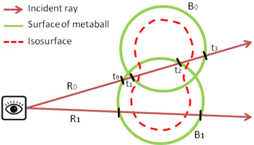
The isosurface of these metaballs will be found using a special ray tracing algorithm. Figure 4.4 shows the sketch map for rendering metaballs. B0and B1are two nearby
meta-balls, and R0is a incident ray intersecting the surface of these two metaballs at{t0, ..., t3}.
We detect the ray-isosurface intersection point from the first interval [t0, t1] to the last
in-terval [t2, t3] using Bézier clipping. This process stops when an intersection is found or
Figure 4.4: A sketch for rendering metaballs.
In each interval, the Bézier curves of the influential spheres are summed into one curve. For instance in the Figure 4.4, the interval [t1, t2] is effected by the B0 and B1 at
the same time, so the Bézier curve f01 in the interval [t1, t2] is constructed by combining
two curves f0 and f1 which represents B0 and B1 respectively. It is simple to combine
multiple Bézier curves, since all we need to do is add each control points di
kbelonging to
each influential spheres; i.e.:
d01k = d0k+ d1k, (k = 0, ..., 6) (4.5)
4.2.3
Bézier clipping
Figure 4.5: A Bézier curve with five control points. (a) is the Bézier curve before clipping, and (b) is the curve after clipping.
as shown in Figure 4.5. The Bézier curve is always inside the convex hull formed by its control points dik. The two intersection points between convex hull and horizontal line
s = T is smin and smax. Therefore, we find [smin, smax] iteratively and finally we can
converge to the root.
In each new interval, we want to obtain new control points for new curve, as shown in Figure 4.5(b). The de Casteljau's Algorithm is utilized here. Also, we use the Jarvis March algorithm to obtain convex hull for curve. These two algorithms will be illustrated in the following section
4.2.4
The de Casteljau's algorithm
The de Casteljau's algorithm is used to obtain new control points for the new curve. If we have the original control points dk(k = 0, ..., n) and the new interval [smin, smax],
we can use this algorithm to get the new control points d′k(k = 0, ..., n). The process of the de Casteljau's Algorithm as below:
1. For any nth order Bézier curve, this algorithm starts with the point set{pk= dk},
which contains exactly n + 1 elements.
2. It then replaces this set with an interpolated set{p′0 = point between p0 and p1 at
distance t, p′1 = point between p1 and p2 at distance t, ..., p′n−1 = point between pn−1 and pn at distance t}, where t is the position we want to find on the original
interval. This set will be 1 element shorter than pk.
3. Step 2 is repeated until there is only one point left, and that point will lie on the original curve, at the same t value.
In this process, the new control points are found at interval [0, t] or [t, 1]. An example is shown on Figure 4.6, assuming point set pk(k = 3).
For the new interval [smin, smax], we run this algorithm two times. In the first time,
we set the smin as t, and find the new control points at interval [t, 1]. Therefore, we get a
Figure 4.6: Finding control points for new curve at interval [0, t] or [t, 1].
the new control points at [0, t]. These new control points are the solution d′k at interval [smin, smax].
4.2.5
Jarvis march algorithm
The property of Bézier curve is that we can use a convex hull to cover the curve, and the convex hull is made by control points. Therefore, we use Jarvis March algorithm to find the convex hull for the curve. Jarvis March algorithm is a simple method that forms edges, and checks that every point is on the same side. The following is the process of algorithm:
1. We assume a virtual first point pv to act as the initial reference.
2. We connect pv and p0 to a line L0, where p0 is the first point of point set P . p0 is
regarded as a judgment point pf ront.
3. We find the biggest angle for L0and Li, where Liis a line constructed by pf rontand
the point pifrom the set P . The point pi will be pushed into hull set H if Lihas the
biggest angle. Then, Libecomes L0, and piturns into pf ront.
4. Step 3 is repeated until pf ront points to h0, where h0 is the first element in hull set
H, and then we find the necessary points of the convex hull which are in the hull
set H.
Figure 4.7: Example of Jarvis March algorithm. The blue line is L0, black lines are the
necessary lines, gray lines and red line are Li, and red line is the line with the biggest angle
calculated with counterclockwise.
4.2.6
Algorithm
We illustrate the process for rendering N metaballs. We render the scene with many rays, and the algorithm is processed for each ray, as shown in Figure 4.8.
In the beginning, we shoot a ray from the view target and perform intersection tests with all the metaballs. The metaball which is intersected have even number of intersection points. We sort the intersection points of all intersected metaballs and construct k intervals. For each interval i, we collect influential metaballs in a set and calculate the control points using de Casteljau's algorithm for these metaballs. To combine multiple Bézier curves, we add each control points dikbelonging to the set of influential metaball and construct a new curve. If all the control points are smaller or bigger than threshold T , then there is no intersection between the convex hull and the horizontal line s = T , so we go to the interval
i+1. Otherwise, we will do the Bézier clipping and find the new interval [smin, smax] until the interval size is small enough (i.e. smaller than ε, where ε is a very small number). The
Figure 4.8: Flow chart of metaballs rendering.
vector scalar t for ray direction is calculated by t = ti + (ti+1 − ti)∗ smin. Therefore,
we can obtain the exact intersect position Ip between ray and metaballs by utilizing the
following equation:
Ip = Vp+ tD, (4.6)
where Vp is the position of view target, and D is the direction vector of the ray.
4.3
GPU-based Ray Tracing With Meshes and Metaballs
To improve the realism, we combine meshes and metaballs in the same scene, and im-plement special ray tracing for these two parts at the same time. We use OpenCL [Khr09] to operate GPU-based parallel computing ability. The kernel function utilized on GPUs allows multiple threads computing simultaneously. Here we set a thread as a ray, and it is in charge of calculating a color of a pixel on the screen.
OpenCL doesn't support calling the same function in a kernel recursively, so we pro-pose an iterative ray tracing method and use a stack to save newly generated reflection ray. We use a stack to save the reflection ray separated from the incident ray. The intensity of ray is reduced, and the ray terminates if its intensity is smaller than the threshold. After
terminating the ray, another ray will be popped from the stack and the intersection will be calculated for it.
The color I of pixel including three parts: color of incident ray Ic, color of reflection
ray Is, and color of refraction ray It. The relation of these three parts as shown in below: I = α∗ Ic+ (1− α) ∗ It+ Is, α∈ [0, 1], (4.7)
where α is the transparency of the intersected object. When α is closer to 0, the object is more transparent.
Figure 4.9: Sketch of ray tracing.
Figure 4.9 is an illustration of ray tracing. The blue area is a transparent object, and the orange bar is the solid object. The different thicknesses of the red arrow represents different intensity of the ray. The computation of the ray is terminated when the intensity of the ray is smaller than the default intensity threshold.
Furthermore, the flow chart of ray tracing algorithm is shown in Figure 4.10. At first, we compute the direction D of incident ray from the view target. We try to find the intersection between the ray and objects, where objects may be meshes or metaballs. In order to find the intersection, we use the ray-metaball intersection to find the nearest intersection point Hmt, and we test intersection between ray and BVH construction of
Figure 4.10: Flow chart of ray tracing.
Hmesh and find out the one which is closer to the view target. We have to compute the
ray-isosurface intersection test if Hmtis closer. It is worth noting that when we compute
the ray-isosurface intersection using the method illustrated in Section 4.2, the algorithm needs to be interrupted once the Hmesh is closer than the absolute position of metaball
interval. This mechanism avoids wrong results from occurring as shown in Figure 4.11. We compute the normal vector n and color Icfor the intersection point, and then we
use the following equation to obtain reflection ray Rs:
Rs = D− 2 ∗ (D · n) ∗ n. (4.8)
The ray Rs will be pushed into stack. If the intersected object is transparent, we
calculate the refraction angle ϕ using the Snell's refraction law:
C sin θ = Ctsin ϕ, (4.9)
where C is the refractive index of incident medium, Ct is the the refractive index of
re-fractive medium, and θ is the angle between n and D. We assume the incident medium is air and the refractive medium is water (or ice). We can use the angle ϕ to obtain refraction ray Rt. Thus, we replace the incident ray D to refraction ray Rtand enter next iteration.
Figure 4.11: The special case occurs when the intersection Hmtis closer to the view target,
but the intersection of isosurface is farer than Hmesh.
The ray would be terminated if the intensity of the ray is smaller than the default inten-sity threshold. In this situation, we pop one ray from the stack and enter the next iteration until there is no element in the stack. Finally, we accumulate all the colors computed by the branch rays into the final color of the pixel.
Chapter 5
Experiments and Discussions
In this section, we show the experimental results from our ice melting method and ray tracing method. We implemented the ice melting simulation and ray tracing using GPUs with OpenCL compute capability 1.1. The experiments were performed on an Intel(R) Core(TM) i7-2600 CPU @ 3.40GHz 3.40GHz with 16.0GB RAM, and NVIDIA GeForce GTX 670. Our development environment was Microsoft Windows 7 Home Premium, and Microsoft Visual Studio 2008. The Nvidia GPU Computing SDK version was 4.20.
We used four benchmarks in our experiments, and we will introduce them in next subsection. These four benchmarks are separately used in different experiments. Below we simply illustrate our experiments:
1. We compared the execution time of ice melting for the same model with different resolutions of voxelization. We want to know the impact of the execution time for different resolutions of voxelization on our system.
2. We compared time used for marching cubes construction and ray tracing between the methods proposed in [IUD10] and ours. The realism are also compared. Iwasaki et al. [IUD10] employed marching cubes to construct both ice model and water droplet, and we separated these two parts and used metaballs to represent the water particles. We are interested in the performance and result of these two methods. 3. We continued to compare the realism between the ice melting methods proposed in
[IUD10] and ours. The method proposed in [IUD10] transforms ice particle to water particle when the particle absorbs enough energy. Then, water droplet appears in place. Our method transfers virtual water volume from high to low via ice particles, and generates water particle when the amount of virtual water volume is too large. 4. We compared the rendering calculation timing between the methods with and
with-out using BVH construction for metaballs. The paper [KSN08] is good for rendering opaque objects using depth peeling. However, the method suffers bad performance when the metaballs are transparent. We used LBVH to build a hierarchy construc-tion, which speeds up the execution time of ray-metaball intersection test.
5. We compared the rendering results between different heat sources acting on the ice. We have two types of heat source: Rectangle and Sphere. Our ice melting simulation method employs two types of heat source. The different shape of heat sources will radiate energy to different directions. We are interested in the rendering results for different heat sources.
5.1
Benchmarks
In our experiments, we perform four benchmarks: Cube, Sphere, Bunny and Dragon. Figure 5.1, 5.2, 5.3, and 5.4 show a series of snapshots for these four benchmarks. Table 5.1 shows the model complexities, and the number of the initial ice particles that belongs to the model.
Figure 5.2: A series of snapshots for Sphere.
Figure 5.3: A series of snapshots for Bunny.