空載光達生產數值高程模型及其精度評估

國

立 交 通 大 學

土 木 工 程 學 系

博

士 論 文

空載光達生產數值高程模型及其精度評估

DTM Generation and Error Assessment for

Airborne LIDAR Data

研 究 生：彭淼祥

指導教授：史天元 博士

空 載 光 達 生 產 數 值 高 程 模 型 及 其 精 度 評 估

DTM Generation and Error Assessment for

Airborne LIDAR Data

研 究 生：彭淼祥

Student:

Miao-Hsiang

Peng

指導教授：史天元 博士

Advisor: Dr. Tian-Yuan Shih

國 立 交 通 大 學

土 木 工 程 學 系

博 士 論 文

A Dissertation

Submitted to Department of Civil Engineering

College of Engineering

National Chiao Tung University

in Partial Fulfillment of the Requirements

for the Degree of

Docotor of Philosophy

In

Civil Engineering

December 2005

Hsinchu, Taiwan, Republic of China

空 載 光 達 生 產 數 值 高 程 模 型 及 其 精 度 評 估

研 究 生：彭淼祥

指導教授：史天元 博士

國 立 交 通 大 學 土 木 工 程 學 系

摘 要

數值地形模型(Digital Terrain Model, DTM)在地理資訊系統應用與分析上是 重要的數據，應用空載雷射掃描技術(或稱為空載光達，Airborne Light Detection and Ranging, LIDAR)測量地形的數值高程數據，其相關技術發展迅速，已經達到 應用階段。空載雷射掃描儀量測地表的反射回訊，獲得三維座標的量測值，量測 點包括了地形面以及非地面的量測點 (如建物、樹木，車輛)，為了生產DTM， 地物的雷射量測點需進一步過濾或分類出來，留下地形面的雷射量測點，進而組 成DTM。關於過濾非地面點的處理，此課題吸引了多方研究的投入，是重要的 研究方向。本研究主要目的，發展出應用多重方式的過濾處理程序，並探討數據 的精度評估。 關於濾除空載光達數據中非地面量測點之研究，目前成果指出，處理崎嶇 的山區地形或高密度植被覆蓋的地區，仍是挑戰性的課題，諸多演算法為了過濾 山區的植被量測點，將地形特徵如地形山脊亦同時被過度平滑濾除，此問題的主 要原因是地物點與地面構成的坡度幾何和背景的陡坡地形坡度幾何，二者的可區 分特性低，本研究提出自適性的過濾演算法，有效的移除背景陡坡地形所干擾的 效應，處理特色在於過濾處理並且能保留地形的特徵。測試區域分別試驗於都市 區域，複雜地類覆蓋與建物的濾除，以及山區植被的濾除，本研究比較不同的過 濾方法，成果顯示本文的方法與商業軟體所使用的自動製程比較，在山區測試數

據組，本文過濾成果與檢核點比較，誤差絕對值的平均22.2 cm，優於自動化程 序25.4 cm，本研究獲得良好的過濾成果。 本研究以山區測試區域(坡度平均26.6°)評估比較兩組光達數據組的特性， 應用地面檢核點(906個檢核數據)分析數據精度，本文分析地形特徵包括地形坡 度，坡向與土地覆蓋類型等因素對於光達高程精度的影響量。文中提出利用光達 數據量化描述土地覆蓋類型的方法，包括植被體積量的估計，局部性地表粗糙度 量測，到達地面的雷射測點平均相鄰點距離，以及植被覆蓋地平角度等評估指標 ，用以量化區別出不同的土地覆蓋類型。應用這些指標推導不同植被型態與光達 高程數據的精度關係。分析成果顯示，光達數據高程精度與這幾個植被型態因子 當中的「植被覆蓋地平角度」，「植被量的估計值」，「局部性地表粗糙度量測 」，「到達地面的雷射測點平均相鄰點距離」等因子有相關聯性，高程精度隨者 這四個因子的變化有統計顯著差異性。「植被覆蓋地平角度因子的三角正切值」 與「到達地面的雷射測點平均相鄰點距離因子」兩個因子乘積，與高程精度具有 高度的線性相關性(迴歸判定係數r2 > 0.9)，高程精度隨不同植被覆蓋型態而變化 。關於地形因子與光達數據高程精度的關係，高程精度隨地形坡度角的變化有統 計顯著差異性。「坡度角的三角正切值」與「到達地面的雷射測點平均相鄰點距 離」兩個因子乘積，與高程精度亦具有高度的線性相關性(迴歸判定係數r2 = 0.9) ，乘積的數值越大(地形越陡)，高程誤差越大。另外，有一組數據具有附加的交 錯飛行掃描數據，以本文測試數據而言，交錯飛行，能降低坡向因子對於高程精 度的影響量。

DTM Generation and Error Assessment for

Airborne LIDAR Data

Student: Miao-Hsiang Peng Advisor: Dr. Tian-Yuan Shih

Department of Civil Engineering

National Chiao Tung University

ABSTRACT

Airborne light detection and ranging (LIDAR) technology has become a leading method for producing digital terrain models (DTMs) that are important to many GIS-related analyses and applications. In generating a digital terrain model, removing non-terrain measurements from LIDAR datasets has proven to be an important task. In this dissertation, a series of filters are developed to remove non-terrain LIDAR measurements.

It is difficult to accurately extract the terrain surface in areas of rugged relief or discontinuous topography. This research applies adaptive techniques to remove the effects of background relief. The terrain data are preserved, while non-terrain points are removed. The proposed method can discriminate effectively between terrain and non-terrain measurements, and has been tested for urban and mountainous areas. The filtered results from the proposed method are compared to traditional automatic techniques. The results indicate that the proposed method produces a better digital terrain model.

An accuracy assessment of two LIDAR-derived elevation datasets was conducted in areas of rugged terrain (average slope 26.6°). Data from 906 ground checkpoints in various land-cover types were collected in situ as reference points. Analysis of the accuracy of LIDAR-derived elevation as a function of several factors including terrain slope, terrain aspect, and land-cover types were conducted. This paper attempts to characterize vegetation information derived from LIDAR data based on variables such as canopy volume, local roughness of point clouds, point spacing of LIDAR ground returns, and vegetation angle. This information was used to evaluate the accuracy of elevation as a function of vegetation type. The experimental results revealed that the accuracy of elevation was considerably correlated with five factors: terrain slope, vegetation angle, canopy volume, local roughness of point clouds, and point spacing of LIDAR ground returns. The results show a linear relationship between the elevation accuracy and the combination of vegetation angle and the point

spacing of ground returns (r2 > 0.9). The combination of vegetation angle and point

spacing of ground returns explains a significant amount of the variability in elevation accuracy. Elevation accuracy varied with different vegetation types. The elevation accuracy was also linearly correlated with the product of the point spacing of ground

returns and the tangent of the slope (r2 = 0.9). A greater product value implies a

greater elevation error. In addition, with regard to terrain aspect, one dense dataset with extra cross-flight data revealed a lesser impact of aspect on elevation accuracy.

TABLE OF CONTENTS

Abstract in Chinese ... I Abstract ...III TABLE OF CONTENTS...V LIST OF TABLES ... VII LIST OF FIGURES ...IX LIST OF ACRONYMS... XII

CHAPTER ONE: INTRODUCTION...1

1.1 Background ...1

1.2 Statement of the Problem...3

1.3 Contributions...5

1.4 Thesis Outline ...6

CHAPTER TWO: LITERATURE REVIEW ...7

2.1 Algorithms for DTM Generation ...7

2.2 Error Assessment for LIDAR-derived DTM ...10

CHAPTER THREE: DIGITAL TERRAIN MODEL GENERATION ...14

3.1 Terrain filtering concept ...14

3.2 Slope-based filter ...18

3.3 Directional steepest-descent filter...21

3.4 Adaptive directional steepest-descent filter ...26

3.5 Adaptive directional elevation-difference filter...27

3.6 Determination of search radius ...29

3.7 Filtering by multiple filtering procedures ...30

3.8 Algorithm implementation...33

3.10 Experiment and Evaluation...45

CHAPTER FOUR: ERROR ASSESSMENT AND DTM VALIDATION...63

4.1 Characterization of vegetation information ...63

4.2 Descriptions of land-cover types by vegetation information...67

4.3 Analysis of point spacing of LIDAR ground returns...76

4.4 Analysis of terrain slope ...76

4.5 Verifying the distribution of checkpoints...77

4.6 Assessing errors using checkpoints ...78

4.7 Elevation error and vegetation type ...82

4.8 Elevation error and point spacing of LIDAR ground returns ...89

4.9 The combination effect of vegetation angle and point spacing ...91

4.10 Elevation error and terrain form ...93

4.11 Comparisons between photogrammetry and LIDAR...99

CHAPTER FIVE: CONCLUSIONS AND RECOMMENDATIONS...108

LIST OF TABLES

Table 3.1 Statistics of terrain slopes of test site ...37

Table 3.2 LIDAR collection parameters of high relief site...39

Table 3.3 Land-cover classes and their descriptions...41

Table 3.4 The accuracy of multiple filtering results ...52

Table 3.5 Accuracy of DTM in bald earth areas (H = 1100 m, error in cm) ...57

Table 3.6 Accuracy of DTM in bald earth areas (H = 1800 m, error in cm) ...58

Table 3.7 Accuracy of DTM for automatic processing with manual edits (H = 1100 m, error in cm)...59

Table 3.8 Accuracy of DTM for automatic processing (H = 1800 m, error in cm) ..60

Table 3.9 Accuracy of DTM for multiple-filter processing (H=1100m, error in cm) ...61

Table 3.10 Accuracy of DTM for multiple-filter processing (H=1800m, error in cm) ...62

Table 4.1 Summary of 29 tree height measurements from field survey ...67

Table 4.2 Summary statistics of results for H = 1100 m dataset...69

Table 4.3 Summary statistics of results for H = 1800 m dataset...70

Table 4.4 Relationship between vegetation information for H = 1100 m dataset...74

Table 4.5 Relationship between vegetation information for H = 1800 m dataset...75

Table 4.6 Number of checkpoints by slope class and vegetation angle...78

Table 4.7 Accuracy of terrain model for H = 1100 m dataset (error in cm) ...80

Table 4.8 Accuracy of terrain model for H = 1800 m dataset (error in cm) ...81

Table 4.9 Mean signed error...82

Table 4.11 Elevation error by land-cover class (error in cm) ...83

Table 4.12 Elevation error related to vegetation type by reference canopy volume.85 Table 4.13 The elevation error and local roughness on checkpoints ...87

Table 4.14 Relationship between elevation error and vegetation angle...88

Table 4.15 Regression of elevation error and vegetation angle ...88

Table 4.16 Elevation error and mean distance to the nearest LIDAR point ...90

Table 4.17 Regression of elevation error and mean distance to the nearest LIDAR point ...90

Table 4.18 Relationship between elevation error and the product of distance to nearest LIDAR point and the tangent of the elevation angle...92

Table 4.19 Regression of elevation error and the product of distance to nearest LIDAR point and the tangent of the elevation angle ...92

Table 4.20 Elevation error by reference slope ...94

Table 4.21 Regression of elevation error and slope...94

Table 4.22 Relationship between elevation error and the product of the mean distance to the nearest LIDAR point and the tangent of the slope...96

Table 4.23 Regression of elevation error and the product of the mean distance to the nearest LIDAR point and the tangent of the slope...96

Table 4.24 Elevation error by aspect class...98

Table 4.25 The differences of DSM in landslide rock (discrepancies between photogrammetry and LIDAR)...105

Table 4.26 The accuracy of DTM by manual measurement in stereo-mode environment ...106

LIST OF FIGURES

Figure 3.1. An example of gentle terrain relief...16

Figure 3.2. The profile has gentle terrain relief. ...16

Figure 3.3. Filtering examples of global thresholding...16

Figure 3.4. Filtering by local thresholding technique. ...17

Figure 3.5. Filtering example of local thresholding...18

Figure 3.6. Steepest descent, defined as the minimum angle unobstructed...19

Figure 3.7. An example of large terrain relief...20

Figure 3.8. Six results of slope-based filtering. ...21

Figure 3.9. Azimuth angle D is measured clockwise from north...23

Figure 3.10. Comparison between slope-based and directional steepest-descent filter. ...24

Figure 3.11. Comparison of profile between slope-based and directional steepest-descent filter. ...26

Figure 3.12. The steepest-descent is revised by removing the background slopes...27

Figure 3.13. Finding the lowest point progressively...28

Figure 3.14. Taking p as a center, relief spots are further selected and constitute set T. ...30

Figure 3.15. Flowchart of the multiple filtering algorithm...31

Figure 3.16. Sample profile. ...32

Figure 3.17. The elevation-differences values of the sample profile...33

Figure 3.18. The steepest-descent values of the sample profile...33 Figure 3.19. High-relief site is located in central Taiwan affected by the Chi-Chi

Earthquake. ...38

Figure 3.20. Slopes distribution over the test site...38

Figure 3.21. Distribution of ground checkpoints in study area...42

Figure 3.22. Field and aerial photos of the surveyed site. ...45

Figure 3.23. Effect of varying initial radius on errors, ...46

Figure 3.24. Effect of varying initial radius on errors, ...47

Figure 3.25. The DTM generation results for the urban area. ...50

Figure 3.26. The filtering errors for sample sites...51

Figure 3.27. The comparisons of DTMs for H = 1100 m. ...56

Figure 3.28. The comparisons of DTMs for H = 1800 m. ...56

Figure 4.1. The greatest vegetation angle is defined as the maximum angle of the line-of-sight unobstructed to a specified distance L. ...66

Figure 4.2. Azimuth angle D is measured clockwise from north...66

Figure 4.3. Comparison of shaded relief maps for tea farm A...77

Figure 4.4. MAE error of both datasets, using various types of land-cover. ...84

Figure 4.5. Elevation error as a function of canopy volume...85

Figure 4.6. Elevation error as a function of local roughness on checkpoints. ...87

Figure 4.7. Elevation error as a function of vegetation angle...89

Figure 4.8. Elevation error as a function of the mean distance...91

Figure 4.9. Elevation error as a function of the product of the mean distance to nearest LIDAR point and the tangent of the vegetation angle. ...93

Figure 4.10. Elevation error as a function of slope...95

Figure 4.11. Elevation error as a function of product of the mean distance to the nearest LIDAR point and the tangent of the slope...97

Figure 4.12. Mean absolute error as a function of terrain aspect,...99

Figure 4.14. The comparisons of contours...103 Figure 4.15. The comparisons of DTMs from LIDAR-derived vs.

LIST OF ACRONYMS

DEM Digital Elevation Model

DSM Digital Surface Model

DTM Digital Terrain Model

FEMA Federal Emergency and Management Agency

GIS Geographic Information Systems

GPS Global Positioning System

IDW Inverse Distance Weighting

LIDAR Light Detection And Ranging

MAE Mean Absolute Error

RMSE Root Mean Square Error

RTK Real-Time-Kinematics

TIN Triangulated Irregular Network

CHAPTER ONE: INTRODUCTION

1.1 Background

Airborne LIght Detection And Ranging (LIDAR) is an active sensor that captures topographic data rapidly, economically and accurately. Consisting of a laser distance measurement, a scanning mirror, and an integrated GPS/INS system, airborne LIDAR has recently become a leading method for producing Digital Terrain Models (DTMs), (Ackermanm, 1999; Huising and Gomes Pereira, 1998; Kraus and Pfeifer, 1998; Baltsavias, 1999a; Wehr and Lohr, 1999; Maas, 2002).

Commercial LIDAR system designs have been based on the work done by NASA. Generally, there are two types of LIDAR systems: bathymetric systems work over water and topographic systems work over land. The wavelength for topographic LIDAR sensor is between 1.053 and 1.064 μm (the infrared portion of the spectrum), while airborne bathymetric LIDAR sensors use the blue/green portion of the spectrum. The pulse rates have increased with development of technology. The pulse rate, (measured in kilohertz, kHz) is the number of bursts of light per second; a 2 kHz system generates 2,000 pulses of laser energy in one second. Early systems offered pulse rates on 2 kHz to 7 kHz, while modern systems come with pulse rates of 25 kHz to 83 kHz. Higher pulse rates mean increased resolution. The spatial resolution varies depending on the pulse rate, flying altitude, and aircraft speed (Baltsavias, 1999b). Two distinct techniques of LIDAR have been developed: small footprint, time-of-flight laser altimetry and large footprint, waveform-digitizing techniques that analyze the full return waveform to capture a complete elevation profile within the target footprint (Flood, 2001). A typical laser beam used in a

small footprint LIDAR sensor has divergences of 0.2-to 0.33-mrad.

Airborne LIDAR can operate at night and is less affected by weather conditions than aerial photography, making it suitable for emergent mapping. The US Federal Emergency and Management Agency (FEMA) utilized airborne LIDAR to create digital terrain models for hydraulic modeling of floodplains, digital terrain maps, and other National Flood Insurance Program products for flood mitigation applications.

Most LIDAR sensors collect both range and intensity of the returned signal and information of multiple returns for each pulse. The multiple returns may be useful to categorize vegetation. Pfeifer et al. (2001) observed that 85% of the first and last pulses showed no difference in a sample case of building areas, whereas for the wooded areas only 20% of the two returns were identical. Some overviews of airborne LIDAR technology can be found (Maune, 2001; Baltsavias, 1999b; Hu, 2003; Wehr and Lohr, 1999).

The Netherlands is the first country to utilize airborne LIDAR to establish a

nationwide digital elevation model with a density of 1 point per 16 m2 (Huising and

Gomes Pereira, 1998; Crombaghs et al., 2000). In addition to terrain mapping, airborne LIDAR can also be applied in the reconstruction of 3-D building models (Haala et al., 1998, 1999; Maas and Vosselman, 1999; Brenner, 2000; Vosselman and Dijkman, 2001). Hyyppä et al. (2001) reported on the use of small-footprint LIDAR in Finland to detect characteristics of individual trees such as their height, location, and crown dimensions. In the sparse boreal forest, where more than 30% of pulses reach the ground, a segmentation-based method retrieved stem volume estimates of the mean height, basal area, and stem volume with standard errors of 9.9%, 10.2%, and 10.5%, respectively. A few papers have used small-footprint LIDAR to infer vegetation characteristics and have achieved prediction of tree height and stem volume (Means et al., 2000; Næsset, 1997a; Næsset, 1997b).

Even though this technology is accepted as a tool for terrain mapping, the processing of LIDAR data is still in the situation of development. The two major problems of data processing are the elimination of systematic errors and the processing to remove non-terrain points from LIDAR datasets (Huising and Gomes Pereira, 1998). Determining whether a returned pulse is a terrain point or non-terrain cover is still an intense research topic. Most algorithms have difficulty accurately extracting the terrain surface, especially in areas of dense wooded cover, rugged relief or discontinuous topography.

1.2 Statement of the Problem

The most common use of LIDAR data is to generate DTMs, which are important for many GIS-related analysis and applications. To generate a DTM, the terrain points need to be identified, and the non-terrain points (trees, buildings, and vehicles, etc.) removed from the LIDAR measurements. Many algorithms have been developed to remove non-terrain points and generate DTMs (Kraus and Pfeifer, 1998; Pfeifer et al., 1999; Vosselman, 2000; Axelsson, 2000; Elmqvist, 2001; Briese et al., 2002; Brovelli et al., 2002; Wack and Wimmer, 2002; Hu, 2003; Zhang et al., 2003; Sithole and Vosselman, 2004). However, the filtering processing of LIDAR data is still in a phase of development.

There are two basic errors in filtering LIDAR measurements. A Type I error is one that removes bare-Earth points mistakenly; Type II errors involve accepting non-terrain points as terrain measurements. While filtering processing, a trade-off is involved between making Type I and Type II errors. Variety of terrain type and land-cover type may influence the performance of filtering algorithms (Sithole, 2001; Sithole and Vosselman, 2003). Determining filtering parameters in terms of terrain

information is somewhat subjective. The choice of proper parameters may be problematic. It is difficult to detect all non-terrain objects of various sizes using a fixed parameter.

The focus of this research is on developing and implementing algorithms for automatic extraction of topographic surface. The robustness of performance and feature preservation of filtering result are emphasized.

Though a general understanding of the accuracy of LIDAR is known, too few empirical studies exist for assessing the accuracy of DTMs derived from LIDAR data. Gomes Pereira and Janssen (1999) used a low-flight-altitude (240 m) dataset to evaluate LIDAR-derived Digital Elevation Models (DEMs) and found that root-mean-square error (RMSE) varied from 8 to 15 cm in flat regions, and from 25 to 35 cm in sloped terrain. Typical elevation accuracies of LIDAR-derived DEMs have 15 cm RMSE over non-forested flat surfaces (Hodgson and Bresnahan, 2004). Hodgson et al. (2003) showed that land-cover types and terrain slope substantially affected the elevation accuracy determined from leaf-on LIDAR data in North Carolina. Accordingly, evaluating LIDAR accuracy based on both land-cover types and terrain characteristics is necessary.

The vegetation types for collecting reference points are commonly divided into basic land-cover categories such as tall weeds, brush/low trees, and forests. Raber et

al. (2002) developed an adaptive LIDAR vegetation point removal process. They

used an algorithm adaptively adjusting the parameters based on a vegetation map. There is a need for research efforts in quantifying the accuracy of LIDAR data collected under various collection parameters, filtering processes, and geography conditions. This study evaluated a method to identify vegetation characteristics based on LIDAR data. The derived vegetation information was factored into the evaluation of the impact of vegetation types on the accuracy of LIDAR-derived

elevation. This research considers some quantitative descriptors such as vegetation angle, canopy volumes and LIDAR-derived tree height, to characterize the relationship between elevation accuracy and the types of vegetation. One distinctive aspect of this study is its use of LIDAR data points to derive information about vegetation types in terms of descriptors.

1.3 Contributions

The following novel contributions were developed to achieve the research objectives:

* This research developed a multiple-filtering framework to remove non-terrain LIDAR measurements to generate DTMs. An adaptive directional steepest-descent filter is proposed. The proposed algorithm is suited to efficiently separate terrain and non-terrain LIDAR data in both urban and mountain areas. This work also proposed an adaptive directional elevation-difference filter to remove large objects such as very large buildings. The selections of the filtering parameters are very important. The proposed multiple-filtering framework is highly automatic to adaptively adjust the parameters.

* The research proposed to characterize vegetation information derived from LIDAR data base on variables such as canopy volume, local roughness of point clouds, point spacing of LIDAR ground returns, and vegetation angle. This information was used to evaluate the accuracy of elevation as a function of vegetation type. Two sets of LIDAR-derived elevation were used to evaluate the impact of terrain slope, terrain aspect, and land-cover type on elevation accuracy.

The framework of accuracy assessment is also presented.

1.4 Thesis Outline

In Chapter 2, a literature review on related filtering processes and quality assessment is reported. Chapter 3 describes the development of a multiple-filtering procedure for DTM generation. In Chapter 4, the error factors of the DTM are discussed. Conclusions are presented in Chapter 5, followed by suggestions for future research.

CHAPTER TWO: LITERATURE REVIEW

2.1 Algorithms for DTM Generation

LIDAR acquires a three-dimensional cloud of points with irregular sampling. The measurements hit on objects such as buildings, vehicles, vegetation, and bald terrain. To generate a DTM, the core task involves the separation of non-terrain points from LIDAR datasets. This task is referred to as filtering, classification, non-ground measurements removal. The filtering task dominates the topic of DTM generation. A number of algorithms have been reported in the literature, but there are a number of conditions that make filtering a very difficult problem. DTM generation from LIDAR data has proven to be a challenging task.

Kraus and Pfeifer (1998, 2001) utilized linear least squares interpolation iteratively to remove tree measurements and generate DTMs in forest areas. The least squares interpolation is based mainly on calculating the residuals, i.e., the distance from the surface to the measurement points. It is assumed that terrain points are likely to have negative residuals, whereas non-terrain points are more likely to have positive residuals. These residuals are used to compute weights. Points with large negative residuals have maximal weights and they attract the surface. Similar methods have been adopted by Lohmann et al. (2000). Pfeifer et al. (2001) extended this method by a hierarchical strategy to assemble data from coarse to fine. Lee and Younan (2003) used a modified linear prediction technique, followed by adaptive processing and refinement. However, this method fails to model terrain with steep slopes and large variability. In addition, extreme low points can be easily misclassified as terrain points as a result of the negative errors.

Kilian et al. (1996) used morphological filters to eliminate non-terrain points. Typically these filters need to predefine a search window size. These filters may have problems with dense forest canopy or large buildings. If a small window size is used, large-sized buildings cannot be removed. On the other hand, larger window size causes the filter to over-remove terrain points or chop off hills. Kilian et al. (1996) suggested using a series of windows to progressively filter the terrain.

Petzold et al. (1999) proposed a filtering algorithm. A rough terrain model is calculated by the lowest points found in a moving window of a rather large size. All points with a height difference exceeding a given threshold are filtered out, and a more precise DTM is calculated. This step is repeated several times by reducing the window size. The final window size and the final threshold have great influence on the results: small window size leads to points on large buildings remaining, while a high threshold in the final step leads to non-terrain points being classified as terrain points. Therefore, the parameters depend on the terrain variation and have to be adjusted for flat, hilly and mountainous regions.

The concept of resizing window size was adopted by Zhang et al. (2003, 2005); they proposed a progressive morphological filter. By gradually increasing the window size of the filter and using elevation difference thresholds, the non-terrain points are removed, while terrain points are preserved.

Lohmann et al. (2000) compared two algorithms, namely the use of linear prediction and the use of dual rank filters. The use of linear prediction showed satisfactory results in forest areas, whereas areas with steep terrain showed problems. The linear prediction filter needs to be improved by being locally adapted to the shape of the terrain (Lee and Younan, 2003). The dual rank filter is a mathematical morphology filter which is applied to a grayscale image. Dual rank filters need to be improved through interactive control and some pre-knowledge to properly set the

necessary parameters.

Vosselman (2000) proposed a slope-based filter. This method was commonly applied for DTM generation from LIDAR data. A measurement is classified as a terrain point if the height differences of this measurement point and any other point within a given circle are smaller than a predefined threshold. Choosing a threshold of too small height results in removing some detail of the terrain or cutting hill peaks; too large a threshold results in preservation of non-terrain points. Furthermore, the fixed threshold procedure limits the use of slope-based filter to terrain with gentle slopes. This technique will give satisfactory results only when non-ground objects (trees, buildings, etc.) and background terrain slopes are distinct and are uniform throughout the full coverage.

The next parameter of the filter is the radius of search region. The region size should be large enough to enclose the larger non-ground objects, such as buildings, but not so large as to cover different terrain aspects (i.e., ridges should not be crossed). Small search regions tend to cover uniform background slopes. Large regions tend to have larger topographical undulations than smaller regions. Adaptive techniques are required to overcome the effects of nonuniformities in background slopes. Slope-based filter has been shown to be equivalent to the erosion operator in morphology. Sithole (2001) has attempted to improve this filter.

Axelsson (1999, 2000) described an adaptive TIN (Triangulated Irregular Network) model to process ground points in dense urban areas where discontinuities may occur. A course TIN is formed based on seed points selected from low points. The course TIN iteratively adds more points if their parameters are below threshold values. The problem with adaptive TIN is that it is difficult to detect various sizes of non-ground objects by using a fixed parameter. Raber et al. (2002) showed an adaptive vegetation removal process. The different thresholds were adaptively given

based on a vegetation map for various land cover types.

2.2 Error Assessment for LIDAR-derived DTM

The elevation accuracy of LIDAR-derived DTM is routinely quoted as 15 cm. The quality of the final DTMs was influenced by the following components:

* elevation error from the system measurement, * horizontal error from the system measurement,

* misclassification of terrain points as non-terrain points, * misclassification of non-terrain points as terrain points, and

* interpolation error introduced into DTM derived from clouds of points.

1. Sources of X-Y-Z error

The sources of positional (X-Y-Z) error in the collection processing can be grouped according to (1) the laser instrument, INS and GPS, (2) the process of measuring from the air, and (3) the target surface causing measurement to be influenced by the type of ground coverage and the terrain slope. A discussion of sources of systematic and random errors can be found in Huising and Gomes Pereira (1998).

Factors that affect the accuracy of LIDAR measurements include the following: (1) instrument-related factors such as the measurement accuracy of the laser range finder, the GPS receiver, the INS and the scanner (Wehr and Lohr, 1999); (2) calibration errors caused by misalignment between instrument components; (3) data collection parameters, such as the flying height and the width of the field of view of the scanner, which can both be reduced to improve the accuracy of LIDAR measurements (Baltsavias, 1999b); (4) GPS data quality, such as GPS PDOP value,

satellite phase RMSE and the base station distance separation, and (5) atmospheric refraction error.

2. Mapping sources error

A characteristic of elevation error for terrain mapping is the relationship with terrain slope (Hodgson and Bresnahan, 2004). Typically, planimetric accuracy is lower than height accuracy of LIDAR measurement. A horizontal error on a flat surface will have no influence on vertical errors, while for inclined slopes the horizontal error in the observation may introduce extra error in the elevation value. The amount of elevation error introduced is a function of terrain slope (Hodgson and Bresnahan, 2004):

Elevation Error = tan (slope) × Horizontal error (2.1)

3. LIDAR point classification error

Sithole and Vosselman (2003) evaluated the performance of eight filtering algorithms. Twelve datasets were processed to test these filters, and it was found that all the filters performed well in smooth rural landscape. However, complex urban areas and rough terrain with vegetation still pose challenges to automating the process of generating DTMs.

Pfeifer et al. (2001) presented an iterative robust filtering approach (using linear prediction based on the software SCOP++). With the OEEPE test data sets the suitability of the algorithm demonstrated the vertical accuracies of three areas in RMSE of 11 cm and one area in RMSE of 48 cm.

Raber et al. (2002) conducted an adaptive technique to create DTMs through LIDAR-derived vegetation type information. The adaptive technique creates a superior DTM compared to DTMs created by automatic processes. They

demonstrated the vertical accuracies of using the adaptive optimized method in RMSE of 29 cm and using automatic with human edits in RMSE of 45 cm.

4. Interpolation Error

Interpolation error is semi-systematic. It is related to the density of mass points, the use of extra data such as breaklines, the use of data structure, and interpolation techniques. Point spacing between LIDAR returns is the result of collection parameters, including (1) flying altitude and speed of the aircraft, (2) the pulse rate, and (3) the scan angle. Lloyd and Atkinson (2002) compared the Inverse Distance Weighting and kriging interpolation techniques. They showed that the advantages of kriging with a trend model were more accurate when the number of data points decreases. It should be noted that the significant differences between varies of the interpolation of gridded DTMs were suspected because standard deviation in elevation error ranged from only 10.9 cm to 12.8 cm (decrease less than 2 cm) in their study. The interpolation methods of Inverse Distance Weighting and kriging can be found in Peng and Shih (2002). Smith et al., (2004) showed that the increase in errors at rough resolutions (4 m grid comparison on a 1 m grid) were of the order of 50–80 cm. These two studies did not reveal the interaction impact of terrain slope and the density of mass points on the accuracy of LIDAR-derived elevation. Hu (2003) used a variety of data structures to compose DTMs resulting in non-significant differences in quality. Hodgson and Bresnahan (2004) also found that additional error introduced by interpolation is low and does not have a major impact on the total error budget (adding up to 3.3 cm to any land-cover class).

5. Quality Control Checkpoints

checkpoints. At lease 20 three-dimensional QC checkpoints are collected in each of five land-cover categories. The examples of land-cover categories: (1) grass (sand, rock, lawns, golf courses), (2) weeds and crops, (3) scrub (brush land and low trees), (4) forest, (5) built-up areas with dense man-made structures.

6. Empirical Study of LIDAR Error

Kraus and Pfeifer (1998) assess a dataset collected at 1000 m flying altitude. In flat terrain, comparing 466 ground checkpoints with LIDAR data showed that the RMSE was 25 cm. After further improvements in the data processing, an accuracy of 10 cm was achieved.

Ahokas et al. (2003) evaluated height errors of LIDAR datasets collected at different flying altitudes, and found that the higher the flying altitude, the larger the height error. For asphalt surfaces a standard deviation of 10 cm is obtainable from H = 550 m.

Hodgson et al. (2003) reported accuracy from 3.4-m post spacing dataset collected in leaf-on conditions. This study found an elevation error of 33 cm in low grass and 153 cm in scrub. Errors in low grass and high grass were much smaller than those in heavily vegetated canopies.

The comparisons between LIDAR and photogrammetry can be found in Baltsavias (1999c); Kraus and Pfeifer (1998); Adams and Chandler (2002). Other studies regarding estimating relative LIDAR accuracy by comparing overlapping datasets include Behan (2000), Burman (2000), Vosselman and Maas (2001), Latypov (2002), Maas (2002), and Crombaghs et al. (2000, 2002), Liu (2005).

CHAPTER THREE: DIGITAL TERRAIN MODEL

GENERATION

To generate a digital terrain model of the bare Earth, the non-terrain points must be filtered out from LIDAR datasets, a process sometimes referred as vegetation removal, classification, filtering, or DTM generation. It is difficult to extract the terrain surface completely with complex land-cover solely using a single algorithm. The multiple-filtering approaches developed for DTM generation are described below. The quality assessment of the filtering results for several datasets was conducted.

3.1 Terrain filtering concept

In order to eliminate non-terrain points, every filter needs to make an assumption to mathematically define what a terrain point is. I developed algorithms to analyze the geometric characteristics, such as slopes and differences, of a point relative to its neighboring points. The concepts adopted in this research include the following:

* The lowest point is more likely to be a ground measurement. The lower the point, the larger probability to be a terrain point (Petzold et al., 1999; Axelsson, 2000).

* Variation of the slope at the edge of non-terrain objects is significant than terrain points of flat ground (Vosselman ,2000; Sithole, 2001).

* Since terrain points have lower elevations than non-terrain points, it is able to separate terrain points with other objects by using elevation differences.

Local lower points are usually the candidate terrain points, and local higher points are likely building roof or tree points. This idea was commonly applied for filtering algorithm. Petzold et al. (1999) proposed a filtering algorithm based on finding local low points in moving filtering windows of varying sizes. Kraus and Pfeifer (1998) developed algorithm based on the linear prediction. Low points have maximal weights and they attract the prediction surface. High points with minimal weights are eliminated. Another commonly used algorithm to find minimum values is a mathematical morphology filter which is applied to a raster image.

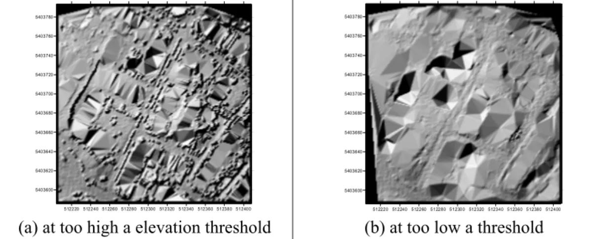
Figure 3.1 and 3.2 show a cross section of LIDAR points. The dashed line in Figure 3.2 indicates the elevation of the threshold. High points should be filtered and low points should be kept. Thresholding is a synonymous term for filtering. The most important task in performing filtering is the choice of an appropriate threshold level. I distinguish two approaches of thresholding techniques. Global thresholding use the fixed threshold value. Local thresholding examine relationships between elevations of neighboring points to adapt the threshold according to the terrain variation for different terrain regions. The approach of fixed global thresholding may be satisfactory when the elevation has relatively gentle variations throughout the full coverage. Figure 3.3 (a) and (b) show examples of the results of poorly chosen thresholds. In Figure 3.3 (a), the elevation threshold is chosen too high, resulting in some non-terrain points such as trees remaining. In Figure 3.3 (b), the elevation threshold is chosen too low, resulting in some terrain details unwanted filtered.

512220 512240 512260 512280 512300 512320 512340 512360 512380 512400 5403600 5403620 5403640 5403660 5403680 5403700 5403720 5403740 5403760 5403780

Figure 3.1. An example of gentle terrain relief.

Figure 3.2. The profile has gentle terrain relief.

512220 512240 512260 512280 512300 512320 512340 512360 512380 512400 5403600 5403620 5403640 5403660 5403680 5403700 5403720 5403740 5403760 5403780

(a) at too high a elevation threshold

512220 512240 512260 512280 512300 512320 512340 512360 512380 512400 5403600 5403620 5403640 5403660 5403680 5403700 5403720 5403740 5403760 5403780

(b) at too low a threshold Figure 3.3. Filtering examples of global thresholding.

Profile 1

One approach to local thresholding is to subtract a local trend surface from the original elevation data. We may implement this by using erosion operation of morphological processing to calculate a moving region minimum. For a LIDAR measurement p(x,y,z), the erosion of elevation z at x and y is defined as

(3.1)

The erosion output ep is the minimum elevation value in the neighborhood of

point p. By comparing each elevation value to its eroded trend surface, remove non-terrain objects if it is much above (or above a given threshold such as 0.3 m) the eroded surface.

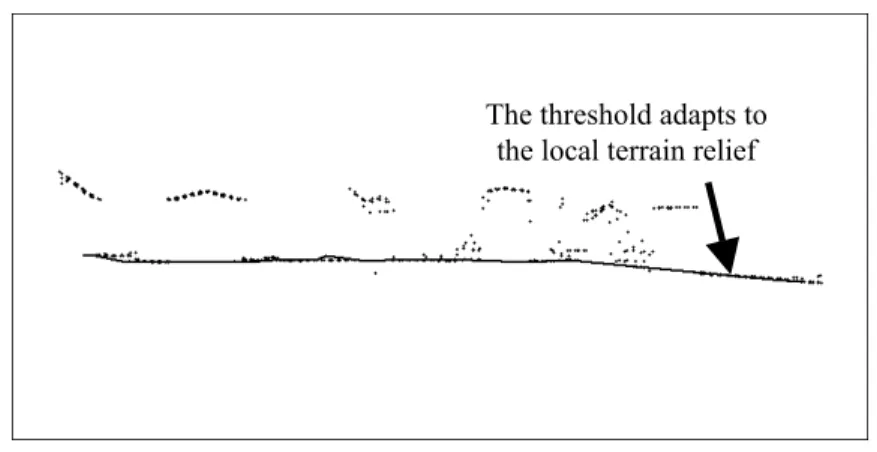
Figure 3.4 shows the eroded surface by applying an erosion operation with a window size of 10 m. The windows size in erosion operation should be large enough to enclose an object such as a large building completely. Note large building objects large than the window size are remained by erosion (Figure 3.5). This choice of proper size for the window may be problematic when coverage contains large buildings of variable size.

Figure 3.4. Filtering by local thresholding technique.

The eroded trend surface was calculated from a moving window minimum. The window size is set to 10 meters.

The threshold adapts to the local terrain relief

512220 512240 512260 512280 512300 512320 512340 512360 512380 512400 5403600 5403620 5403640 5403660 5403680 5403700 5403720 5403740 5403760 5403780

Figure 3.5. Filtering example of local thresholding.

The window size must be set with respect to the objects size: otherwise, large building objects large than the window size are remained.

The variety of landscapes to be performed filtering requires different approaches. There is not a single optimal method of filtering for all conditions till today. I developed a series of filtering techniques: (1) Directional steepest-descent filter examine the steepest slope in the different directions to counter the directional effects and improve the slope-based filter; (2) Adaptive techniques examine relationships between slopes (or height differences) of neighboring points to adapt the threshold according to the examined slopes (or height differences) statistics; (3) Automatically determination of search size, it may match for different terrain.

3.2 Slope-based filter

non-ground objects. Assuming that the slope in natural terrain should change gradually. Whereas on the edge of non-ground objects, the slopes and elevation differences between the ground and non-ground points should be larger than those between ground points.

A measurement is classified as a terrain point if the steepest slope of this measurement point and any other point within a given circle are smaller than a predefined threshold. In words: a point p is classified as a terrain point if there is no other point i such that the slope between these points is larger than the allowed maximum slope (Figure 3.6). To find the steepest slope by a search distance from the measurement point p is in the form

        − + − − = =1~ ( )2 ( )2

max

where points (xi,yi,zi) represent point p’s neighbors within a radial distance L of

a given circle, and n is the total number of p’s neighbors.

Figure 3.6. Steepest descent, defined as the minimum angle unobstructed.

The selection of the searching window size L is important when using this filter. If a small window size is used, large-sized buildings cannot be removed. On the

other hand, larger window size causes the filter to over-remove terrain points or chop off hills. Figure 3.7 shows an example of large terrain relief. Figure 3.8 shows the results of slope-based filtering for six cases, and their parameters including search window and slope threshold. The larger search windows the terrain feature is more eroded.

1186100 1186150 1186200 1186250 1186300 1186350 2564800 2564850 2564900 2564950 2565000 2565050 2565100 1186100 1186150 1186200 1186250 1186300 1186350 2564800 2564850 2564900 2564950 2565000 2565050 2565100 1186100 1186150 1186200 1186250 1186300 1186350 2564800 2564850 2564900 2564950 2565000 2565050 2565100

(a) Search radius: 3 m Threshold: 100% (45°) (b) Search radius: 3 m Threshold: 58%(30°) (c) Search radius 3 m Threshold: 27%(15°) 1186100 1186150 1186200 1186250 1186300 1186350 2564800 2564850 2564900 2564950 2565000 2565050 2565100 1186100 1186150 1186200 1186250 1186300 1186350 2564800 2564850 2564900 2564950 2565000 2565050 2565100 1186100 1186150 1186200 1186250 1186300 1186350 2564800 2564850 2564900 2564950 2565000 2565050 2565100 (d) Search radius 5 m Threshold: 100% (45°)

(e) Search radius 5 m Threshold: 58%(30°)

(f) Search radius 5 m Threshold: 27%(15°) Figure 3.8. Six results of slope-based filtering.

3.3 Directional steepest-descent filter

Based on the idea of slope-based filter, this paper develops an algorithm to improve the directional effect of slope-based filter. The directional steepest descent filter relies on the steepest slope in the four directions (the same rule as in eight directions or sixteen directions) within a radial distance from a point (Figure 3.9). The steepest descent is similar to equation 3.2.

        − + − − = =1~ ( )2 ( )2 ) tan(

max

where points (xi,yi,zi) represent point p’s neighbors along an azimuth D within a

radial distance L, and n is the total number of p’s neighbors in the direction D. Figure 3.9 shows the two-dimensional search-space spanned by two specific azimuthal angles and a distance.

The algorithm is to take p as a center and calculate the steepest descent to any other points reached within the four areas. The areas of directions 45 and 225 degrees are taken as a group and 135 and 345 degrees another. The features of central point p are as follows:

(1) point p is located on a peak or point p is a non-terrain point when

the values α45, α45+180, α135, α135+180

in the four directions are positive at the same time, for example, being more than 15°.

(2) point p is located on a pit when

the values α45, α45+180, α135, α135+180

in four directions are negative and smaller than a given threshold such as -15°. (3) point p is located on a saddle when

the two slopes α45, α45+180

in a group are smaller than -15° simultaneously and also the other two slopes α135, α135+180 in another group are more than +15° at the same time (and vice

versa).

(4) p is on a slope in all other cases.

According to the condition (1) mentioned above, taking the minimum of steepest descent:

{

}

min

α =

If αis positive and larger than the threshold value, then point p is identified as a non-terrain point or a terrain point on a peak.

Figure 3.9. Azimuth angle D is measured clockwise from north.

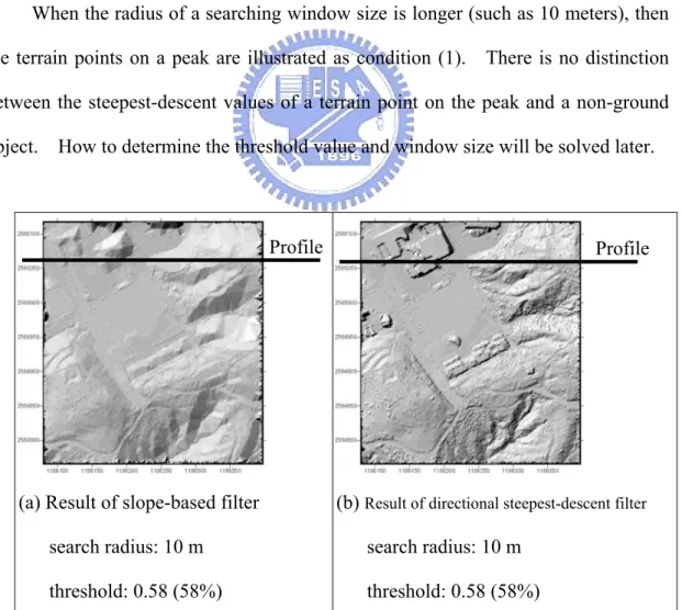
Figure 3.10 and 3.11 show the difference between the slope-based filter and directional steepest-descent filter. The filtering parameters were set at the same values: the search radius as 10 m and the threshold as gradient 0.58 (30° in degree). The slope-based filter removes terrain discontinuities. On the other hand, directional steepest-descent filter preserves terrain features in sloped terrain. However, using a small search radius leads to points on large buildings remaining in both filters.

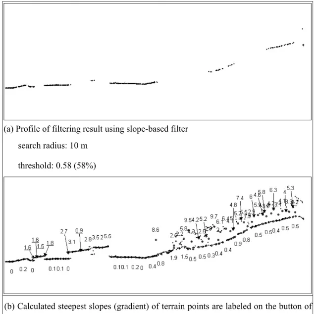
In Figure 3.11, the profile is delineated along the positions as indicated by a solid line on Figure 3.10 showing the elevations and the calculated steepest slopes (equation 3.2) are labeled on the top of the profile. The steepest slopes of terrain points vary from 0.01 to 0.79 on the flat region and vary from 0.23 to 1.91 on relief region respectively. The steepest slopes of non-terrain points vary from 0.73 to 9.05 on the flat region and vary from 1.9 to 9.7 on relief region. The fact that the steepest

slopes for terrain points and non-terrain points could not be accurately classified. On the other hand, the directional steepest descents tan(α) of terrain points vary from 0.01 to 0.5 on the flat region and vary from 0.01 to 0.5 on relief region. The directional steepest descents of non-terrain points vary from 0.25 to 5.92 on the flat region and vary from 0.82 to 9.73 on relief region in Figure 3.11(d).

Directional steepest descent is appropriate for filtering ground objects of smaller sizes. That is, the parameter for the size of a searching window should be small. In order to preserve the terrain points in sloped terrain, the window sizes need to be restricted (Vosselman, 2000). However, a small window size leads to points on large buildings remaining.

When the radius of a searching window size is longer (such as 10 meters), then the terrain points on a peak are illustrated as condition (1). There is no distinction between the steepest-descent values of a terrain point on the peak and a non-ground object. How to determine the threshold value and window size will be solved later.

(a) Result of slope-based filter search radius: 10 m

threshold: 0.58 (58%)

(b) Result of directional steepest-descent filter

search radius: 10 m threshold: 0.58 (58%)

Figure 3.10. Comparison between slope-based and directional steepest-descent filter.

(a) Profile of filtering result using slope-based filter search radius: 10 m

threshold: 0.58 (58%)

(b) Calculated steepest slopes (gradient) of terrain points are labeled on the button of the profile and of non-terrain points are labeled on the top of the profile.

Figure 3.11. Comparison of profile between slope-based and directional steepest-descent filter.

(c) Profile of filtering result using directional steepest descent filter search radius: 10 m

threshold: 0.58 (58%)

(d) Calculated directional steepest descents of terrain points are labeled on the button of the profile and of non-terrain points are labeled on the top of the profile.

Figure 3.11. Comparison of profile between slope-based and directional steepest-descent filter.

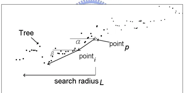
3.4 Adaptive directional steepest-descent filter

In order to filter a large ground object, a searching window must be large enough to completely cover the object. When the searching window size is large,

the background terrain may include complex features. One approach to adaptive thresholding is to subtract background slope from the calculated steepest slope and to perform thresholding as uniform slope result. If the slope value of a given point is much larger than its local background slope, we may classify it as a non-terrain point.

Taking p as a center, point i is found in the direction D and the steepest decent αis obtained. Restarting the process by taking i as a center, and along the azimuth

D within L radial distance, searching for the steepest descent again, the steepest

descentβis obtained (Figure 3.12). If β is positive gradient, then the original steepest descent γ is revised by subtracting β from α , γ = α – β . Thereby, the goal of removing the background slopes is achieved.

Figure 3.12. The steepest-descent is revised by removing the background slopes.

3.5 Adaptive directional elevation-difference filter

The choice of proper window size may be problematic. It is difficult to detect all non-ground objects of various sizes using a fixed window size. For example, in order to remove the measurements of large non-ground objects such as buildings, a larger window size is needed. However, a larger window size may cover complex

terrain or cross a mountain ridge. In this research, for the adoption of a large window size, a different method — directional elevation-difference filter — was developed, as shown in Figure 3.13. First, an initial search radius is used in direction

D to search for a lowest point among the neighbors. Then the search radius is

reduced by one meter, so that the lowest point in each research radius is gradually calculated and selected. The selected lowest points constitute Set G, as illustrated in

Figure 3.13, G1 to G6. The lowest point G1 is found with search radius of L1, and Gk

is found with new search radius of Lk, and so forth. Subsequently, elevation

differences among the sequential lists of Set G are calculated in order, using the

formula dhZD[k] = ZG[k] － ZG[k+1], where k stands for the kth time of reducing the

research radius, and dh(k) constitutes the set dG of elevation differences. In the set dG of elevation differences, the steepest descent δ (maximum value) of elevation difference is therefore selected. Once the calculation in direction D is completed, we can start calculating theδvalue in the next direction. Theδvalues in the four directions are calculated separately, and the minimum will be selected as

{

}

min δ δ δ δ

λ = . Ifλ is lower than the predetermined threshold dhTh,

then this point will be classified as an object point.

Figure 3.13. Finding the lowest point progressively.

search radius is reduced, and G2 (G2=G1 in this case) is found with search radius of L2,

and so forth.

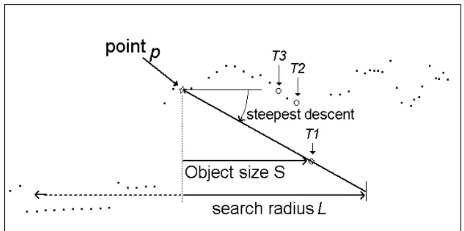
3.6 Determination of search radius

The value of the search radius is a parameter. In this paper, it was proposed that the best search radius for each object point of terrain surface could be calculated automatically. The method of calculation is as follows. First, a larger fixed value is selected as the initial search radius in direction D to search for the lowest spot height among neighboring points. The search radius is then successively reduced, just as with the directional elevation-difference filter described above. The lowest points within each radius are selected and constitute set G. Then the elevation differences among each spot height in set G are calculated, which constitutes the

elevation differences set dG. An elevation difference threshold slopeTh is

predetermined. If the elevation differences (negative value) in the sequential list dG

are smaller than slopeTh, these points are identified as relief spots (less smaller

negative value indicates larger relief). Accordingly, the points in set G are further selected and constitute set T. In set T, the steepest descent between the relief points

and the center p are calculated: Slopek =

2 ] [ 2 ] [ ] [ ) ( ) ( _{p T k p T k} k T p y y x x z z − + − − (the

calculation of slopes between relief points and the center p). The steepest descent is

therefore found, as illustrated in Figure 3.14, point T1. In Figure 3.14, the points in

set T constitute the profile, where the line of sight from point p to T1 is the steepest

descent. The horizontal distance from p to T1 determines the best search radius for

Figure 3.14. Taking p as a center, relief spots are further selected and constitute set T.

3.7 Filtering by multiple filtering procedures

There are two kinds of errors that can be made in quantitative assessment. A Type I error misclassifies bare-Earth points as object points, meaning details of terrain features are lost. Type II errors misclassify object points as bare-Earth points. Since Type II errors will lead to worse results than Type I error in the application of DTM recovering, most filtering tasks tend to produce many more Type I errors than Type II errors (Sithole and Vosselman, 2004). This paper applies the opposite strategy, emphasizing the reduction of Type I errors because Type II errors are easier to fix by multiple filtering procedures.

The procedures of multiple filtering include three stages. In the large objects removal stage (1), an adaptive elevation-difference filter is used to remove large non-ground objects such as buildings. In the medium object removal stage (2), an adaptive steepest-descent filter removes medium non-ground objects such as dense trees. In the final filtering stage (3), a directional steepest-descent filter removes small non-ground objects such as cars and single trees (Figure 3.15).

Figure 3.15. Flowchart of the multiple filtering algorithm. Load raw LIDAR data

(Single return)

Search radius determination

Calculate the elevation differences iteratively

Find the relief points according to the elevation differences Calculate the slope from center point to the relief points Determinate the search radius

Large objects removal by adaptive elevation-difference filtering

Decrease the search radius gradually

Calculate the elevation difference between adjacent points Obtain the minimum elevation-difference for four directions Remove non-terrain points according to the threshold

Medium objects removal by

Adaptive directional steepest-descent filter

Calculate slopes and find the steepest descent at each point Revise the steepest-descent by removing the background slopes Obtain the minimum steepest-descent for four directions Remove non-terrain points according to the threshold

Small objects removal by Directional steepest-descent filter

Reduce the search radius to 3 meters

Obtain the minimum steepest slope for four directions Remove non-terrain points according to the threshold

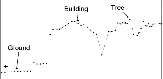
Figure 3.16 delineates a profile with gentle relief that crosses a building and trees. The elevation-difference values are derived along this profile and shown in Figure 3.17. Figure 3.18 shows the steepest-descent values along this profile. Figure 3.17 and 3.18 shows the same phenomenon: these two filters were effective in reducing background nonuniformity.

The values are obtained by subtracting a locally nonuniform background value from the original data and then are suitable to perform a fixed threshold procedure. Before the filtering processes, the point clouds were preprocessed to remove outliers such as birds and low flying aircrafts first. Because high outliers are so far elevated above neighboring points, the filtering process can remove such extreme data easily.

In urban areas, some LIDAR data may contain a few extreme low outliers. These negative blunders are often happened as individual points. When a shaded-relief map was derived, low outliers can be found easily as conical pits. Therefore, extreme low points can be filtered by interactive editing.

Figure 3.17. The elevation-differences values of the sample profile.

Figure 3.18. The steepest-descent values of the sample profile.

3.8 Algorithm implementation

Some algorithms such as morphological operators require the data to be in a grid structure. Interpolating the raw data to a grid causes the height differences in the interpolated data reduced. This research worked with original, irregularly point data.

Determination of search radius

1. Take an initial size of search window L1.

3. Decrease the size of window gradually, and calculate the lowest points as set G. 4. Within set G, calculate elevation differences between two adjacent points iteratively,

which constitutes set dG.

5. Analyze set dG and set G. If the elevation difference between two adjacent points

is smaller than the relief threshold slopeTh (negative of the gradient), then it is

categorized into set T.

6. Within set T, calculate the slope from the center to each point as set SP, and find the steepest descent point U.

7. The size of this object point RD is determined by the distance between point U and

center point p..

8. Go back to step 2. Recalculate the values in the next direction and analyze RD+180.

9. The revised size of initial search radius R on center point p is determined by the

maximum of RD in four directions.

Adaptive directional steepest-descent filter

1. Calculate the initial search radius R by the algorithm described above. 2. In azimuth D, within the R, load raw data of airborne LIDAR.

3. Calculate slope set SP.

4.Within SP, find the steepest descent α at point s.

5. Use site s as the center with a radius of R, obtaining the background steepest descent β.

6. If α and β are negative values at the same time, then subtract the background slopeβ from α : γ = α – β.

7. Go back to step 2. Calculateγ in the next azimuth, γD+180.

8. The minimum Min_γ is selected among γD in the four directions.

non-ground object.

Adaptive directional elevation-difference filter

2.

3.

constitute set G.

4. Within set G, calculate the elevation difference between each two adjacent points, which constitute set dG.

5. Within set dG, find the steepest dh.

6. Go back to step 2. Calculate the values in the next direction, and analyze steepest dhD+180

7. Obtain the minimum Min_dh among four steepest dhD

8. If Min_dh < dhTh, then this point is identified as a ground point; if not, as a

non-ground objects

3.9 Test datasets

In this study, the developed filters were tested on two LIDAR datasets: an urban area and an area of rugged terrain with dense vegetation. The test dataset for urban area is downloaded from the website of ISPRS Commission III, WG III/3 (http://www.commission3.isprs.org/wg3/). The Csiter1_orig.txt and Csiter2_orig.txt are adopted for this study because of the complexity of feature contents. The features of urban test site are steep slopes, mixture of vegetation and buildings on hillside. The point spacing of laser data is around 1.0 – 1.5 meter. The reference datasets include six samples, namely sample 11, sample 12, sample 21, sample 22,

sample 23, and sample 24. The dataset is described in detail in Sithole and Vosselman (2004).

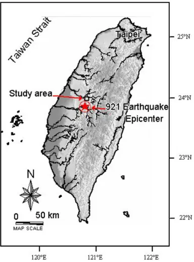
High-relief test site

The high-relief test site is located in central Taiwan. The area is the Jeou-Fen-Er-Shan, a hilly area located in the damaged region of central Taiwan (Figure 3.19). The Chi-Chi earthquake caused a large-scale landslide (1100 m by 1910 m) in this area. The test site is 3 km by 3 km and the elevation ranges from

420 to 1100 m; the slope varies between 0 degree and 70.3 degrees. The 75th

percentile of the slope is 35.8 degrees, and the average is 26.6 degrees, as given in Table 3.1. Figure 3.20 reveals that the study area is in steep terrain and 70% of the slope is greater than 20 degrees. Land-cover types in the study area are dense woods, tea plants, orchard, low grass and sliding rock.

Two datasets were collected in the high-relief test area. The first dataset was collected using an Optech ALTM 2033 system between March 20 and April 3, 2002. The flying height was at a median altitude of 1100 m above ground level. The second dataset was obtained using an LH ALS 40 between April 10 and April 16, 2002, with flying height of 1800 m above ground level. Both datasets were acquired during leaf-on conditions. The H = 1100 m (ALTM 2033) was intended to collect spatially dense (1-m nominal post spacing) LIDAR data, while the mission of the H = 1800 m (ALS 40) was to collect data over a wider area. Table 3.2 compares the parameters of both sets. It shows that the H = 1100 m data involved narrower FOV (30°) than the H = 1800 m data (40°), and that the H = 1100 m was obtained at a higher laser data rate (33 kHz) than the H = 1800 m (25 kHz). Flight directions for both datasets were North-South, oriented parallel to the hills. There are three strips in the H = 1800 m data set, and ten parallel strips for the H = 1100 m data set. The

H = 1100 m data contains an extra East-West flight strip across the study area.

Table 3.1 Statistics of terrain slopes of test site

Statistics Slope (in degree)

Average 26.64 Median 26.59 Std. Deviation 13.03 Minimum 0.01 Maximum 70.38 25th percentile 17.55 75th percentile 35.77

Figure 3.19. High-relief site is located in central Taiwan affected by the Chi-Chi Earthquake. 12% 19% 29% 25 % 12% 3% 1% 0 10 20 30 40 50 60 70 Slope (degrees) 0% 5% 10% 15% 20% 25% 30% 35% P er cent of t ot al ( % )

Table 3.2 LIDAR collection parameters of high relief site

Parameters Altitude H = 1100 m Altitude H = 1800 m

Instrument Optech ALTM 2033 LH ALS 40

Max. terrain height 1154 m 1154 m

Min. terrain height 396 m 396 m

Airplane speed 150 knots (77.17 m/s) 150 knots (77.17 m/s)

Flying altitude (above ground) 900 – 1500 m 1200 – 2200 m

Flight line spacing 400 m 500 m

Pulse rate 33 kHz 25 kHz

Scan rate 38 Hz 27 Hz

Field of view 30° 40°

Swath width 482 – 804 m 870 – 1600 m

Point spacing 1 – 2 m 2 – 3 m

Reference Data of High-relief Area

Data from 906 ground checkpoints, obtained in seven areas with different land-cover, were collected to assess the accuracy of the LIDAR measurement. The measurement incorporates Real-Time-Kinematics (RTK) GPS and the total station technique. The horizontal accuracy of reference data was verified to be about 0.018 m and vertical accuracy 0.020 m, in terms of RMSE. Both the coordinate system of ground checkpoints and the control coordinate system with laser scanning coincided with the same World Geodetic System 1984 (WGS 84) coordinates. Table 3.3 presents the seven evaluation sites:

(1) Pavement area used to assess accuracy on open terrain.

(2) Occlusion path used to assess the accuracy of the occlusion area.

(3) Landslide rock area with homogeneous slopes, with emphasis on the accuracy of the steeper terrain.

(4) Wet soil, covering soft piling and wet soil, with emphasis on the accuracy of wet environment.

(5) Orchard, where only H = 1100 m dataset is available. (6) Tea farm A with 22 degrees average slope.

(7) Tea farm B with 14 degrees average slop.

This test site does not include built-up areas. Figure 3.21 shows the distribution of the surveyed 906 ground checkpoints. Figure 3.22 depicts field and aerial photographs of these evaluation sites.

Table 3.3 Land-cover classes and their descriptions

Class Descriptions

Pavement 9° slopes

Open and flat path

Wet soil 8° slopes

Piling wet soil

Open fields

Occlusion path 8° slopes

High trees on both sides of the 5-m-width path

Landslide rock 25° slopes

Homogeneous steep slope

Open fields

Orchard 9° slopes

Low trees (< 3 meters)

Tea farm A 22° slopes

(a) Pavement

(b) Occlusion path

(c) Landslide rock

(d) Wet soil

(e) Orchard

(f) Tea farm A