Two-Dimensional Adaptive Array Beamforming
With Multiple Beam Constraints Using a Generalized
Sidelobe Canceller
Ju-Hong Lee and Yung-Han Lee
Abstract—This paper deals with the problem of two-dimensional (2-D) adaptive array beamforming with multiple beam constraints (MBC) using a generalized sidelobe canceller (GSC). We present a method for the construction of signal blocking matrix required by the 2-D GSC. The resulting 2-D adaptive beamformer can pro-vide almost the same performance as conventional 2-D adaptive beamformers based on a linearly constrained minimum variance (LCMV) criterion. The effectiveness of the proposed GSC is that the construction of the required signal blocking matrix requires only the computation of a few entries from analytical formulas. In comparison with conventional methods, the proposed technique gets rid of the computational complexity due to the eigendecom-position required for finding the 2-D signal blocking matrix. For dealing with the performance degradation due to coherent inter-ference, we present a 2-D weighted spatial smoothing scheme to ef-fectively alleviate the coherent jamming effect. Several simulation examples are provided for illustration and comparison.
Index Terms—Adaptive beamforming, generalized sidelobe can-celler, multiple beam constraint.
I. INTRODUCTION
R
ESEARCH regarding the design and analysis of adaptive array beamformers is widely focused on the situations of using an array with one-dimensional (1-D) scenario. In this case, the signal sources and the array elements are assumed to be coplanar. However, in many practical applications, there may exist different signals impinging on a 1-D array with different directions, but these signals possess the same angle with respect to the broadside of the 1-D array. However, a 1-D array can only distinguish the azimuth angle or the elevation angle in the ab-sence of a number of interfering signals. Moreover, it is usually impossible to simply extend the principles and techniques of the 1-D case to deal with the mentioned problem. In these circum-stances, we must resort to the use of adaptive beamforming with a two-dimensional (2-D) array scenario.Adaptive beamforming using a generalized sidelobe canceller (GSC) has been widely considered due to its effectiveness and simplicity for achieving multiple linearly constrained beam-forming [1], [2] and partially adaptive beambeam-forming [3]–[6].
Manuscript received June 23, 2004; revised November 10, 2004. This work was supported by the National Science Council under Grant NSC92-2213-E002-033. The associate editor coordinating the review of this manuscript and approving it for publication was Dr. Fulvio Gini.
The authors are with the Department of Electrical Engineering, National Taiwan University, Taipei, 10617, Taiwan, R.O.C. (e-mail: [email protected]).
Digital Object Identifier 10.1109/TSP.2005.853155
Several other advantages of using a GSC-based 1-D adap-tive beamformer over using conventional linearly constrained minimum variance (LCMV) 1-D adaptive beamformers are as follows. 1) The GSC-based adaptive beamformer is easily generalized to deal with main lobe derivative constraints of any order and combined temporal/spatial constraints [1]. 2) The GSC-based adaptive beamformer uses an unconstrained rather than a constrained algorithm to adapt the weights. It is able to adapt much faster [1]. 3) The GSC-based adaptive beamformer is less sensitive to coefficient quantization effects since the dynamic range of the signals in the adaptive portion of the beamformer is compressed [1]. 4) The GSC-based adaptive beamformer is a particularly suitable structure to use for studying the effect of random element amplitude and phase error effects on linearly constrained adaptive beamformers [19], [20]. However, there is very little work concerning adap-tive beamforming based on GSC structure using a 2-D array. Recently, Salem et al. [7] presented the direct design of a GSC using a 2-D array to carry out 2-D adaptive beamforming with a main-beam constraint. Nevertheless, the 2-D blocking matrix of the designed GSC is constructed from the formula , where denotes the normalized elevation-azimuth steering vector of the desired signal, the superscript is constructed from the conjugate transpose, and is constructed from the zero vector. Accordingly, the procedure for finding the required 2-D blocking matrix is the direct extension of the 1-D case. This leads to the drawback that the computation complexity increases rapidly as the dimension of the 2-D array increases.
For many practical applications, such as satellite communi-cations [8], an antenna array is required to possess the beam-forming capability that receives more than one signal with spec-ified gain constraints while suppressing all jammers. This goal can be achieved using an antenna array with a multiple-beam pattern [8], [9]. In the case of satellite communications using adaptive beamforming, short convergence time would be re-quired for some applications like a target application. Yu [9] pro-poses an adaptive algorithm that finds an adaptive weight vector that is close to a desired quiescent beam pattern under a unit norm constraint on the weight. However, a sophisticated pro-cedure is required to solve the resulting nonlinear optimization problem. To tackle this problem, Lee et al. [10] develop a tech-nique based on Frost’s algorithm [11] to provide adaptive beam-forming with multiple-beam constraints (MBCs). However, this technique can only deal with the 1-D case.
In this paper, we present a technique to construct a GSC-based 2-D adaptive beamformer that possesses the capability
to provide MBC as well as coherent jamming suppression. To achieve the first goal of using a GSC, we develop a mathemat-ical formula for the construction of the 2-D signal blocking ma-trix . The formula provides an analytical solution that finds the entries of the required without the need for the compu-tational complexity required by the conventional approach like [7]. Then, using the 2-D signal blocking matrix , we formu-late the 2-D beamforming problem as finding such a quiescent weight matrix that the 2-D array output power is minimized subject to a set of a specified MBC. It is shown that an ana-lytical solution for the resulting minimization problem can be easily obtained to satisfy the goal of providing MBC as well as jamming suppression. To achieve the second goal of effec-tively curing the problem due to the coherence between the de-sired signals and interferers, a 2-D weighted spatial smoothing scheme is presented. Several simulation examples are given to show the effectiveness of the proposed technique.
This paper is organized as follows. In Section II, we briefly describe the theory of 2-D adaptive beamforming using a GSC. Section III presents the technique for constructing a GSC-based 2-D adaptive beamformer with MBC. We introduce a 2-D weighted spatial smoothing scheme in Section IV. Several simulation examples are provided in Section V for illustration. We finally conclude the paper in Section VI.
II. TWO-DIMENSIONALADAPTIVEARRAYBEAMFORMING
USING AGSC
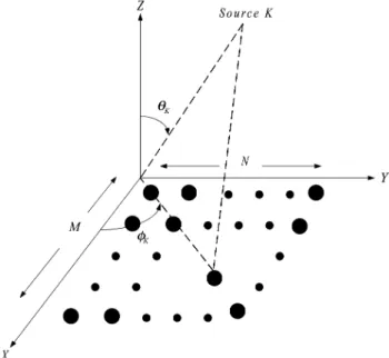
As shown in Fig. 1, a 2-D uniform planar array (UPA) with size has sensors located on the 2-D X-Y plane at the
positions for and
, where is the smallest signal wavelength of the signals with specified gain arrangements. Assume that the array phase center is set to the th sensor located at the
position . Let the signal impinging
on the 2-D array from the evaluation angle and azimuth angle yield a unit magnitude response and a phase response given
by at the array sensor located
at , where , and
. narrowband and far-field signals are impinging on the 2-D UPA from distinct direction
angles for . Hence, the data received by
the th sensor can be written as
(1) where denotes the complex waveform of the th signal source, and signifies the spatially white sensor noise in-dependent of . For simplicity, assume that the first signal sources are the desired signals with specified gain arrangements
and direction angles for , whereas the
other signals are interferers. From (1), we can express the data matrix received by the 2-D UPA as follows:
(2)
Fig. 1. Two-dimensional uniform planar array.
where
,
, and denotes the noise matrix received by the 2-D UPA. The superscript represents the transpose operation. In vector form, we rewrite (2) as follows:
vec
(3) Based on the property of the Kronecker product [12]
vec vec , where are
matrices with appropriate sizes, (3) can be written as follows:
vec vec
(4) where the response vector of the th signal source
, the response matrix of the signal sources , and the signal
source vector . As a result, we
have the correlation matrix of vec given by
vec vec (5)
where denotes the correlation matrix of
the signal sources, denotes the noise power, and denotes the identity matrix. Equation (5) reveals that exhibits a block Toeplitz structure if the distinct signal sources are uncorrelated.
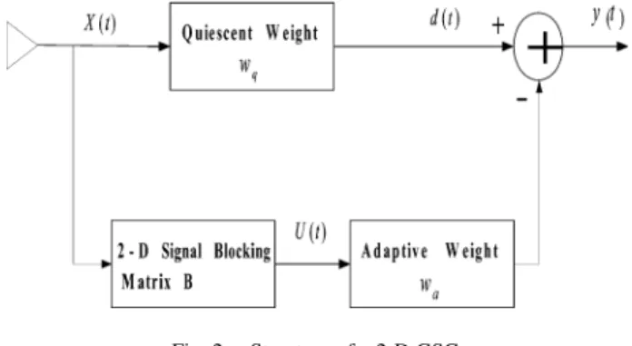
Consider the GSC structure shown by Fig. 2. It has been widely recognized that 1-D adaptive array beamforming using a GSC possesses the advantages of easy implementation and the assessment of the performance degradation due to steering or gain errors in array sensors. For the 2-D case with MBC, the output signal of the upper branch is given by
Fig. 2. Structure of a 2-D GSC.
is the quiescent component of the overall weight vector of the GSC and used to realize the constrained weight subspace, which is spanned by the column vectors of the constraint ma-trix . Hence, the design of is asked to satisfy a set of linear constraints given by
(6)
where denotes the
con-straint matrix with size , and is
a gain vector containing the specified gain arrangements for the desired signal sources. Accordingly, can be found as follows:
(7) The sidelobe canceling branch is used for the realization of the unconstrained weight subspace that is complementarily or-thogonal to the column space of the constraint matrix . The 2-D signal blocking matrix is employed to block the de-sired signals from the received data vector . It follows that
with size must be orthogonal
to , i.e., . The signal at the array output is given
by . In this context, the adaptive
weight is the optimal solution for the unconstrained mini-mization problem:
Minimize (8)
This leads to the fact that is given by
(9) The overall weight vector for the 2-D GSC-based adaptive beamformer becomes
(10)
III. CONSTRUCTION OF2-D SIGNALBLOCKINGMATRIX
From (10), we note that the construction of the required 2-D signal blocking matrix must satisfy the condition of
. According to existing techniques like [7], the 2-D blocking
matrix with size is directly
com-puted from the formula . This leads to the need for complicated computations including the singular value decom-position (SVD) of , and hence, the required computational
burden is [13]. In the following, we
present a technique to efficiently construct the 2-D blocking ma-trix without the above complicated computations.
From (4), we note that the response vector of the th
signal source with given by
and given by .
Let and . Then, we have
, ,
and .
Accordingly, the constraint matrix can be expressed as .
The condition of indicates that
, . We express the product as
follows:
8 (11)
where8 and are given by
8
and (12)
respectively.8 and are two algebraic expressions used to represent that the condition of must be
sat-isfied at and , . Moreover,
and are two vectors used to stand for the remaining parts of after we extract the roots
at and , and are given by
(13) where
and
(14)
with ,
respectively. In order to make the equality in the dimen-sion for the vectors shown in (11), zero en-tries must be appended to the vector since
if . Hence, both
and have size . In
contrast, zero entries must be appended to the
vector since if
. Thus, both and have size
. Since
, we have the th
entry of the vector , which is given
by
for if and
if . Based on the results of (11), (12), and (15), we can compare each entry corresponding to the both sides of (11)
to find the , , and
if or if , which
required to construct the 2-D signal blocking matrix with size
if and if .
For illustration, we present the formulas to compute the entries
of as follows. For and , (12) becomes
8 , and9 . According to
(15), we can easily find equal to
for for for otherwise for (16) for for for for otherwise for (17) for for for for otherwise for (18) for for for otherwise for (19)
Following the similar procedure, we can also find the entries of the resulting 2-D signal blocking matrix for the case of and , which is given as (20)–(22), shown at the bottom of the page. As far as the general case of , i.e., a 2-D rectangular array, we present the resulting in the case of and for illustration as follows. First, the
response vector becomes with
and . Therefore,
. For , (12) becomes 8 and
. According to (15), we can easily find equal to for for for otherwise for (23) for for for for otherwise for (24) for for for for otherwise for (25) for for for and for otherwise for (20) for for for for for and otherwise for (21) for for for for for otherwise for (22)
To find the entries , , , we have to utilize the formula given by (11) and compare each entry corresponding to the both sides of (11). The resulting 2-D signal blocking matrix for the case of is given as in (26), shown at the bottom of the page. Following a similar procedure, we can also find the resulting 2-D signal blocking matrix for the case of given as in (27), shown at the bottom of the page.
From the constructed 2-D signal blocking matrix , we
ob-serve that it has size of ,
where denotes the maximum of and , and
min the minimum of and . Therefore, the pro-posed 2-D signal blocking matrix requires significantly fewer entries as compared with the one proposed by Salem et al. [7] with size . This reveals that the proposed GSC-based 2-D array beamformer can provide satisfactory per-formance by requiring only
instead of adaptive weights.
Finally, we evaluate the computational complexity in terms of complex multiplications (CM) required for constructing the 2-D signal blocking matrix using the proposed method. Here, we describe the number of the CMs required for the construction of the proposed 2-D signal blocking matrix for desired signals as follows:
1) For , we follow the formulas of (12), which become
8 and8 , respectively.
Hence, computing the coefficients by (15) requires no CM at all. 2) For , the formulas of (12) become8
and9 ,
respec-tively. Computing the coefficients by (15) requires the CM for obtaining and , i.e., the number of CM required
is . 3) For , the formulas of
(12) become8 and
9 , respectively.
Com-puting the coefficients by (15) requires the CM for obtaining
, , , , and , ,
, , i.e., the number of CM required is . Following the similar procedure described above, we can derive the gen-eral formula for calculating the number of CM required for any value of as follows:
(28)
where represents the number of
-el-ement combinations of objects. Clearly, is significantly less than that required by using the conventional method [7].
(26)
Fig. 3. Subarray grouping for a 2-D uniform planar array.
IV. TWO-DIMENSIONALWEIGHTEDSPATIAL
SMOOTHINGSCHEME
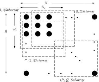
In the presence of coherence between the desired signals and interferers, the performance of a 2-D array beamformer deteri-orates due to the signal cancellation phenomenon. According to the approach proposed by [14], we first briefly describe the 2-D spatial smoothing (2-D SS) scheme for a 2-D uniform planar array (UPA). For simplicity, we use a simple example for demonstration. Let the 2-D UPA be grouped into overlapping subarrays of size , as shown in Fig. 3. Assume that represents the input vector of the th subarray, which consists of the th to the th rows and the th to the th columns of the 2-D UPA. The autocorrelation matrix of the th subarray is then given by . Following the 2-D SS scheme of [14], we obtain the 2-D spatially smoothed autocorrelation
matrix by taking . In order
to successfully decorrelate coherent signals, the condition must be held. Then, is used instead of , which is shown by (5) to perform 2-D adaptive beamforming. However, similar to the 1-D case, the effectiveness of the conventional 2-D SS is limited because the effective aperture
size is reduced due to and . Moreover,
the 2-D spatially smoothed autocorrelation matrix cannot possess the block Toeplitz property from the simple averaging
on .
To tackle the drawbacks of using conventional 1-D spa-tial smoothing scheme of [15], Takao et al. [16] presented a so-called weighted spatial smoothing (WSS) scheme, which adapts the variable weights instead of uniform weighting to obtain a 1-D spatially smoothed autocorrelation matrix. The variable weights are found through a Toeplitzization algorithm that makes the resultant spatially smoothed matrix Toeplitz. Recently, this technique of [16] was extended by Indukumar et
al. [17] to solve the coherent problem when dealing with
broad-band signals. In the literature, there are practically no papers considering an appropriate WSS scheme that deals with the case of using a 2-D planar array. In the following, we introduce a 2-D WSS scheme to tackle the coherence between signal
TABLE I
CONCATENATION OFEQUATIONS ANDRELATIONS FOR THE2-D WSS SCHEME
sources and to ensure that the obtained spatially smoothed autocorrelation matrix is block Toeplitz.
Let the sampled version of the 2-D autocorrelation matrix be , which is obtained by taking data snapshots. We express as follows:
..
. ... ... ... (29)
where denotes the cross-correlation matrix of the data vectors received by the th and th column subarrays, re-spectively. Then, a 2-D block-Toeplitz approximation method (2-D BTAM) is presented to construct an block Toeplitz matrix as follows:
..
. ... ... ...
(30)
where
(31) are all Toeplitz matrices with size , and denotes the Toeplitzization operation performed on matrix and is given by (32) where
(33) and represents the th entry of . The subscript “bt” in (30) indicates that the obtained matrix possesses the block Toeplitz property. We note that is the solution of the following minimization problem:
where represents the set of Toeplitz matrices with size , and denotes the Frobenius norm of the matrix [18] Moreover, (30) reveals that the constructed matrix is also Hermitian.
Based on the above 2-D SS and 2-D BTAM schemes, we in-troduce a 2-D WSS as follows. First, we reorder the 2-D sub-arrays. Let the th 2-D subarray be denoted by the th 2-D subarray according to the relationship of . Then, we perform the 2-D SS with imposed weights on the 2-D UPA to obtain the 2-D spatially smoothed autocorrelation ma-trix as follows:
(35) where are the real weights to be chosen subject to for taking the average from the autocorre-lation matrix of the th 2-D subarray. Then, the above 2-D
BTAM is performed on to produce . We
define a parameter to represent the measure of deviation of from as follows:
(36)
where and denote the th
el-ements of and , respectively. In matrix form, we rewrite (36) as follows:
(37)
where denotes the weighting vector
and is given by
Re (38)
where the vector has the th entry
given by
(39)
where and represent the
th elements of and , respectively.
The optimal weights can be found by performing the following optimization problem:
Minimize
Subject to (40)
where the vector . The optimal
solu-tion for (40) is given by
(41) Table I lists the concatenation of the equations and the relations for the 2-D WSS scheme. Substituting into (35) yields a spa-tially smoothed autocorrelation matrix that is very close to a
(a)
(b)
(c)
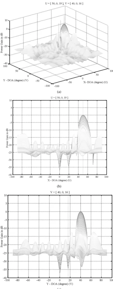
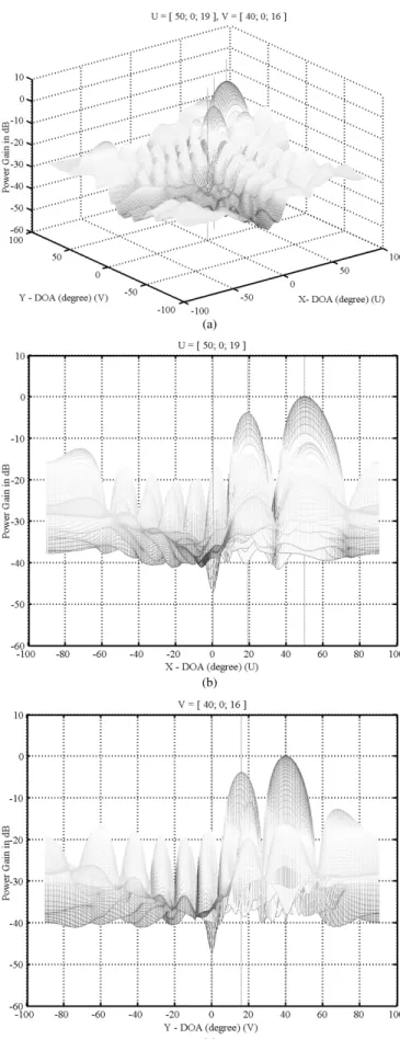
Fig. 4. (a) Two-dimensional array beam pattern without coherence for Example 1. (b) Beam pattern in theU direction without coherence for Example 1. (c) Beam pattern in theV direction without coherence for Example 1.
block Toeplitz structure. Due to spatial smoothing, the effective 2-D aperture size becomes . We construct a 2-D signal
(a)
(ab)
(c)
Fig. 5. (a) Two-dimensional array beam pattern with coherence for Example 1. (b) Beam pattern in theU direction with coherence for Example 1. (c) Beam pattern in theV direction with coherence for Example 1.
blocking matrix using the technique presented in Section III with 2-D array size instead of , and we
com-(a)
(b)
(c)
Fig. 6. (a) Two-dimensional array beam pattern after using 2-D SS for Example 1. (b) Beam pattern in theU direction after using 2-D SS for Example 1. (c) Beam pattern in theV direction after using 2-D SS for Example 1.
pute the overall weight vector from (10) based on the obtained
(a)
(b)
(c)
Fig. 7. (a) Two-dimensional array beam pattern after using 2-D WSS for Example 1. (b) Beam pattern in theU direction after using 2-D WSS for Example 1. (c) Beam pattern in the V direction after using 2-D WSS for Example 1.
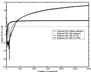
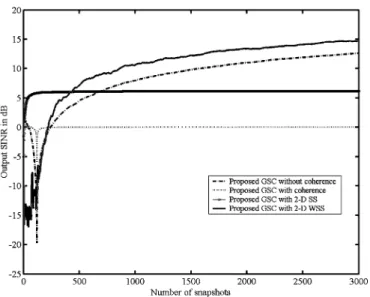
Fig. 8. Output SINR versus number of snapshots for Example 1. TABLE II
OUTPUTSINRS(INDECIBELS)OFUSINGDIFFERENTMETHODS FOREXAMPLE1
V. COMPUTERSIMULATIONEXAMPLES
In this section, several simulation examples performed on a Pentium IV PC using the MATLAB programming language are presented for illustration, confirming the theoretical works. The array used for all simulations is a 2-D UPA with the interelement spacing equal to , where is the smallest wavelength of the desired signals. All signals used for simulations are binary phase shift keying (BPSK) narrowband signals with cosine waveform shape and carrier frequency equal to 1 Hz. The array phase center is set to the (6,6)th sensor. All simulation results pre-sented are obtained by averaging 30 independent runs with in-dependent noise samples for each run. The received noise is spa-tially white noise with variance equal to 1 and zero mean. More-over, in dealing with the case of coherent signal sources, the simulation results using conventional 2-D SS are also presented for comparison. To facilitate the work of plotting array beam patterns, the coordinate system used is instead of
with and ,
re-spectively.
Example 1: This example considers the case of . Three signal sources with signal-to-noise (SNR) all equal to 0 dB are impinging on the array from direction
an-gles , , and
, respectively. Assume that the spec-ified signal is the first signal with and that the others are the jammers. Moreover, the signals with direction angles
(a)
(c)
(c)
Fig. 9. (a) Two-dimensional array beam pattern without coherence for Example 2. (b) Beam pattern in theU direction without coherence for Example 2. (c) Beam pattern in theV direction without coherence for Example 2.
and are coherent.
and are set to 11. The subarray size for performing 2-D SS and 2-D WSS is set to . Accordingly, the
(a)
(b)
(c)
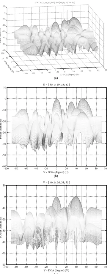
Fig. 10. (a) Two-dimensional array beam pattern with coherence for Example 2. (b) Beam pattern in theU direction with coherence for Example 2. (c) Beam pattern in theV direction with coherence for Example 2.
number of subarrays used is 4. Figs. 4–7 plot the simulation results in terms of the array beam patterns, and Fig. 8 depicts
(a)
(b)
(c)
Fig. 11. (a) Two-dimensional array beam pattern after using 2-D SS for Example 2. (b) Beam pattern in theU direction after using 2-D SS for Example 2. (c) Beam pattern in theV direction after using 2-D SS for Example 2.
the corresponding array output signal-to-interference plus noise ratio (SINR) by utilizing the proposed GSC-based 2-D adaptive beamformer with conventional 2-D SS and with 2-D
(a)
(b)
(c)
Fig. 12. (a) Two-dimensional array beam pattern after using 2-D WSS for Example 2. (b) Beam pattern in theU direction after using 2-D WSS for Example 2. (c) Beam pattern in theV direction after using 2-D WSS for Example 2.
WSS for comparison. The output SINRs obtained by using 30 000 data snapshots for the results of using the 2-D WSS,
Fig. 13. Output SINR versus number of snapshots for Example 2. TABLE III
OUTPUTSINRS(IN DECIBELS) OFUSINGDIFFERENTMETHODS FOREXAMPLE2
the conventional 2-D SS, the result with coherence, and the result without coherence are listed in Table II. Three methods are presented for comparison: the proposed method, the 2-D conventional LCMV method that is a direct extension of the 1-D case [11], and the traditional 2-D GSC of [7]. We observe that the simulation results confirm the validity of the proposed method’s capabilities for 2-D adaptive beamforming. The pro-posed method outperforms the traditional 2-D GSC [7] and the 2-D conventional LCMV method [11] in the main beam case.
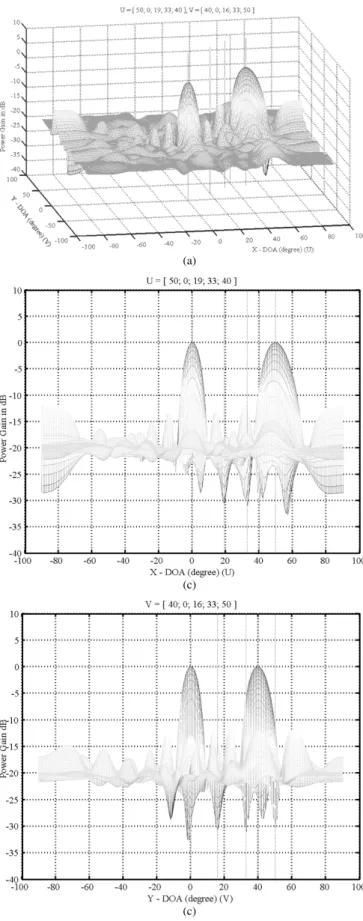
Example 2: This example considers the case of . Five signal sources with SNR all equal to 0 dB are impinging on the
array from direction angels ,
, , , and
, respectively. Assume that the specified signal is the first two signals with , and the others are the jammers. Moreover, the signals with direction angles
and ,
and are coherent, respectively.
and are set to 12. The subarray size for performing 2-D SS and 2-D WSS is set to . Accordingly, the number of subarrays used is 16. Figs. 9–12 plot the simulation results in terms of the array beam patterns, and Fig. 13 depicts the corresponding array output SINR by utilizing the proposed GSC-based 2-D adaptive beamformer with conventional 2-D SS and with 2-D WSS for comparison. The output SINRs ob-tained by using 30 000 data snapshots for the results of using the 2-D WSS, the conventional 2-D SS, the result with coher-ence, and the result without coherence are listed in Table III.
Again, three methods are presented for comparison: the pro-posed method, the 2-D conventional LCMV method that is a direct extension of the 1-D case [11], and the traditional 2-D GSC of [7]. Again, the simulation results confirm the validity of the proposed method’s capabilities for 2-D adaptive beam-forming. The proposed method outperforms the traditional 2-D GSC [7] and the 2-D conventional LCMV method [11] in the MBC case.
VI. CONCLUSION
This paper has presented a method to construct a generalized sidelobe canceller (GSC) for performing 2-D adaptive array beamforming with multiple-beam constraints using a 2-D uni-form planar array. Through the presented analytical uni-formulas, the 2-D signal blocking matrix required by the 2-D GSC can be computed analytically without the need for complicated singular value decomposition. In the case with coherent signal sources, a 2-D weighted spatial smoothing scheme is proposed to effectively decorrelate the coherence between coherent sig-nals, and hence, the performance degradation due to coherence can be alleviated. As compared with the existing 2-D spatial smoothing scheme, which is the most notable method for tackling coherent situation, several simulation examples have confirmed the validity of the theoretical works and shown that the proposed method can provide satisfactory performance.
REFERENCES
[1] L. J. Griffiths and C. W. Jim, “An alternative approach for linearly con-strained adaptive beamforming,” IEEE Trans. Antennas Propag., vol. AP-30, pp. 27–34, Jan. 1982.
[2] K. M. Buckley and L. J. Griffiths, “An adaptive generalized sidelobe canceller with derivative constraints,” IEEE Trans. Antennas Propag., vol. AP-34, pp. 311–319, Mar. 1986.
[3] K. Takao and K. Uchida, “Beamspace partially adaptive antenna,” Proc. Inst. Elect. Eng., H, Microwave Antenna Propag., vol. 136, pp. 439–444, Dec. 1989.
[4] B. D. Van Veen, “Eigenstructure based partially adaptive array design,” IEEE Trans. Antennas Propag., vol. 36, no. 3, pp. 357–362, Mar. 1988. [5] B. D. Van Veen and R. A. Roberts, “Partially adaptive beamformer design via output power minimization,” IEEE Trans. Acoust., Speech, Signal Process., vol. ASSP-35, no. 11, pp. 1524–1532, Nov. 1987. [6] S. -J. Yu and J. -H. Lee, “Design of partially adaptive beamformers based
on information theoretic criteria,” IEEE Trans. Antennas Propag., vol. 42, no. 5, pp. 676–689, May 1994.
[7] I. Salem, A. Hanafy, H. G. Hussein, and A. D. Moufid, “Two-dimen-sional generalized sidelobe canceller (GSC) with partial adaptivity,” in Proc. Eighteenth Nat. Radio Science Conf., Mansoura, Egypt, Mar. 2001, pp. 81–88.
[8] J. T. Mayhan, “Area coverage adaptive nulling from geosynchronous satellites: Phased arrays versus multiple-beam antennas,” IEEE Trans. Antennas Propag., vol. AP-34, pp. 410–419, Mar. 1986.
[9] K. -B. Yu, “Adaptive beamforming for satellite communication with selective earth coverage and jammer nulling capability,” IEEE Trans. Signal Process., vol. 44, no. 12, pp. 3162–3166, Dec. 1996.
[10] J. -H. Lee and T. -F. Hsu, “Adaptive beamforming with multiple-beam constraints in the presence of coherent jammers,” Signal Process., vol. 80, pp. 2475–2480, May 2000.
[11] O. L. Frost, “An algorithm for constrained adaptive array processing,” Proc. IEEE, vol. 60, no. 8, pp. 926–935, Aug. 1972.
[12] A. Graham, Kronectker Products and Matrix Calculus With Applica-tions. New York: Ellis Horwood, 1981.
[13] G. H. Golub and C. F. Van Loan, Matrix Computations, Second ed. Baltimore, MD: Johns Hopkins Univ. Press, 1989.
[14] C.-C. Yeh, J.-H. Lee, and Y.-M. Chen, “Estimating two-dimensional an-gles-of-arrival in coherent source environment,” IEEE Trans. Acoust., Speech, Signal Process., vol. 37, no. 1, pp. 153–155, Jan. 1989.
[15] T. J. Shan and T. Kailath, “Adaptive beamforming for coherent signals and interference,” IEEE Trans. Acoust., Speech, Signal Process., vol. ASSP-33, no. 3, pp. 527–536, Jun. 1985.
[16] K. Takao and N. Kikuma, “An adaptive array utilizing adaptive spatial averaging technique for multipath environment,” IEEE Trans. Antennas Propag., vol. AP-35, no. 12, pp. 1389–1395, Dec. 1987.
[17] K. C. Indukumar and V. U. Reddy, “Decorrelation of broadband signals by Toeplitz-block-Toeplitz structuring,” IEEE Trans. Aerosp. Electron. Syst., vol. 30, no. 3, pp. 685–697, Jul. 1994.
[18] J. A. Cadzow, “Signal enhancement—A composite property mapping algorithm,” IEEE Trans. Acoust., Speech, Signal Process., vol. 36, no. 1, pp. 49–62, Jan. 1988.
[19] C. W. Jim and L. J. Griffiths, “Random Gain and Phase Error Effects in Opyimal Array Structures,” Dept. Elec. Eng., Univ. Colorado, Boulder, CO, Tech. Rep. EE 77-2, 1977.
[20] L. J. Griffiths and C. W. Jim, “A Generalized Sidelobe Canceling Struc-ture for Adaptive Arrays,” Signal Process. Lab., Dept. Elec. Eng., Univ. Colorado, Boulder, CO, Tech. Rep. SPL 78-2, 1978.
Ju-Hong Lee was born in I-Lan, Taiwan, R.O.C.,
on December 7, 1952. He received the B.S. degree from the National Cheng-Kung University, Tainan, Taiwan, in 1975, the M.S. degree from the National Taiwan University (NTU), Taipei, in 1977, and the Ph.D. degree from Rensselaer Polytechnic Institute (RPI), Troy, NY, in 1984, all in electrical engineering.
From September 1980 to July 1984, he was a Re-search Assistant and was involved in reRe-search on mul-tidimensional recursive digital filtering with the De-partment of Electrical, Computer, and Systems Engineering, RPI. From August 1984 to July 1986, he was a Visiting Associate Professor and, in August 1986, became an Associate Professor with the Department of Electrical Engineering, NTU, where, since August 1989, he has been a Professor. He was appointed Visiting Professor with the Department of Computer Science and Electrical Engineering, University of Maryland, Baltimore, during a sabbatical leave in 1996. His current research interests include multidimensional digital signal cessing, image processing, detection and estimation theory, analysis and pro-cessing of joint vibration signals for the diagnosis of cartilage pathology, and adaptive signal processing and its applications in communications.
Dr. Lee received Outstanding Research Awards from the National Science Council (NSC) of Taiwan in 1988, 1989, and from 1991 to 1994, and Distin-guished Research Awards from the NSC from 1998 to 2004.
Yung-Han Lee was born in Taipei, Taiwan, R.O.C.,
on July 11, 1977. He received the B.S. degree in elec-trical engineering from the National Ocean Univer-sity, Keelung, Taiwan, in 1999 and the M.S. degree from the Graduate Institute of Communication En-gineering of National Taiwan University, Taipei, in 2004.
His current research interests include adaptive array signal processing and its applications in wireless communications.