結合禁忌演算法與模擬退火演算法推求三維空間地下水污染源

全文

(1)國. 立. 交. 通. 大. 學. 環境工程研究所碩士論文. 結合禁忌演算法與模擬退火演算法推求三維空間地下水污染源 Combining Tabu Search and Simulated Annealing for Identifying Three-Dimensional Groundwater Contaminant Source. 研究生：張桐樺指導教授：葉弘德教授. 中華民國九十四年六月.

(2) 結合禁忌演算法與模擬退火演算法推求三維空間地下水污染源 Combining Tabu Search and Simulated Annealing for Identifying Three-Dimensional Groundwater Contaminant Source. 研究生：張桐樺. Student: Tung-hua Chang. 指導教授：葉弘德. Advisor: Hund-Der Yeh. 國立交通大學環境工程研究所碩士論文. A Thesis Submitted to Institute of Environmental Engineering College of Engineering National Chiao Tung University In Partial Fulfillment of the Requirements For the Degree of Master of Science In Environmental Engineering June, 2004 Hsinchu, Taiwan. 中華民國九十四年六月 2.

(3) 摘要本研究提出一個方法，融合禁忌演算法與模擬退火演算法的優點，並結合美國地質調查局所研發之三維地下水流與傳輸模擬模式 MODFLOW-GWT，做為污染源鑑定的工具，針對在監測井測得的污染分佈，推求地下水污染源的位置、釋放時間、及釋放濃度。在本研究中，先設定在自由含水層中，一個污染源位置為已知（以下稱實際污染源）且某污染物連續釋放三年，利用 MODFLOW-GWT 模式模擬下游的濃度分布。在模擬時，將此含水層以等厚度分為四層，可算得在已知位置的監測井中，於不同深度時的實際濃度值。其後，在實際污染源周圍，選擇一個區域列為可疑的污染源區域，並將此區域內格網的節點位置，皆視為候選污染源的釋放點，並設定各監測井的深度，要逆推的未知數，為各候選污染源三維空間的位置、釋放濃度、及釋放時間。在進行污染源推求時，利用禁忌演算法及模擬退火演算法不同的演算特性，分別產生一系列污染源位置、污染物釋放時間、及釋放濃度的試誤解，利用禁忌演算法選取候選污染源位置的試誤解，並以模擬退火演算法產生釋放濃度及時間的可能解，隨後用 MODFLOW-GWT 進行污染物的傳輸模擬，得到在各監測井的模擬濃度值。當所得結果滿足所設定的目標函數時，亦即模擬濃度與實際濃度差值的平方和最小時，即表示求得污染源的位置與所釋放污染物的濃度和釋放時間。由數值模擬的結果顯示，即使觀測濃度包含誤差，本研究所發展的方法依然能得到精確的推估結果。此外，本研究由數值模擬結果，提出最佳的監測井個數. I.

(4) 與有效鑑定污染源的準則。. II.

(5) Abstract. An approach, combining the tabu search, simulated annealing, and a three-dimensional groundwater flow and solute transport model (MODFLOW-GWT) is developed to estimate the source information including source location, release concentration, and length of release period.. At the development stage of the. proposed approach, the measured concentrations at sampling points are simulated by MODFLOW-GWT with the assumed release concentration at known source location (hereinafter referred to as real source).. In the source information estimation process,. a suspicious source area covering the real source is delimited at beginning.. Then the. source location is chosen by tabu search from the suspicious source area and a series of trial solutions for release concentration and release period are generated by simulated annealing.. The MODFLOW-GWT is employed with those generated. source information to simulate the plume concentrations at sampling points.. The. source estimation process is terminated when the sum of square error between simulated concentration and measured concentration is minimized.. The proposed. approach gives good estimate results even the measured concentrations contain measurement errors.. In addition, a guideline regarding to the optimal number of. sampling points and the condition for effectively estimating source information is also. III.

(6) concluded in this thesis.. IV.

(7) TABLE OF CONTENTS 摘要.......................................................................................................................................................... I ABSTRACT ......................................................................................................................................... III TABLE OF CONTENTS....................................................................................................................... V LIST OF FIGURES ............................................................................................................................VII NOTATION....................................................................................................................................... VIII CHAPTER 1 INTRODUCTION...........................................................................................................1 1.1 BACKGROUND................................................................................................................................1 1.2 OBJECTIVES...................................................................................................................................2 CHAPTER 2 LITERATURE REVIEW ...............................................................................................4 2.1 SOURCE IDENTIFICATION..............................................................................................................4 2.2 MONITORING WELL DESIGN.........................................................................................................8 CHAPTER 3 METHODOLOGY........................................................................................................12 3.1 GROUNDWATER FLOW AND TRANSPORT ....................................................................................12 3.2 SIMULATED ANNEALING .............................................................................................................13 3.3 TABU SEARCH ..............................................................................................................................15 CHAPTER 4 IDENTIFICATION PROCESS....................................................................................17 CHAPTER 5 EXAMPLES AND RESULTS ......................................................................................21 5.1 NUMERICAL EXAMPLES ..............................................................................................................21 5.2 EIGHT SCENARIOS AND RESULTS................................................................................................22 5.2.1 Scenario 1: Initial guesses for the source information ......................................................24 5.2.2 Scenario 2: Upper bound of the solution domain ..............................................................25 5.2.3 Scenario 3: Measurement error ..........................................................................................27 5.2.4 Scenario 4: Number of sampling points .............................................................................28 5.2.5 Scenario 5: A guideline for effectively estimating source information..............................29 5.2.6 Scenario 6: Guideline verification......................................................................................30 5.2.7 Scenario 7: Depth of source and well allocation................................................................33 5.2.8 Scenario 8: Heterogeneous aquifer ....................................................................................34 CHAPTER 6 CONCLUSIONS ...........................................................................................................37 REFERENCE .......................................................................................................................................39. V.

(8) LIST OF TABLES. Table. 1 The sampling points and the measured concentrations for the homogeneous aquifer when the real source is located at the depth of -9 m..........................44 Table 2 The results of 7 cases designed in the first scenario for studying the effect of initial guesses on source information estimation ...........................................45 Table 3 The results of 6 cases designed in the second scenario for the examination of the solution domain........................................................................................46 Table 4 The results of 3 cases designed in the third scenario for the effect of measurement error on source information estimation ...................................47 Table 5 The results for 5 cases designed in the fourth scenario for the examination of the number of sampling points.......................................................................48 Table 6 The results of 11 cases designed in the fifth scenario to find the guideline for effectively source information estimation .....................................................49 Table 7 The results of 16 cases designed in the sixth scenario to verify the guideline for effectively source information estimation................................................50 Table 8 The measured concentrations used in seventh scenario when real source is located at -3 m, -9m, -15 m, or -21 m ............................................................51 Table 9 The results of 8 cases designed in the seventh scenario for the examination of source depths..................................................................................................52 Table 10 The sampling points and the measured concentrations for a heterogeneous aquifer when the real source is located at the depth of -9 m..........................53 Table 11 The results of 4 cases designed in the eighth scenario for the examination of heterogeneous aquifer ....................................................................................54. VI.

(9) LIST OF FIGURES. Figure 1 Flowchart of tabu search ...............................................................................55 Figure 2 Flowchart of SATS-GWT..............................................................................56 Figure 3 Flowchart of TS process in SATS-GWT .......................................................57 Figure 4 The aquifer system with an area of 1000m by 1000m (not to scale) and the locations of real source S1, eight suspicious source near S1, and well A to well J. .............................................................................................................58. VII.

(10) NOTATION. Kij. ： Hydraulic conductivity. h. ： Hydraulic head. Ss. ： Specific storage. t. ： Time. W. ： Volumetric flux per unit volume. xi. ： The Cartesian coordinates. ε. ： Porosity of the aquifer. C. ： Release concentration. Vi. ： Velocity of groundwater flow. Di. ： Dispersion coefficient. C′. ： Concentration of the source/sink fluid. x’. ： Trial solution. f(x’). ： Objective function value of x’. RD. ： Random number. Xi. ： Grid of current location located in x-coordinate. Xi+1. ： Grid of candidate location located in x-coordinate. r. ： Step length factor. Te. ： Current temperature. PSA. ： Acceptance probability of the trial solution x’. PL. ： Acceptance probability of the candidate location. P. ： Release period. Ci,est. ： Simulated concentration estimated at ith sampling point. Ci,obs. ： Sampling concentration measured at ith sampling point. VIII.

(11) NS. ： Number of the trial solutions of release period and concentration generated at a candidate location. NT E. ： Number of candidate location generated at one temperature ： Maximum level of measurement error. IX.

(12) CHAPTER 1 Introduction. 1.1 Background Groundwater pollution problems are widely concerned in recent years.. When a. groundwater site is contaminated and detected, the contaminant source information such as source location, release period, and release concentration are often unknown. Without knowing the source information, the remedial actions become difficult and inefficient.. It is well known that the contaminant source identification of the. groundwater is an ill-posed problem.. In the past, different methods such as. optimization approach, probabilistic and geostatistical simulation approach, analytical solution and regression approach, or direct approach were employed to solve the problem of groundwater source identification. As employed optimization approach to solve the source identification problem, the objective function is commonly defined as the least square error between the measured concentrations and simulated concentrations at the sampling points.. In the past, the gradient-type methods were. commonly used to find the solution for the nonlinear equations obtained from the least-square approach.. The gradient-type approach requires giving initial guess. values for the unknown variables and using an iterative scheme to solve the nonlinear equations.. A good initial guess, given by an experienced investigator, can yield. 1.

(13) accurate result with fast convergence when applying the iterative scheme to solve for the solution. Heuristic approaches, such as genetic algorithm (GA), simulated annealing (SA), or tabu search (TS), are widely used now.. Differing from the gradient-type approach,. the heuristic approach directly generates an arbitrarily trial solution for the objective function and can still achieve optimal result.. Note that the heuristic approaches. determine the optimum solution based on the objective function value and predefined criterion.. 1.2 Objectives Two objectives are considered in this study.. The first objective is to develop a. novel approach to solve the source information estimation problem, which is formulated as an optimization problem.. The approach combines the merits of SA. and TS and incorporates with a three-dimensional groundwater flow and solute transport model, called modular three-dimensional finite-difference ground-water flow model with ground-water transport (or called MODFLOW-GWT or MF2K-GWT).. At the beginning, TS is employed to produce the trial solution of the. source location and SA is used to generate the length of release period and the release concentration. Then MODFLOW-GWT is employed to simulate the concentration at the monitoring well with the trial solutions generated by SA and TS. 2. The.

(14) procedure of source information estimation is terminated once the temperature is less than a specified value or the difference between two consecutive objective function values continually satisfies the stopping criterion four times.. In addition, the effects. of the values of initial guess and measurement error on the results when employing the proposed approach to perform source information estimation are investigated. The second objective is to find a guideline to optimally allocate the sampling points in the estimation of source information.. The measured concentration data are. essential and important for source formation estimation.. The concentrations of. contamination are detected at the sampling points; therefore, the locations of sampling points directly influence the measured concentrations.. However, the least number of. the sampling points and the condition for the concentration level in order to get good estimated results are often unknown.. If the well number and the concentration. condition are known in prior, the work of source identification can be more effective and the identified results should be more reliable.. The proposed approach is. employed with several designed scenarios to investigate the requirements for the optimal number of sampling points and the conditions for effectively estimating source information.. 3.

(15) CHAPTER 2 Literature review. 2.1 Source Identification The. source. identification. of. groundwater. contamination. involves. the. determination of the source location or the source release history based on the measured contaminant concentrations at the sampling points.. Atmadja and. Bagtzoglou (2001) divided the problems of groundwater contaminant source identification into two categories.. With the measured concentrations, the first. category is to recover the release history at a known source location and the second one is to determine the source location with a constant release concentration and period. They also reviewed the methods that had been developed during the past 15 years in identifying the source location and release history.. They classified the. contaminant transport inversion methods into four categories, optimization approaches, probabilistic and geostatistical simulation approaches, analytical solution and regression approaches, and direct approaches.. Optimization approaches run. forward simulations first and then use an optimization method to obtain the best-fit solution.. Probabilistic and geostatistical simulation approaches employ probabilistic. techniques to identify the probability of the location of the sources.. Analytical. solution and regression approaches provide a complete estimate of parameters of the. 4.

(16) pollutant.. Based on the deterministic methods, the direct approaches solve the. governing equations reversely and reconstruct the release history of the contaminant concentration plumes.. As employed optimization approach to solve the inverse. problem, the gradient-type approach or non-gradient-type approach with an iterative scheme is commonly employed to find the solution of nonlinear least-square equations involved in the problem. For identifying the release history problems, Liu and Ball (1999) further classified these problems into following two types: function fitting problem and full-estimation problem.. Function fitting problem initially assumes the release history as a. particular function and reformulates it as an optimization problem.. Then a. gradient-type approach or non-gradient-type approach is employed to estimate the best-fit parameters of the release function (Gorelick et al. 1983; Wagner 1992).. The. full-estimation approach is to reconstruct the release history by matching the simulated concentrations with the measured concentrations (Skagg and Kabala 1994, 1995, 1998; Samarskaia 1995; Woodbury and Ulrych 1996; Snodgrass and Kitanidis 1997; Woodbury et al. 1998; Liu and Ball 1999; Neupauer and Wilson 1999, 2001; Neupauer et al. 2000). For the source information estimation problem, Gorelick et al. (1983) employed groundwater transport simulation model incorporated with the linear programming. 5.

(17) and multiple regressions to estimate the source information. Define the error as the difference between measured concentration and simulated concentration.. They. minimize the sum of the absolute errors for the linear programming model and minimize the sum of the square errors for the multiple regressions model. The two methods both properly identified the source but contain some errors in the determination of release concentration in transient state case.. Hwang and Koerner. (1983) employed a modified finite element model with limited monitoring well data to minimize the sum of the square errors to identify the pollution source. National Research Council (1990) suggested using the trial-and-error method incorporated with a forward model to solve the problem of source information estimation. Bagtzoglou et al. (1992) proposed an approach using particle methods to provide probabilistic estimates of source location and time history in a heterogeneous site.. Their study. indicated that the simulation with conditional conductivity field performs as well as the simulation with perfectly known conductivity field. Mahar and Datta (1997, 2000, 2001) provided a serial investigation to different types of source information estimation problems.. In their study, the finite differences method was employed to. simulate two-dimensional groundwater flow and transport.. They formulated the. source estimation problem as a constrained optimization form and solved the objective function by nonlinear programming.. 6. Their study successfully identified.

(18) the source information for flow in steady and transient states. Sciortino et al. (2000). developed an inverse procedure based on the Levenberg-Marquardt method and three-dimensional analytical model to solve the least squares minimization problem for identifying the source location and the geometry of a DNAPL pool.. Their study. showed that the result is highly sensitive to the hydrodynamic dispersion coefficient. In addition to the gradient-type methods, GA was also employed to solve the source information estimation problems recently.. Aral and Gaun (1996) proposed an. approach called improved genetic algorithm (IGA) to determine the contaminant source location, leaky rate, and release period.. The results obtained from the IGA. agreed with those obtained from the linear and nonlinear programming.. Aral et al.. (2001) proposed a new approach, named as a progressive genetic algorithm (PGA) in which the GA is incorporated with the groundwater simulation model for source identification problem. Their results indicated that the initial guess doesn’t influence the obtained solution. Except for the source information estimation problems, the heuristic methods are also applied in other fields.. Zheng and Wang (1996) treated the problem of. identifying optimal parameter structure as a large combinatorial optimization problem. They employed the tabu search and SA to solve the combinatorial optimization problem. Their result indicated that the proposed approaches perform extremely. 7.

(19) well than those obtained from the grid search or descent search.. Tung et al. (2003). developed an optimal procedure for applying SA and the short distance method with MODFLOW to determine the best zonation of hydraulic conductivity.. They. determine the best zonation of hydraulic conductivity by minimizing the errors of hydraulic head.. Their results illustrated that the procedure can effectively determine. and delineate the hydrogeological zone.. Tung and Chou (2004) proposed a. procedure for identifying the spatial pattern of groundwater pumping rates by integrating TS and pattern classification.. Their procedure is successfully applied to. a simulated problem based on real conditions.. They also mentioned that the. procedure can also be applied to different problems of pattern classification.. 2.2 Monitoring Well Design In the past, the investigations related to the sampling points are mostly emphasized on the design of monitoring well network for parameter estimation under a condition of specified cost.. Sun and Yeh (1985) developed an optimization. method based on finite element method to identify parameter structure with limited quantity of observation data. The calculated least square error was used as the criterion for the parameter estimation.. Numerical experiments demonstrated the. efficiency and practicality of their method.. Nishikawa and Yeh (1989) searched for. a least-cost pumping test design to yield parameter estimates under a desired 8.

(20) reliability.. In their study, the reliability is characterized by the statistical concept of. the D optimality, which minimized the determinant of the covariance matrix of parameter estimates.. Knopman and Voss (1989) developed an optimization. approach with one-dimensional analytical transport solution to analyze the multi-objective sampling design problem. Three objectives, model discrimination, parameter estimation, and cost minimization, were considered in their study. They indicated that the spatial and temporal correlation between sampling points is important in both parameter estimation and model discrimination.. Their study. provided a broad range of possible sampling designs; yet, a design region should be constructed on the basis of knowledge of the informative region for both model discrimination and parameter estimation. Knopman et al. (1991) further extended the approach developed by Knopman and Voss (1989) from one-dimensional into two- and three- dimensional problems.. The extended approach was used to test the. viability for the objective of model discrimination, parameter estimation, and cost minimization.. Furthermore, they took spatially dense data collected at the Otis Air. Base, Cape Cod, to verify the extended approach.. Their results of the sparse. sampling network design show the efficacy of the methodology.. Loaiciga et al.. (1992) reviewed the most prominent approaches of groundwater quality monitoring network design. Their study illustrated that most methods of network design use the. 9.

(21) criteria of cost.. They mentioned that those methods generally oversimplify the. hydrogeologic environment so that the realistic usefulness of those methods is still unproven. Heuristic algorithm was also developed and applied in a hypothetical aquifer system to minimize the number of pumping and observation wells.. Hsu and Yeh. (1989) developed an iterative procedure for the optimal experimental design of sampling points and parameter estimation.. They determined the experimental. conditions, including pumping rate and the numbers and locations of the pumping and observation wells, by minimizing the cost. The results indicated that the proposed procedures are feasible and useful for solving complicated experimental design problems in a confined aquifer. Cleveland and Yeh (1991) developed an optimal experimental design algorithm to find the optimal configuration of sampling point and to facilitate the schedule for a groundwater tracer test, whose data are used to estimate model parameters. The weighted sum of squared sensitivities was chosen as the criterion to obtain the maximal information for model parameter estimation.. They. found that the information for model parameter estimate increased with an experimental budget in a heterogeneous example case. Altmann-Dieses et al. (2002) presented a numerical method, called sequential quadratic programming, to solve the optimal experimental design of the sampling points.. 10. They demonstrated that the soil.

(22) hydraulic and solute transport parameter can be simultaneously estimated in one experiment sorely based on leachate data sampled at prescribed equidistance time grid. Recently, Sciortino et al. (2002) used Levenberg-Marquardt method and analytical solution models to solve the least squares minimization problem for estimating the location of a DNAPL pool. They found a rule for allocating the sampling points to effectively obtain source information.. In addition, they used GA with different. optimality criteria to determine the distribution of sampling points that minimized the uncertainty of the estimation results.. 11.

(23) CHAPTER 3 Methodology. 3.1 Groundwater Flow and Transport The contaminant transport in the groundwater is a complicate process.. The. transport process may include advection, dispersion, diffusion, adsorption, and biodegradation. The groundwater flow field should be known before simulating the contaminant transport process.. The three-dimensional groundwater flow equation. may be expressed as (Konikow et al. 1996). ∂  K ∂xi . ij. ∂h ∂h  +W  = Ss ∂t ∂x i . (1). where Kij is the hydraulic conductivity, h is the hydraulic head, Ss is the specific storage, t is time, W is the volumetric flux per unit volume (positive for inflow and negative for outflow), and xi are the Cartesian coordinates.. The three-dimensional. contaminant transport in groundwater may be written as (Konikow et al. 1996). ∂(εC ) ∂ + (εCVi ) − ∂ ∂xi ∂xi ∂t.    εDi ∂C  − ∑ C ′W = 0  ∂x j  . (2). where ε is the porosity, C is the concentration of contaminant, Vi is the average velocity of groundwater flow, Di is dispersion coefficient in x, y, and z directions, and C′. is concentration of the source fluid. Equation (1) is used to predict the head. distribution for a flow field.. The average groundwater flow velocity in equation (2). 12.

(24) can be determined by the Darcy’s law, i.e., (Konikow et al. 1996). Vi = −. K ij ∇h. (3). ε. The temporal and spatial concentration distribution of a contaminant being released at a specified point can be simulated by Equation (2).. The computer model. MODFLOW-GWT developed by the United State Geology Survey (USGS) can be used to simulate the groundwater flow and contaminant transport simultaneously. This model consists of a three-dimensional method-of-characteristics solute transport model (MOC3D) (Konikow et al. 1996) and the modular three-dimensional finite-difference ground-water flow model (MODFLOW-2000) (Harbaugh et al. 2000).. 3.2 Simulated Annealing The algorithm of SA is based on an analogy to the physical annealing process. Annealing is a physical process of heating up a solid and then cooling the solid down slowly until it crystallizes.. Physically, when a rock is heated, the activity of. molecules in the rock is increased with the temperature. Then the temperature is slowly decreased to let molecules form crystalline structures.. A most stable. crystalline structure of the rock only formed when the rock is properly cooled.. If the. cooling is carried too fast, an irregularities structure may be obtained and the system. 13.

(25) does not reach the minimum energy state. At the beginning of SA, a higher temperature is given and an initial guess x is required to evaluate the objective function value f(x). An upper bound and a lower bound are given and the region between upper bound and lower bound can be defined as the solution domain. All the trial solutions are generated within the solution domain.. For any point x, a neighborhood trial solution x’ is randomly generated and. its objective function value is denoted as f(x’).. The neighborhood trial solution x’ is. given as:. x' = x + (2 * RD1 − 1) * r. (4). where RD1 is a random number between zero and one generated from a uniform distribution and r is the step length vector.. For point x, the next neighborhood trial. solution x’ is selected from x-r to x+r. Note that the trial solution must be generated between the upper bound and lower bound.. For solving the minimization problem,. if f(x’) is smaller than f(x), then x’ is accepted and the current optimal solution x is replaced by x’.. If f(x’) is not smaller than f(x), then the Metropolis’ criterion is used. to test the acceptability of the trial solution. The Metropolis’ criterion provides a mechanism to accept the inferior solutions and the acceptance of the inferior solutions avoids the trial solution trapped in local.. For solving minimization problem, the. Metropolis’criterion is given as (Pham and Karaboga 2000). 14.

(26) 1 , if   f ( x) − f ( x' ) PSA =  exp( ) , if  Te. f ( x' ) ≤ f ( x)  f ( x' ) > f ( x) . (5). where PSA is the acceptance probability of the trial solution x’ and Te is current temperature. A random number RD2 ranging between zero and one is generated from a uniform distribution.. If RD2 is smaller than PSA, the trial solution x’ is. accepted and called ascent move. Otherwise, keep on generating the trial solutions from the current solution. After a serial of trial solutions are generated, the current temperature is decreased by a constant, called temperature reduction factor, and the prior steps are repeated continually. Note that the acceptance probability of the ascent move decreases with the temperature going down.. The algorithm is. terminated when the stopping criteria are satisfied.. 3.3 Tabu Search Learning and memory are the main concepts of TS proposed by Glover (1986). During the process of learning, the prior result is memorized to influence the next experiment.. A worse result may cause the next experiment to be canceled and a. better result may encourage the next trial.. According to these two ideas, TS utilizes. the tabu list and aspiration criterion to interdict or to encourage some trial solutions during the iterative process. evaluated trial solutions.. The purpose of tabu list memorizes some lately. The intention of aspiration criteria release the solutions. 15.

(27) memorized in tabu list to avoid the solutions trapping in local optimum. The iterative process of TS contains four components: initial guess, candidate solution and movement, tabu list, and aspiration (Tung and Chou 2004). At the beginning, an initial guess for the unknown variables is considered as the current solution (CUS) and the guess values are used to calculate the objective value.. Let. this objective value as the global optimal objective value (GOOV). Next, several adjacent candidate solutions (CASs) are generated in the neighborhood of the current solution and their objective values are also evaluated.. For the minimization problem,. when the best objective value (BOV) is less than GOOV, then the aspiration criterion is applied to remove the best CAS from the tabu list (TL) if it is in the list. At the same time, the CUS is moved to the TL.. In addition, the best CAS becomes the new. CUS and the BOV becomes new GOOV. For BOV > GOOV, the next best CAS will be selected if the best CAS is in the TL; otherwise, the best CAS becomes the new CUS. The procedures are repeated continually by generating other adjacent CASs from the neighborhood of the new CUS if the stopping criterion is not satisfied. Figure 1 shows the flowchart of tabu search.. 16.

(28) CHAPTER 4 Identification Process. This section illustrates how SA and TS are incorporated with a groundwater flow and transport model to solve the source identification problem. An approach called SATS-GWT combines SA, TS, and MODFLOW-GWT to solve the source information estimation problem. Figure 2 shows the flowchart of SATS-GWT and Figure 3 shows the flowchart of the TS process which is indeed a part of SATS-GWT. The objective function defined to identify the source is Minimize f =. 1 n ∑ [C i ,est − C i ,obs ] 2 n i =1. (6). where Ci,est is the simulated concentration at ith sampling point, Ci,obs is the measured concentration at ith sampling point, and n is the number of sampling points. The simulated concentration at the monitoring well, Ci,est, is predicted by equation (2). Equation (6) is used to calculate the objective function value of the trial solution. In SATS-GWT, the initial objective function value is calculated based on the initial guesses which include the source location and a constant value of release period and release concentration. The guess location for the source is considered as current location.. The initial objective function value calculated by equations (2) and. (6) with the initial guesses is considered as the optimal objective function value at the current location (hereinafter referred to as OFVCULO).. 17. Then TS is used to generate.

(29) the source locations, called candidate locations. Note that an upper bound and lower bound for the possible source location must be specified to confine the candidate locations.. If the current location falls within the upper bound and lower bound, the. criterion for assigning the candidate location is:   X i +1 = X i + 1 , if  , if  X i +1 = X i   X = X − 1 , if i  i +1. 1 3 1 2 ≤ RD3 ≤ 3 3 2 < RD3 ≤ 1 3 0 ≤ RD3 <. (7). where Xi and Xi+1 represent the current location and candidate location, respectively, along x-coordinate and RD3 is a random number ranging between zero and one generated by the uniform distribution function.. If the current location reaches the. upper bound, the criterion for assigning the candidate location is:.  X i +1 = X i − 1 if 0.5 ≤ RD3 ≤ 1  if 0 ≤ RD3 < 0.5  X i +1 = X i. (8). Finally, if the current location reaches the lower bound, the criterion is:. , if 0.5 ≤ RD3 ≤ 1  X i +1 = X i   X i +1 = X i + 1 , if 0 ≤ RD3 < 0.5. (9). When generating the candidate location, the candidate locations in y-coordinate and z-coordinate are also generated in a similar way.. At each candidate location, SA. generates NS sets of trial solutions for the dimensionless release period and release concentration. For each set of trial solutions, the MODFLOW-GWT is employed to calculate the simulated concentrations at the sampling points. 18. When the.

(30) MODFLOW-GWT is used, the values of the source release period and release concentration are required.. The simulated concentrations at the sampling points are. calculated using equation (2) and then the objective function value related to each set of trial solution is calculated using equation (6).. The least value of the objective. function among NS trial solutions is considered as the optimal objective function value at the candidate location (hereinafter referred to as OFVCALO) and the solution is considered as the local optimal solution.. Then the TS process shown in Figure 3 is. applied to find the global optimal objective function value (hereafter called OFVGO), which is defined as the best one among all objective function value.. Note that the. objective function value of the initial guess is the first OFVGO, and this value is upgraded during the TS process.. When OFVCALO < OFVGO, the aspiration criterion. are applied to ensure that the candidate location is not in the tabu list. Then the current location is moved to the tabu list and the candidate location becomes the new current location.. If OFVCALO > OFVGO, the tabu list is checked to see whether the. candidate location is in the tabu list or not.. If it is in tabu list, a new candidate. location will be generated from current location and repeated previous steps as indicated in Figure 3.. Otherwise, the Metropolis’ criterion used to test the. acceptance of candidate location is: 1 , if   OFVCULO − OFVCALO PL =  ) , if exp( Te. OFV CALO ≤ OFVCULO   OFVCALO > OFVCULO   19. (10).

(31) where PL is the acceptance probability of the candidate location. A random number ranging between zero and one is generated to compare with PL. The candidate location will be rejected when PL is less than the random number. The number of candidate location generated in TS process at a temperature is defined as NT.. After NT candidate locations are generated, the temperature is. reduced with the specified reduction factor. The algorithm is terminated when the differences of OFVGO between four consecutive temperatures are less than 10-6 four times successively.. The estimated source location, release concentration, and release. period related to the latest upgraded OFVGO is considered as the final solution.. 20.

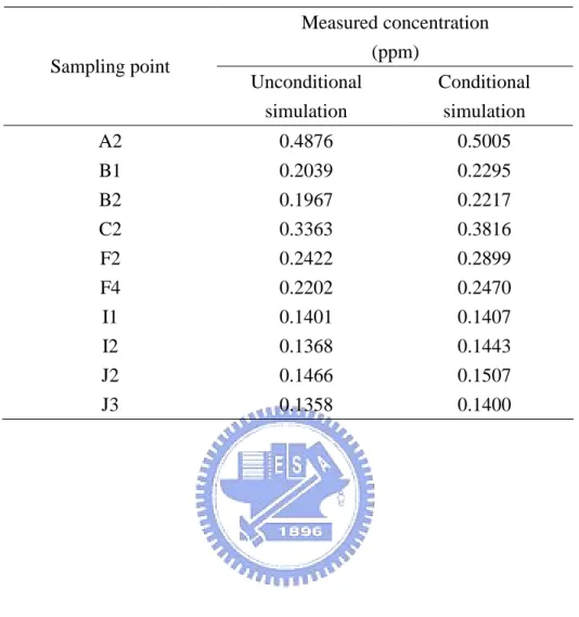
(32) CHAPTER 5 Examples and Results. 5.1 Numerical Examples An example is assumed for illustrating the source information estimation procedure. The example assumes that a point source S1 releases the contaminant in an unconfined aquifer.. The contaminant is assumed no decay and is not adsorbed on. the aquifer. The aquifer length and width are both 1000 m, and the aquifer thickness is 24 m.. The hydraulic conductivity, porosity, specific storage, and the hydraulic. gradient are, respectively, given as 15 m/day, 0.3, 10-4, and 0.005. Accordingly, the average groundwater flow velocity for a homogeneous aquifer under steady and uniform flow condition is 0.25 m/day and the dispersion coefficients in x-, y-, and zdirection are respectively given as 10 m2/day, 2.5 m2/day, and 0.25 m2/day.. The. finite difference grids are block-centered and the related boundary conditions for the flow field of the unconfined aquifer system are shown in Figure 4.. The grid width. and length are 40 m and the grid height is 6 m; thus, the number of finite difference mesh is 25 x 25 x 4.. The origin of the vertical coordinate is taken at the land surface. and S1 is located at (220 m, 540 m, -9 m). The S1, located at the depth of 9 m below the land surface, releases a constant concentration of 100 ppm over three-year with a release rate (W) of 1 m3/day.. The concentration, or called measured concentrations,. 21.

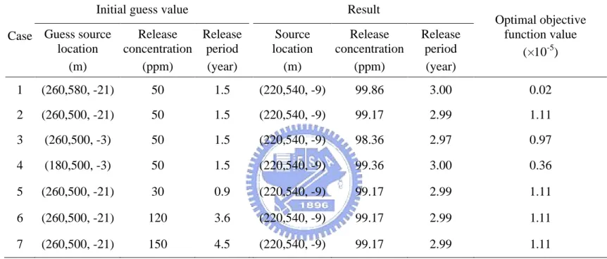
(33) at ten sampling points, i.e. wells A to J, shown in Figure 4 are simulated using MODFLOW-GWT.. Nineteen sampling points with various depths are considered. from these 10 sampling points. points are listed in Table 1.. The measured concentrations at these sampling. Note that the name of the sampling points given in. Table 1 consists of the well name and layer number.. For example, the sampling. point A2 represents the groundwater is sampled at the second layer of the monitoring well A. At the beginning of the source information estimation, totally 36 candidate sources, including the real source S1 and the suspicious source near S1 at different depths are considered.. The NS, NT, initial temperature and temperature reduction. factor are given as 20, 10, 5 and 0.8 respectively. The maximum numbers of location that tabu list memorized is three.. 5.2 Eight Scenarios and Results Eight scenarios are designed to test the applicability and validity of the proposed approach and the results are analyzed to extract a guideline for more effectively estimating the source information. The first scenario is to study the effect of using different initial guesses on the estimated results of the source location, release concentration, and release period. The second scenario is to explore the effect of the upper bound values of the release concentration and release period on the analyzed 22.

(34) results.. The third scenario is to examine the validity of the proposed approach when. the measured concentrations contain measurement errors with different measurement error level.. In the fourth scenario, three to seven sampling points are chosen to. investigate the required number of the sampling points.. The fifth scenario is. designed to extract a general guideline for allocating the sampling points in source information estimation.. Note that the depths of the source and measurement points. are assumed the same.. This implies that the depth of the source is known before. installing the sampling points and source information estimation in scenarios 1 - 5. Following scenarios are suitable for cases that the depth of the source location is not known. The sixth scenario uses 16 cases with different number and location of the sampling points to verify the guideline drawn from previous scenario.. In the seventh. scenario, four different depths of the source: 3m, 9m, 15m, and 21m below the land surface, are considered to explore the effect of the source depth on the allocation of the sampling points and the source information estimation.. The final scenario is to. study whether the guideline is also capable for the heterogeneous aquifer or not.. The. initial guess location for the source is (260 m, 500 m, -21m) and the initial guess value for the release concentration and release period are respectively 50 ppm and 1.5 years for scenarios 2 to 7.. Totally 4 different initial locations and 4 values of release. concentration and release period are chosen as the initial guess in the first scenario to. 23.

(35) test its effect on the source information estimation.. Excepted for the second scenario,. the upper bound values of release concentration and release period given in those scenarios are respectively 200 ppm and 6 years.. Three different upper bound values. for release concentration and release period are chosen in the second scenario to test their effect on the source information estimation.. 5.2.1 Scenario 1: Initial guesses for the source information One of the advantages of applying the global optimization approaches is that the initial guess values have little influence on the results of source information estimation.. This scenario contains seven cases to study the effect of using different. initial guesses on the estimated results of the source location, release concentration, and release period.. For cases 1 to 4, Table 2 shows the results when varying the. guess source location with initial guess values of 50 ppm and 1.5 years for the release concentration and release period, respectively.. The estimated source located at. (220m, 540m, -9m) is exact and the results of the release concentration and release period are slightly different from the real solution.. Case 4 give the worst results. which has 1.64% relative error in the estimated release concentration and 1% relative error in the estimated release period. For cases 5 to 7 the guess source is located at (260m, 500m, -21m), the guess values for the release concentration are given as: 30, 120, and 150 ppm, and the guess 24.

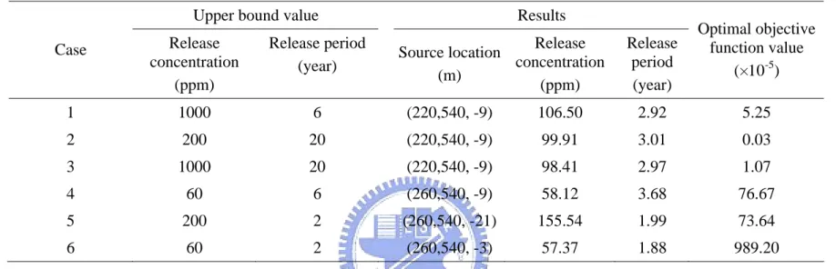
(36) values for the release period are given as 0.9, 3.6, and 4.5 years.. Table 2 also shows. the estimated results for the source location, release concentration, and release period are identical in these three cases.. The estimated source location is (220m, 540m,. -9m), the value of estimated release concentration is 99.17 ppm, and the estimated release period is 2.99 years, indicating that the estimated source location is correct and the results of the release concentration and release period just slightly differ from the real solution. In sum, those results indicate that the proposed approach is capable of estimating the source information regarding to the three-dimensional groundwater transport.. In. addition, these results also indicate that the proposed approach gives good estimate results while employing various guess values for the source location, release concentration, and release period.. 5.2.2 Scenario 2: Upper bound of the solution domain In our approach, the initial guesses and the upper and lower bounds must be given. If the upper bound values for the release concentration and release period are too low, the real solution may not fall within the upper and lower bounds.. In contrast, if the. upper bound values for the release concentration and release period are too high, the computing time to obtain the estimated results will be large. Six cases are designed for studying the effect of the upper bound values on the 25.

(37) analyzed results.. In cases 1 to 3, larger upper value such as 1000 ppm for release. concentrations and 10 year for release period are considered.. Table 3 shows the. estimated source location obtained in cases 1 to 3 are correct and the estimated release concentration and period are also in good accuracy.. Case 1 gives a slightly large. relative error among those three cases, i.e., 6.50% error in release concentration and 8.1% error in the release period. Therefore, we conclude that the effect of large upper bound values on the accuracy of source information estimation is insignificant. In cases 4 to 6, the upper bound values of the release concentration or/ and release period are smaller than the real ones to explore the effect of small upper bound values on the source information estimation. The upper bound values such as 60 ppm for release concentrations or/and 2 year for release period are considered in these three cases. Table 3 shows that the estimated source locations in these three cases are all incorrect and the values of release concentration or/and release period are close to the upper bound values.. For cases 4 and 6, the upper bound value of release. concentration is 60 ppm, and the estimate release concentrations obtained from these two cases are 58.12 ppm and 57.37 ppm, respectively.. For cases 5 and 6, the upper. bound value of release period is 2 year and the estimate release periods obtained from these two cases are 1.99 years and 1.88 years, respectively.. Besides, the optimal. objective function values obtained from the three cases are very high, i.e., larger than. 26.

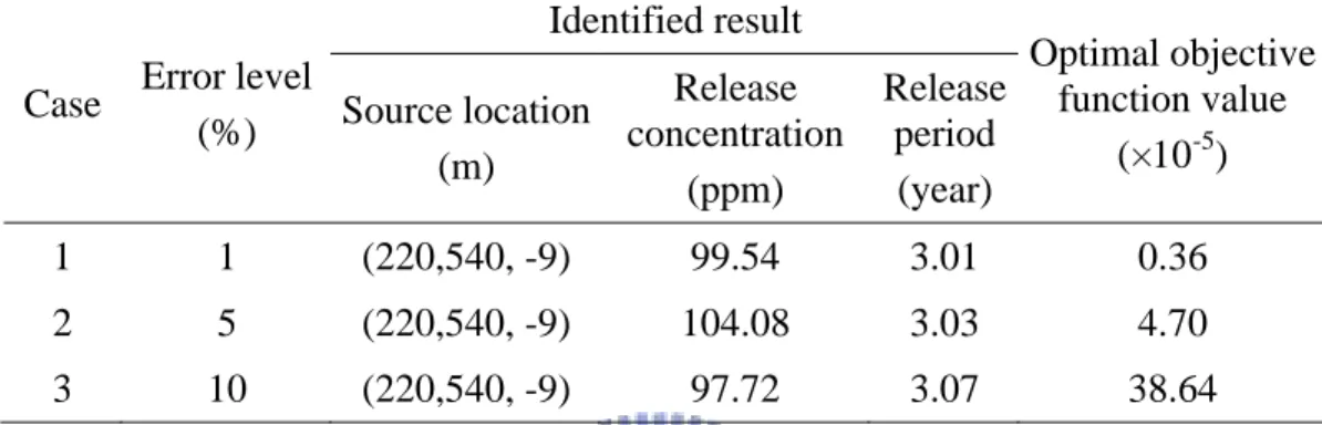
(38) 10-3.. Large objective function value reflects that the simulated concentrations are. significantly different from the measured concentrations.. Obviously, inappropriate. upper bound values made in the source information estimation give wrong results.. 5.2.3 Scenario 3: Measurement error In this scenario, random measurement errors are added into measured concentrations.. The disturbed measured concentrations are expressed as (Mahar and. Datta 2001):. Ci', obs = Ci , obs × (1 + E × RD4 ). (11). where C i',obs is the disturbed measured concentration, E is the level of measurement error, and RD4 is a random standard normal deviate generated by the routine RNNOF of IMSL (2003).. Three cases with the values of 1%, 5%, and 10% for E are. designed for this scenario. The estimated results shown in Table 4 indicate that the source locations are correct and the relative errors of the estimated release concentration and period between are small.. Even the measurement error level increases to 10%, the. estimated release concentration is 97.72 ppm, which only has a relative error of 2.28%. These results indicate that the proposed approach is applicable even the measured concentrations contain measurement error level up to 10%.. 27.

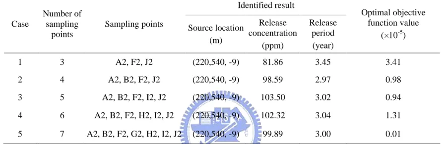
(39) 5.2.4 Scenario 4: Number of sampling points Five cases with sampling point numbers of 3 to 7 are considered in this scenario to explore the effect of the number of sampling points on the results of source information estimation.. Table 5 indicates that the estimated source location in these. 5 cases is correctly identified.. In addition, the obtained release concentration and. release period have very good accuracy, except in case one. The unknown variables involved in solving the problem of source information estimation include the source location, the released concentration, and release period. Mathematically, at least three sampling points are required to solve such a problem. However, the source location involves three dimensions, i.e., three coordinate values are needed to specify the source location.. Thus, five unknown variables are. involved in source information estimation.. This fact implies that 5 monitoring. points are sufficient to handle our source information problem with totally 5 unknowns. One might expect that adding more measured concentrations provide more information and may be helpful in estimating the source information. Table 5 shows that the differences of the results obtained from cases 3 to 5 are very small, indicating that the sixth and seventh sampling points employed in cases 4 and 5 provide very little improvement in the estimation results.. Notice also that in case 1. the number of the sampling points is three which is insufficient to determine the. 28.

(40) problem with 5 unknowns.. The relative error for the estimated release concentration. is 18.14% and for the estimated release period is 15% although the estimated source location is correct.. Accordingly, the number of sampling points for solving the. source information estimation problem in a homogeneous and isotropic site should be five at least.. 5.2.5 Scenario 5: A guideline for effectively estimating source information The purpose of this scenario is to draw a guideline to effectively estimate the source information.. Eleven cases are designed to explore the influence of the. magnitude of the measured concentrations on the estimated result.. In those cases,. five sampling points are chosen but the locations of the selected sampling points are varied.. Table 1 shows that the measured concentrations at the sampling points vary. from 0.0815 ppm to 0.4877 ppm.. Such a concentration distribution may be divided. into five different zones with a concentration difference of 0.1 ppm. Accordingly, the measured concentration ranging between 0 ppm and 0.1 ppm belongs to the first concentration zone and the measured concentration ranging between 0.4 ppm and 0.5 ppm belongs to the fifth concentration zone.. Table 6 lists the locations of the five. sampling points and the numbers of concentration zones, which are counted based on the measured concentrations at those five sampling points. Accordingly, case 1 has two zones, cases 2 – 6 have three zones, cases 7 – 10 have four zones, and case 11 has 29.

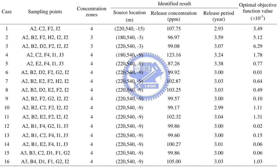
(41) five zones. Table 6 indicates that the estimate source location obtained from cases 1, 3, 5, and 6 are incorrect and those of cases 7 - 11 are correct, indicating that the values of measured concentration could influence the source information estimation.. As. indicated in the Table 6, one can observe that four out of six cases get wrong results when the number of measured concentration zones is equal to or less than three.. On. the other hand, the results obtained from those cases with four or more concentration zones are excellent. Four or more concentration zones may portray a better and clear feature for representing the spatial concentration distribution.. This result leads to. draw a guideline that when solving the source information estimation problem, at least five sampling points with four concentration zones are needed to ensure good source information estimation.. 5.2.6 Scenario 6: Guideline verification Sixteen cases are designed in this scenario to verify the guideline drawn from previous scenario.. The sampling points, the number of concentration zone, and the. identified results for these 16 cases are demonstrated in Table 7.. In case 1, four. sampling points are select and their related number of the concentration zones is four. In cases 2 and 3, the number of sampling points is six and the number of concentration zones is three. Table 7 indicates that the estimated source locations 30.

(42) for those three cases are incorrect. Notice that the number of sampling points in cases 2 and 3 is six which is more than the required sampling point number of five. These three cases demonstrate that the guideline of requiring at least five sampling points and four concentration zones is valid in source information estimation when the source and sampling points are located at the same depth. In cases 4 and 5, the number of sampling points is five and the number of concentration zones is five, but the depths of sampling points are varied.. Previous. studies focus on the problems that the source and sampling points are located at the same depth.. These two cases are to test the guideline when the sampling points are. not installed at the same depth.. As shown in Table 7, the estimated source locations. in these two cases are incorrect, indicating that the guideline fails as the sampling points are not installed at the same depth with the source location. In cases 6 to 11, the number of sampling points is increased to six and the number of concentration zones is still four. Note that those six sampling points are installed at different locations.. The purpose of these six cases is to verify the validity of the. guideline, when four concentration zones are chosen from different sets of sampling points.. Table 7 shows that the identified source locations are correct and the. estimated release concentration and release period are in good accuracy in those six cases.. It is important to point out that case 2 becomes case 9 and the number of. 31.

(43) concentration zone increases from three to four when the sampling point of H2 is replaced by G2.. Similarly, case 3 becomes case 8 and the number of concentration. zone increases from three to four when the sampling point of J2 is replaced by E2. The source information estimation fails in cases 2 and 3 but successes in cases 9 and 8. To ensure the applicability of the proposed approach, the requirement of six sampling points with four concentration zones are considered as the new guideline. For cases 12 to 16, case 12 has the same sampling location in x- and ycoordinates as the case 9 but differ in depth.. Similar arrangements are applied to. case 13 versus case 10 and case 14 versus case 11.. Note the sampling points. allocated at the first, third, and fourth layers have the same locations for cases 12 -14. Thus, the sampling points in cases 15 and 16 are installed at depths differing from those of cases 12 to 14. Table 7 shows that the sampling points in these five cases are distributed at four different depths of the aquifer and the identified source locations are correct and the estimated release concentration and release period have good accuracy. Notice that case 4 becomes case 13 and the number of concentration zone increases from three to four when the sampling point of B1 is added into case 4. Likewise, case 5 becomes case 14 and the number of concentration zone increases from three to four when the sampling point of B1 is added into case 5.. The source. information estimation fails in cases 4 and 5 but successes in cases 13 and 14.. 32.

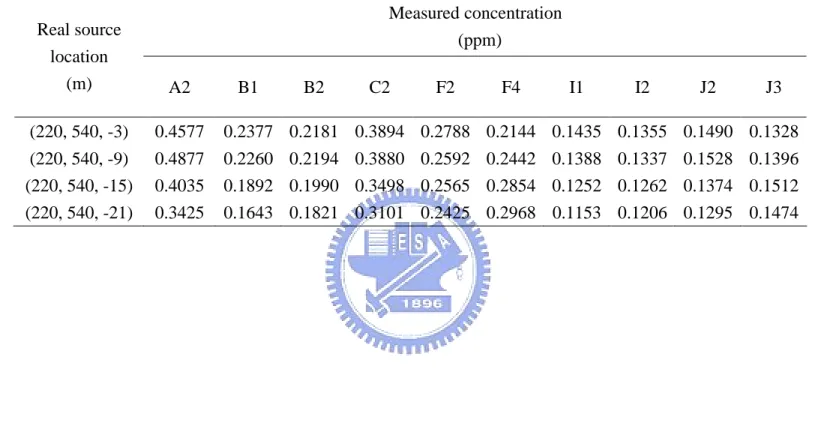
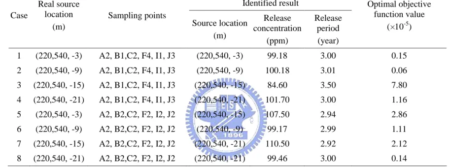
(44) Accordingly, it is to conclude that the new guideline of requiring six sampling points with four concentration zones is also valid even when the sampling points are installed at various depths.. 5.2.7 Scenario 7: Depth of source and well allocation Table 8 shows the measured concentrations obtained from ten sampling points while four real sources are located at different depth.. Eight cases including four real. sources located at different depths and two sets of monitoring well system are considered in this scenario, i.e., those four real sources are respectively located at -3m, -9m, -15m, or -21m, and the depth of the sampling points may be the same or different in the monitoring well system.. These eight cases are designed to explore. the effect of the source depths and well allocation on the results of source identification.. In the first four cases, the real sources, having four different depths,. are considered for source identification with the same five sampling points installed at various depths.. In the other four cases, four real sources located at different depths. are considered but the sampling points are installed at the same depths. The depths of real source and sampling points for each case and their analyzed results are listed in Table 9. Table 9 shows that the source locations obtained from cases 1 to 4 are correct and the release concentration and release period agree with the real solution. 33. This.

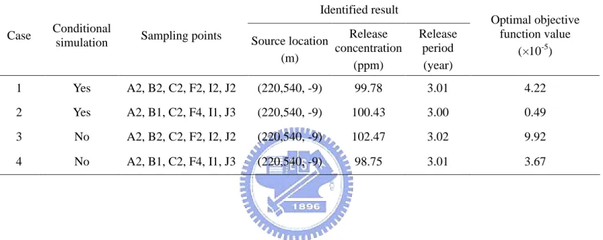
(45) indicates that the proposed approach works well when the sampling points are installed at different depths and the source location is not known. On the other hand, the results obtained from cases 5 to 8, while all the sampling points are installed at the same depth, indicate that cases 6 and 8 get good results and cases 5 and 7 obtain incorrect estimation for source location.. Therefore, we suggest that it had better to. install the sampling points at different depth to obtain the reliable identification results if the real source depth is unknown.. On the other hand, good results can be obtained. if one installs the sampling points at the same depth if the source depth is known in prior.. 5.2.8 Scenario 8: Heterogeneous aquifer In this scenario, the validity of the new guideline is verified when applying the proposed approach for the identification of contaminant source in a heterogeneous and isotropic aquifer.. A hypothetical heterogeneous aquifer is assumed and the. distribution of hydraulic conductivity of the heterogeneous aquifer is considered as a spatially-correlated and log-normally distributed random field.. The conductivity. field is generated by the program anneal of the geostatistical software, GSLIB (Deutsch and Journel, 1998). The correlation lengths in both x- and y- coordination are chosen as 200 m and the mean and standard deviation of the natural logarithm of hydraulic conductivity are 2.71, and 1.0 m/day, respectively. 34.

(46) Field aquifer tests such as slug test or pumping test are usually used to determine hydrogeologic parameters, i.e., hydraulic conductivity and storativity.. These aquifer. parameters obtained at specific locations can be used as conditional information. Assume that the hydraulic conductivities at wells A, B, C, F, I, and J obtained by aquifer tests are 17.481, 13.190, 13.167, 14.583, 15.888, and 17.171 m/day, respectively.. Four cases are designed in this scenario, spatially-correlated and. log-normal random conductivity fields are generated with known conductivity values mentioned above for cases 1 and 2 and without conditioning for cases 3 and 4.. All. sampling points are installed at the same depth in case 1 but at different depths in case 2.. The same example employed before except with a heterogeneous conductivity. field is considered herein to simulate the concentration distribution using MODFLOW-GWT.. The simulated results for the measured concentrations at the. sampling points are given in Table 10 for a conditional heterogeneous conductivity field.. Table 11 shows that the identified source locations are correct and the relative. errors of estimated release concentration and release period are less than 1% in both cases 1 and 2. The differences between the estimated release concentration and release period obtained in these two cases are also very small. For cases 3 and 4, the sampling points are installed at the same depth in case 3 but at different depths in case 4. The simulated results for the measured concentrations. 35.

(47) at the sampling points are also given in Table 10 for a heterogeneous conductivity field without conditioning. Table 11 indicates that the estimate source locations obtained from cases 3 and 4 are also correct and the estimated release concentration and release period are also in good accuracy.. The results obtained in this scenario. indicate that the new guideline is also capable for heterogeneous aquifers.. 36.

(48) Chapter 6 Conclusions. In this thesis, a new approach combines SA and TS to incorporate a three-dimensional groundwater flow and solute transport model, MODFLOW-GWT, for solving the source identification problem.. In the proposed approach, TS is. employed to generate the candidate source locations and SA is employed to generate the release concentration and release period at the candidate source location. MODFLOW-GWT. is. employed. to. simulate. the. three-dimensional. The plume. concentrations at the monitoring wells. The effects of the values of initial guess and measurement error on the results when employing the proposed approach to perform source information estimation are studied.. The proposed approach is also employed. to investigate the requirements for the optimal number of sampling points and the conditions for effectively estimating source information.. In addition, a guideline to. optimally allocate the sampling points in the estimation of source information for an aquifer with steady-state groundwater flow is suggested.. Six conclusions can be. drawn in this study. First, the approach we developed is capable for solving the three-dimensional groundwater source information estimation problem in both homogeneous and heterogeneous aquifer and the estimated results obtained from this study are similar. 37.

(49) and accurate.. Second, the identification results of the source location, release. concentration, and release period are independent on the initial guess, indicating that an inexperienced investigator could use this approach to estimate source information. Third, the effect of large upper bound values on the accuracy of source information estimation is insignificant.. In contrast, small upper bound value may give wrong. results if the real source is located outside the upper bound.. Fourth, the proposed. approach is applicable even the measured concentrations contain measurement error level up to 10%.. Fifth, it is found that at least five sampling points with four. concentration zones are needed to ensure good source information estimation if the both the source and sampling points are located at the same depths.. However, six. sampling points with four concentration zones is required when the sampling points are installed at various depths.. Finally, we suggest installing the sampling points at. different depth to obtain the reliable identification results if the real source depth is unknown.. 38.

(50) Reference. Altmann-Dieses, A. E., J. P. Schlo¨der, H. G. Bock, and O. Richter, (2002), Optimal experimental design for parameter estimation in column outflow experiments Water Resour. Res. 38(10), doi:10.1029/2001WR000358. Aral, M. M. and J. Guan, (1996), genetic algorithms in search of groundwater pollution sources. Advances in Groundwater Pollution Control and Remediation, 347-369. Aral, M. M., J. Guan, and M. L. Maslia ( 2001), Identification of Contaminant Source Location and Release History in Aquifers, Journal of Hydrologic Engineering, 6(3), 225-234. Atmadja J., A. C. Bagtzoglou, (2001), State of the art report on mathematical methods for groundwater pollution source identification. Environmental Forensics; 2: 205-214. Bagtzoglou, A. C., D. E. Kougherty, A. F. B. Tompson, (1992), Applications of particle methods to reliable identification of groundwater pollution sources. Water Resour. Mgmt. 6: 15-23. Cleveland, T.G., W. W-G. Yeh, (1991), Sampling network design for transport parameter identification, J. Water Resour. Plng. And Mgmt., ASCE 116(6): 764-783. Cunha, M.D.C., J. Sousa (1999), Water distribution network design optimization: simulated annealing approach, J. Water Resour Plng and Mgmt, ASCE 1999; 125(4): 215-221. Glover, F., (1986), Future path for integer programming and links to artificial intelligence, Computers and Operation Research, 13: 533-549.. 39.

(51) Gorelick, S. M., B. Evans, and I. Remson (1983), “Identifying sources of groundwater pollution: An optimization approach.” Water Resour. Res., 19(3) 779-790. Harbaugh, A.W., E.R. Banta, M.C. Hill, and M.G. McDonald, (2000), MODFLOW-2000, the U.S. Geological Survey modular ground-water model User guide to modularization concepts and the Ground-Water Flow Process, U.S. Geological Survey Open-File Report 00-92. Hsu, N-S, W. W-G Yeh, (1989), Optimum experimental design for parameter identification in groundwater hydrology Water Resour. Res. 25(5): 1025-1040. Hwang, J. C. and R. M. Koerner (1983), “Groundwater pollution source identification from limited monitoring well data: part I – theory and feasibility”, Journal of Hazardous Materials, 8, 105-119. IMSL (2003), Fortran Library User’s Guide Stat/Library, Volume 2 of 2, Visual Numerics, Inc., Houston, TX. Jeong, I.K., J.J. Lee, (1996) Adaptive simulated annealing genetic algorithm for system identification, Engng Applic. Artif. Intell. 9(5): 523-532 Knopman, D.S., C.I. Voss, (1989), Multiobjective sampling design for parameter estimation and model discrimination in groundwater solute transport Water Resour. Res. 25(10): 2245-2258. Knopman, D.S., C.I. Voss, S. Garabedian, (1991) Sampling design for groundwater solute transport: test of methods and analysis of Cape Cod trace test data Water Resour. Res. 27(5): 925-949. Konikow, L.F., D.J. Goode, and G.Z. Hornberger, (1996), A three-dimensional method of characteristics solute-transport model (MOC3D), U.S. Geological Survey Water-Resources Investigations Report 96-4267. Liu C., W.P. Ball, (1999), Application of inverse methods to contaminant source identification from aquitard diffusion profiles at Dover AFB, Delaware. Water 40.

(52) Resour. Res. 35(7): 1975-1985. Loaiciga H.A., R.J. Charbeneau, L.T. Everett, G.E. Fogg, B.F. Hobbs, S. Rouhani, (1992) review of ground-water quality monitoring network design Journal of hydraulic engineering 18(1): 11-37. Mahar, P. S., and B. Datta (1997), Optimal monitoring network and ground-water-pollution source identification J. Water Resour. Plng. And Mgmt. ASCE, 123(4), 199-207. Mahar, P. S. and B. Datta (2000), Identification of pollution sources in transient groundwater systems Water Res. Man. 14(3), 209-227. Mahar, P. S. and B. Datta (2001), Optimal identification of groundwater pollution sources and parameter estimation J. Water Res. Pl., 127, 20-29. Metropolis, N., A.W. Rosenbluth, M.N. Rosenbluth, A.H. Teller, and E. Teller (1953), Equation of state calculations by fast computing machines J. of Chem. Phys. 21(6),1087-1092. National Research Council, (1990), Groundwater models – Scientific and Regulatory Applications, National Academy Press, Washington D. C. Neupauer R. M., B. Borchers, J. L. Wilson, (2000), Comparison of inverse methods for reconstructing the release history of a groundwater contamination source. Water Resour. Res. 36(9): 2469-2475. Neupauer R. M., J. L. Wilson, (1999) Adjoint method for obtaining backward-in-time location and travel time probabilities of a conservative groundwater contaminant. Water Resour. Res. 35(11): 3389-3398. Neupauer R. M., J. L. Wilson, (2001), Adjoint-derived location and travel time probabilities for a multi-dimensional groundwater system. Water Resour. Res. 37(6): 1657-1668. Nishikawa T., W. W-G Yeh, (1989), Optimal pumping test design for the parameter 41.

(53) identification of groundwater systems Water Resour. Res. 25(7): 1737-1747. Pham, D.T. and D. Karaboga (2000), “Intelligent Optimisation Techniques”, Springer, Great Britain. Samarskaia, E., (1995), Groundwater contamination modeling and inverse problems of source reconstruction. Systems Analysis Modelling Simulation, 18-19: 143-147. Sciortino A., T-C. Harmon, W. W-G. Yeh, (2000), Inverse modeling for location dense nonaqueous pools in groundwater under steady flow conditions Water Resour. Res. 36(7): 1723-1735. Sciortino A., T-C. Harmon, W. W-G. Yeh, (2002) Experimental design and model parameter estimation for location a dissolving dense nonaqueous phase liquid pool in groundwater Water Resour. Res. 38(5): 15-1-10. Skaggs T. H., Z. J. Kabala, (1994) Recovering the release history of a groundwater contaminant. Water Resour. Res. 30(1): 71-79. Skaggs T. H., Z. J. Kabala, (1995) Recovering the history of a groundwater contaminant plume: Method of quasi-reversibility. Water Resour. Res. 31(11): 2669-2673. Skaggs T. H., Z. J. Kabala, (1998) Limitations in recovering the history of a groundwater contaminant plume. J. Contam. Hydrol. 33: 347-359. Snodgrass M. F., P. K. Kitanidis, (1997) A geostatistical approach to contaminant source identification. Water Resour. Res. 33(4): 537-546. Sun N-Z, W. W-G Yeh, (1985), Identification of parameter structure in groundwater inverse problem Water Resour. Res. 21(6): 869-883. Tung C. P., C. A. Chou., (2004), Pattern Classification with Tabu Search to Identify Spatial Distribution of Groundwater Pumping Hydrogeology Journal 12(5): 488-496 42.

(54) Tung C. P., C. C. Tang, Y. P. Lin., (2003), Improving groundwater flow modeling using optimal zoning methods Environmental Geology 44: 627~638. Wagner, B.J., (1992) Simultaneous parameter estimation and contaminant source characterization for coupled groundwater flow and contaminant transport modelling. J. Hydrol. 135: 275-303. Woodbury A., E. Sudicky, T.J. Ulrych, R. Ludwig, (1998) Three-dimensional plume source reconstruction using minimum relative entropy inversion. J. Contam. Hydrol. 32:131-158. Woodbury A. D., T. J. Ulrych, (1996) Minimum relative entropy inversion: theory and application to recovering the release history of a groundwater contaminant. Water Resour. Res. 32(9): 2671-2681. Zheng C., P. Wang, (1996) Parameter structure identification using tabu search and simulated annealing, Adv. Water Res. 19(4): 215-224. 43.

(55) Table. 1 The sampling points and the measured concentrations for the homogeneous aquifer when the real source is located at the depth of -9 m.. Sampling point. Measured concentration (ppm). A2 A3 B1 B2 B3 B4 C2 D1 D2 E2 F1 F2 F4 G2 H2 I1 I2 J2 J3. 0.4877 0.4029 0.2260 0.2194 0.1993 0.1828 0.3880 0.2279 0.2206 0.0815 0.2903 0.2592 0.2442 0.0564 0.1342 0.1388 0.1337 0.1528 0.1396. 44.

(56) Table 2 The results of 7 cases designed in the first scenario for studying the effect of initial guesses on source information estimation Result. Initial guess value Release Release Case Guess source concentration period location (year) (m) (ppm). Source location (m). Release concentration (ppm). Release period (year). Optimal objective function value (×10-5). 1. (260,580, -21). 50. 1.5. (220,540, -9). 99.86. 3.00. 0.02. 2. (260,500, -21). 50. 1.5. (220,540, -9). 99.17. 2.99. 1.11. 3. (260,500, -3). 50. 1.5. (220,540, -9). 98.36. 2.97. 0.97. 4. (180,500, -3). 50. 1.5. (220,540, -9). 99.36. 3.00. 0.36. 5. (260,500, -21). 30. 0.9. (220,540, -9). 99.17. 2.99. 1.11. 6. (260,500, -21). 120. 3.6. (220,540, -9). 99.17. 2.99. 1.11. 7. (260,500, -21). 150. 4.5. (220,540, -9). 99.17. 2.99. 1.11. Note that the real source is located at (220m, 540m, -9m), real release concentration is 100 ppm, real release period is 3 years, and the sampling points contain A2, B2, C2, F2, I2, J2.. 45.

(57) Table 3 The results of 6 cases designed in the second scenario for the examination of the solution domain Upper bound value. Results. Case. Release period (year). 1. 1000. 6. (220,540, -9). 106.50. 2.92. 5.25. 2. 200. 20. (220,540, -9). 99.91. 3.01. 0.03. 3. 1000. 20. (220,540, -9). 98.41. 2.97. 1.07. 4. 60. 6. (260,540, -9). 58.12. 3.68. 76.67. 5. 200. 2. (260,540, -21). 155.54. 1.99. 73.64. 6. 60. 2. (260,540, -3). 57.37. 1.88. 989.20. Release Source location concentration (m) (ppm). Release period (year). Optimal objective function value (×10-5). Release concentration (ppm). Note that the real source is located at (220m, 540m, -9m), real release concentration is 100 ppm, real release period is 3 years, and the sampling points contain A2, B2, C2, F2, I2, J2.. 46.

(58) Table 4 The results of 3 cases designed in the third scenario for the effect of measurement error on source information estimation Identified result Case. Error level Release Release Source location (%) concentration period (m) (ppm) (year). Optimal objective function value (×10-5). 1. 1. (220,540, -9). 99.54. 3.01. 0.36. 2. 5. (220,540, -9). 104.08. 3.03. 4.70. 3. 10. (220,540, -9). 97.72. 3.07. 38.64. Note that the real source is located at (220m, 540m, -9m), real release concentration is 100 ppm, real release period is 3 years, and the sampling points contain A2, B2, C2, F2, I2, J2.. 47.

(59) Table 5 The results for 5 cases designed in the fourth scenario for the examination of the number of sampling points Identified result. Optimal objective function value (×10-5). Case. Number of sampling points. Sampling points. 1. 3. A2, F2, J2. (220,540, -9). 81.86. 3.45. 3.41. 2. 4. A2, B2, F2, J2. (220,540, -9). 98.59. 2.97. 0.98. 3. 5. A2, B2, F2, I2, J2. (220,540, -9). 103.50. 3.02. 0.94. 4. 6. A2, B2, F2, H2, I2, J2. (220,540, -9). 102.32. 3.04. 1.31. 5. 7. A2, B2, F2, G2, H2, I2, J2. (220,540, -9). 99.89. 3.00. 0.01. Release Source location concentration (m) (ppm). Release period (year). Note that the real source is located at (220m, 540m, -9m), real release concentration is 100 ppm, and real release period is 3 years.. 48.

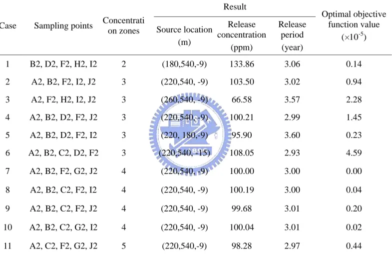
(60) Table 6 The results of 11 cases designed in the fifth scenario to find the guideline for effectively source information estimation Result. Optimal objective function value (×10-5). Case. Sampling points. Concentrati on zones. 1. B2, D2, F2, H2, I2. 2. (180,540,-9). 133.86. 3.06. 0.14. 2. A2, B2, F2, I2, J2. 3. (220,540, -9). 103.50. 3.02. 0.94. 3. A2, F2, H2, I2, J2. 3. (260,540, -9). 66.58. 3.57. 2.28. 4. A2, B2, D2, F2, J2. 3. (220,540, -9). 100.21. 2.99. 1.45. 5. A2, B2, D2, F2, I2. 3. (220, 180,-9). 95.90. 3.60. 0.23. 6. A2, B2, C2, D2, F2. 3. (220,540, -15). 108.05. 2.93. 4.59. 7. A2, B2, F2, G2, J2. 4. (220,540, -9). 100.00. 3.00. 0.00. 8. A2, B2, C2, F2, I2. 4. (220,540, -9). 100.19. 3.00. 0.04. 9. A2, B2, C2, F2, J2. 4. (220,540, -9). 99.68. 3.01. 0.20. 10. A2, B2, C2, G2, I2. 4. (220,540, -9). 100.04. 3.01. 0.02. 11. A2, C2, F2, G2, J2. 5. (220,540,-9). 98.28. 2.97. 0.44. Release Source location concentration (m) (ppm). Release period (year). Note that the real source is located at (220m, 540m, -9m), real release concentration is 100 ppm, and real release period is 3 years.. 49.