Image Interpolation Using Spatial And Spectral Correlations

全文

(1)IMAGE INTERPOLATION USING SPATIAL AND SPECTRAL CORRELATIONS Wenmiao Lu and Yap-Peng Tan Division of Information Engineering School of Electrical and Electronic Engineering Nanyang Technological University Email: {ewmlu, eyptan}@ntu.edu.sg. ABSTRACT This paper presents a new method to interpolate digital color images by exploiting the spatial and spectral correlations inherent in the images. The proposed method involves two main steps: interpolating green image plane solely based on the local spatial correlation within the color plane, and interpolating red and blue image planes based on the spectral correlation between different color image planes. The performance of the proposed algorithm is evaluated by interpolating down-sampled color images back to their original image sizes and comparing the results with the original images as well as those generated by other existing image interpolation schemes. Experimental results show that the proposed method can better preserve valuable image attributes: edge sharpness and color consistency, which have great influence on the perceived visual quality of the interpolated images.. 1. INTRODUCTION Image interpolation is often required in many imaging applications for enlarging images or restoring lowresolution images to their original sizes. These include image zooming in digital imaging devices (such as digital camera, printer and scanner) and image sharing across heterogeneous, distributed multimedia systems [1]. As the reverse process of image down-sampling, a common means to reduce the spatial resolution of images for display, storage and transmission purposes, image interpolation aims to produce high-resolution images from their down-sampled versions. We present in this paper a new and improved method for interpolating color images to higher spatial resolution. The proposed method manages to generate interpolated images that can better preserve the sharpness of image edges and contain less interpolation artifacts, such as color bleeding. The method involves two main steps: interpolating the green image plane solely based on the local spatial correlation and interpolating the red and blue color planes based on the spectral (inter-color plane) correlation. Although we present our method in this paper using RGB (red-green-blue) color images, each of which consists of red, blue, and green image planes, it can be readily applied to color images recorded in different color. spaces or color components, such as YCbCr color space or Yellow-Cyan-Magenta color components. The rest of the paper is organized as follows. Section 2 provides a review of background theories and prior work on image interpolation. The overview of the proposed image interpolation algorithm is presented in Section 3. Section 4 describes the local spatial correlation based method for interpolating green image plane. Section 5 addresses the inter-color plane correlation-based method for interpolating red and blue image planes. The experimental results and their comparison with images produced by other interpolation methods are reported in Section 6. In Section 7, we conclude the paper.. 2. REVIEW OF BACKGROUND THEORIES AND PREVIOUS WORK Image interpolation, also known as image enlargement or image magnification, is normally used to increase the size or spatial resolution of images. Owing to its wide uses in many imaging applications, many linear and nonlinear image interpolation techniques have been proposed in the literature. Roughly, these techniques can be grouped into the following five main categories: 1. Single kernel based techniques that involve a convolution between low-resolution images and a 2D interpolation kernel, for example [1]. 2. Multiple kernel based techniques that work with a set of pre-defined interpolation kernels, for example [2]. 3. Transform based techniques that interpolate images in a transform domain using transform such as discrete cosine transform (DCT) or wavelet transform, for example [3]. 4. Optimization based techniques that formulate image interpolation as a constrained optimization problem minimizing a specific cost function, for example [4]. 5. Edge adaptive techniques that examine local image edge content and interpolate images in low frequency direction (along the edge), rather than in high frequency direction (across the edge), for example [5][6]. Brief summaries of these five categories of image interpolation techniques are provided in the following to serve as the literature review of our work..

(2) 2.1 Single kernel based image interpolation This type of interpolation involves a convolution between the observed image samples and a 2D kernel. The three most commonly used convolution kernels for image interpolation care the zero-order-hold, bilinear and bicubic kernels respectively. Zero-order-hold kernel is the simplest. Interpolation with this kernel is commonly referred to as nearest neighbor interpolation or pixel replication. Using this kernel, each unknown pixel is filled with the existing image pixel closest to its location. Due to this pixel replication, the zero-order-hold kernel usually produces images with a very ‘blocky’ image appearance. However, it is computationally simple and easy to be implemented. Bilinear interpolation kernel is composed of two 1D linear interpolation kernels. The kernel involves the four image pixels nearest to the pixel to be interpolated. It gives smoother image appearance compared to that of zero-order interpolation and demands moderate computational cost. Bicubic interpolation kernel locally fits a separable thirddegree polynomial through sixteen adjacent image pixels. The fitting constraints tend to limit the amount of oscillation across an image edge. It gives smooth image appearance and maintains some sharp details. However, it is the most computational expensive among these three common kernels. 2.2 Multiple kernels based image interpolation Multiple kernels based schemes examine local image structures in order to select an appropriate interpolation kernel for the pixel to be interpolated [2]. One set of kernels is usually pre-defined for the image interpolation, and the intensity structure of a local image neighborhood around the unknown pixel under consideration is analyzed to determine the most suitable interpolation kernel to be used. 2.3 Orthogonal transform based image interpolation Orthogonal transforms, such as discrete cosine transform (DCT) and wavelet transform, have often been used for image interpolation. Image interpolation using wavelet transform exploits the fact that the signal evolution across different resolution scales can be used to predict the image detail at finer scales. For DCT based interpolation, previous work has implemented digital filters to perform the required spatial domain filtering in the DCT domain. For example, Hong [3] uses the local DCT coefficients to identify five different types of image edges. Once the edge type is determined, a single linear kernel corresponding to the detected edge type is used to interpolate the image.. Low-resolution Image. Red plane. Green plane. Blue plane. Step 1: Local Covariance-based Green Plane Interpolation. Local Gradients Analysis on Interpolated Green Plane and Selection of Smooth Regions for Next Interpolation Step. Step 2: Inter-channel Correlation based Red, Blue plane interpolation. High-resolution Image. Figure 1: Overview of the proposed interpolation scheme. 2.4 Optimization based image interpolation Optimization techniques formulate image interpolation as a constrained optimization problem minimizing a specific cost function. The choice of the cost function to be minimized is based on a combination of the restrictions imposed by certain considerations corresponding to the physical problem. One representative work done by Ruderman and Bialek [4] shows that if the statistical property of a signal is known a priori, the observed signal samples can be used to estimate information beyond the Nyquist limit. They consider the interpolation a process of finding the “best” estimate of the original signal given the original signal statistics and the observed signal samples. They show that the optimal interpolation procedure for a Gaussian signal results in a convolution of the signal samples with an.

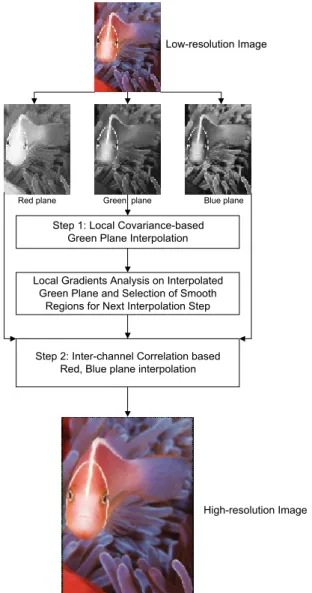
(3) interpolation kernel that is a function of the noise variance, the power spectrum, and the sampling rate of the original signal. 2.5 Edge adaptive image interpolation Edge adaptive interpolation techniques recognize the fact that it is desirable to interpolate image along the edge instead of across it. Jensen and Anastassiou [5] propose a method that detects the presence of high contrast edges and then interpolate the image along the edges. Bayrakeri and Mersereau propose a weighted directional interpolation scheme [6], where the values interpolated along various directions are combined with appropriate weightings based on the variations in different directions. 2.6 Remarks Due to their computational simplicity, image interpolation techniques with the use of a single linear interpolation kernel have been widely engaged in many imaging applications. However, natural images consist of multifold objects. The intensity of an image often changes abruptly across objects’ boundaries. Thus, applying convolution with a linear interpolation kernel indiscriminately throughout an image irrevocably blurs the image edges and introduces artifacts around them. To resolve this problem, many nonlinear interpolation techniques that perform interpolation adapted to local image structures have been proposed. Although some of them are well established for grayscale images, a direct extension of these techniques to color images may lead to undesirable interpolation artifacts, such as color bleeding. Besides, this also incurs unnecessary high computational cost, as the inherent correlation between different color image planes is not exploited [7]. With these considerations in mind, we have developed a new method for color image interpolation.. 4. GREEN IMAGE PLANE INTERPOLATION USING SPATIAL CORRELATION The first step of the proposed algorithm is to fully interpolate a high-resolution green plane. As the green plane of a RGB image contains most of the spatial details of the captured scene, it should be interpolated with closer attention in order to reconstruct as many image details as possible. This step is an extension of Li’s method [8], which is able to produce interpolated images with attractive perceptual quality. The step is based on the classical Wiener filtering that is well known to be capable of obtaining the optimal estimate of unknown data from a Gaussian random process [9]. Although it is computationally easier to assume that image intensities of a local spatial neighborhood tend to be stationary and can be well modeled with Gaussian distribution, this is often not the case for natural images. Natural images are usually populated with edges that can be better characterized by abrupt changes of local statistics. In other words, the classical Wiener filtering may not be able to produce optimal results around or across image edges. To cope with this problem, the proposed algorithm interpolates the high-resolution pixel from a group of pre-selected neighboring pixels, which and the pixel to be interpolated (also referred to as the unknown pixel) can be well modeled with a stationary Gaussian process. By performing edge detection within a local neighborhood, only the pixels residing at the same side of the edge as the pixel to be interpolated are engaged in the interpolation process. This is the main difference from Li’s method, which directly applies a covariance-based interpolator using all the available pixels around the pixels to be interpolated. Let us illustrate the idea with an example. In Figure 2, the low-resolution green image plane Gi, j and the. 3. ALGORITHM OVERVIEW. interpolated green image plane G~i , j of the image under. Figure 1 shows the overview of the proposed algorithm for interpolating low-resolution color images. It consists of two steps. First, the green image plane of a lowresolution color image is interpolated to the desired spatial resolution by exploiting the local spatial correlation within the green image plane. The fully interpolated green image plane is subject to gradient analysis in order to identify local image regions that are suitable for interpolating the red and blue pixel values. Second, within the selected image regions, the unknown red and blue values are interpolated based on the spectral correlation between different color image planes. The details of the proposed algorithm are presented in the following two sections.. consideration are living on an H × W lattice and an mH × nW lattice respectively, where m and n are the upscaling factors in the vertical and the horizontal image dimensions, respectively. Although our algorithm can be used to up-sample images by arbitrary integer factors, we shall describe the algorithm using the case of m = n = 2 ~ and G2i,2 j = Gi , j . The low-resolution green pixels, denoted by filled circles, are separated by an edge as illustrated in Figure 2. By examining the locations of the unknown pixel and the neighboring low-resolution pixels around the image edge detected, our proposed algorithm determines the side of the edge at which the unknown pixel lies. (Note that the diameters of the filled circles are altered to represent the values of the green pixels.).

(4) The unknown green pixel value at G~2i +1,2 j +1 is linearly estimated from its four nearest neighboring pixels (Figure 3: case 1) with equation ~ G 2i +1, 2 j +1 =. 1. 1. ∑∑ α. 2 k + l G 2 ( i + k ), 2 ( j + l ). Detected Edge. α1. (1). α2. k =0 l =0. v. where α = [α 1 , α 2 , α 3 , α 4 ]T are proper weightings for the neighboring pixels. By using Wiener filter, the weightings v α can be optimally estimated, in the sense of minimum mean-square error. It is equivalent to solving the following over-constrained linear equations: v v g = CT × α. (2). v v α = R −1 × r. (3). where R = CC T is the local covariance matrix and rv = Cgv is the covariance vector for the low-resolution pixels selected. The vector gv = [...g k ...]T contains the green values of the low-resolution pixels, which locate at the same side of the edge as the high-resolution pixel ~ G2i +1,2 j +1 to be interpolated. From this, the matrix C. whose kth column consists of the green values of four nearest low-resolution interpolating neighbors of g k can hence be constructed. To obtain the complete high-resolution green plane, we ~ apply the same algorithm to construct pixel G2 i +1, 2 j of the partially filled lattice. The only difference is that a diamond-shaped local window, as shown in Figure 3: case 2, is used to estimate the unknown pixel value. When no edge is found within a local image neighborhood, we revert to bilinear interpolation for the sake of simplicity. In comparison to Li’s method, the proposed technique can better preserve the fine details of image, such as short edges and isolated dots. Li applied a template of fixed size throughout the whole image and used all the lowresolution pixels inside the local windows to reconstruct the high-resolution images. It works fine for the long curved edges by smoothing along them. However, Li’s method will over-smooth the fine image details. Inside the local windows around these fine image details, most of the neighboring pixels, which dominate the interpolation process, possess the statistical properties different from that of the pixel to be interpolated. As a result, those fine image details are lost in the reconstructed images. On the contrary, our proposed method avoids this problem by pre-selecting similar neighboring pixels. Not only is the smoothness of the long curved edges ensured, but also the sharpness of the short edges is preserved. This can be clearly seen from Figure 4, where interpolation result generated by Li’s. α1. α4. α2. α3. α4 α3. g k : One of the pre-selected pixel. g k and its four interpolating neighbors. ~ G 2i +1,2 j +1 and its four interpolating neighbors. ~. : Low-resolution pixel G2 i , 2 j = Gi , j. ~ : Interpolated pixel G 2i +1, 2 j +1. : Pre-selected region which contains the v low-resolution pixels used to estimate optimal weightings α = [α 1 , α 2 , α 3 , α 4 ]T. ~. : Interpolated pixel G2 i +1, 2 j. Figure 2: Lattices for image interpolation. α1. α4. α4. α3. α1 α2. α3. ~. : Interpolated pixel G2 i 1, 2 j 1 + + Interpolation Case 1. α2. ~. : Interpolated pixel G2 i +1, 2 j. Interpolation Case 2. Figure 3: Pixel to be interpolated and its four nearest neighboring pixels.. (a) Result produced by the proposed method. (b) Result produced by Li's method. Figure 4: The images interpolated by (a) the proposed method and (b) Li’s method. method (posted on the web site of signal processing laboratory at Cornell University [11]) and the result generated by our proposed method are presented for visual comparison. Although the adaptive selection of neighboring pixels and linear estimation based on Wiener filtering incur relatively expensive computational cost, the interpolation results give superior edge preservation, which is critical to the following interpolation of red and blue image planes..

(5) 5. RED AND BLUE IMAGE PLANE INTERPOLATION USING SPECTRAL CORRELATION The red and blue image planes are interpolated by analyzing the fully interpolated green image plane. If the spatial correlation-based interpolator for the green plane is applied to up-sample the red and blue planes separately, very expensive computational cost will be incurred. Inspired by Chang’s color interpolation scheme for the Bayer’s CFA (Color Filter Array) pattern [10], we contrive an interpolator that exploits the spectral correlation between different color planes to construct the high-resolution red and blue image planes with less computation requirement and better color consistency. There are two underlying assumptions. First, the interpolated green plane contains sufficient gradient information for the complete color image. Second, within a given local image region, the differences between the red and green values of the neighboring image pixels are highly similar; this is also the case for the differences between the blue and green pixel values. The first assumption holds for most natural images, since the green image plane normally records the scene’s spectral energy in a way similar to the response of the human visual system. The second assumption is decent for most image regions and only fails with sharp image edges. To handle the exception due to sharp edges, only pixels in smooth image regions should be engaged in estimating the unknown red and blue pixel values. Specifically, the smooth image regions refer to those regions whose pixels have color values similar to the unknown pixel. These regions can be reasonably identified by using the local gradient information obtained from the interpolated green plane. Low gradient values indicate that the pixels have the similar color values, whereas high gradient values suggest that the pixels are from image regions with many details or sharp edges. The computation of local image gradients is performed within a 5-by-5 local window of the interpolated green image plane, as shown in Figure 4. The window is divided into eight regions corresponding to the eight directions (N, E, S, W, NE, SE, SW, NW).. G1. G6. G2, R2, B2. G7. G3. G8. G4, R4, B4. G9. G5. G10. G11 G12, R12, B12 G13, R13? B13? G14, R14, B14 G15. G16. G21. G17. G22, R22, B22. G18. G23. G19. G24, R24, B24. G20. G25. (1) Type A Location G1. G6. G11. G16. G21. G2. G7, R7, B7. G12. G17, R17, B17. G22. G3. G8. G13, R13? B13?. G18. G23. G4. G9, R9, B9. G14. G19, R19, B19. G24. G5. G10. G15. G20. G25. (2) Type B Location G1. G 6, R6, B6. G11. G16, R16, B16. G21. G2. G7. G12. G17. G22. G3. G 8, R8, B8. G13, R13? B13?. G18, R18, B18. G23. G4. G9. G14. G19. G24. G5. G10, G20, G15 R10, B10 R20, B20 (3) Type C Location. G25. Figure 5: Three types of locations where the pixel to be interpolated can reside. The local image gradient in each direction is computed by equations: Gradient_ N = G13 − G11 + G14 − G12 + G8 − G6 / 2 + G18 − G16 / 2;. G1. G6. G11. G16. G21. Gradient_ E = G13 − G23 + G8 − G18 + G12 − G22 / 2 + G14 − G24 / 2;. G2. G7. G12. G17. G22. Gradient_ S = G13 − G15 + G12 − G14 + G18 − G20 / 2 + G8 − G10 / 2;. G3. G8. G13. G18. G23. G4. G9. G14. G19. G24. G5. G10. G15. G20. G25. Figure 4: A 5-by-5 local window around pixel G13 of the interpolated green image plane.. Gradient_ W = G13 − G3 + G18 − G8 + G14 − G4 / 2 + G12 − G2 / 2; Gradient_ NE = G13 − G21 + G9 − G17 + G8 − G16 / 2 + G14 − G22 / 2; Gradient_ NW = G13 − G1 + G19 − G7 + G18 − G6 / 2 + G14 − G2 / 2; Gradient_ SE = G13 − G25 + G7 − G19 + G8 − G20 / 2 + G12 − G24 / 2; Gradient_ SW = G13 − G5 + G17 − G9 + G12 − G4 / 2 + G18 − G10 / 2; Local _ gradients= {Gradient_ N , Gradient_ E, Gradient_ S , Gradient_ W , Gradient_ NE, Gradient_ NW , Gradient_ SE, Gradient_ SW}. (4).

(6) where the image gradient in each region is computed by accumulating the absolute differences of green pixel values in the respective region. Instead of using two adjacent pixels, the difference between two alternate neighboring green pixels is computed to better capture the scene variation. The absolute differences are also properly weighted with weighting 1 or 0.5 according to their distances from the pixel under consideration. Once we have obtained the local image gradient in each direction, we identify the smooth image regions by comparing each gradient magnitude to a threshold defined as T = median{local_gradients} , where local _ gradients is the set of gradient magnitudes in the eight directions. Those regions with gradient magnitudes below this threshold are considered smooth. The pixels inside these smooth regions, which have complete RGB color values, are used to estimate the differences between the green pixel value and the unknown red/blue pixel value. Since the red and blue image planes are to be interpolated by a factor of two in each image dimension, there are three different cases, which depend on the location of the pixel to be interpolated, for estimating the differences between color values. The three types of locations are shown in Figure 5, where the red and blue color values of G13 are to estimated. Let us use an example to illustrate how to compute the unknown color values R13 and B13 . For instance, if the image local gradients computed from regions {S, W, SE, SW} are less than the threshold T = median{local _ gradients} , the pixels which have complete RGB color values and locate inside the regions {S, W, SE, SW} will be used to estimate R13 and B13 . For Type A location shown in Figure 5, the following table indicates the pixels used for estimating R13 and B13 . Red. Green. Blue. SE. R14 (R2+ R4+ R12+ R14)/4 (R14+ R24)/2. G14 (G2+ G4+ G12+ G14)/4 (G14+ G24)/2. B14 (B2+ B4+ B12+ B14)/4 (B14+ B24)/2. SW. (R4+ R14)/2. (G4+ G14)/2. (B4+ B14)/2. S W. The average color values for pixels in these four regions are computed as follows: Rave = [R14 + (R2 + R4 + R12 + R14 )/ 4 + (R14 + R24 )/ 2 + (R4 + R14 )/ 2 ]/ 4; Gave = [G14 + (G2 + G4 + G12 + G14 )/ 4 + (G14 + G24 )/ 2 + (G4 + G14 )/ 2 ]/ 4; Bave = [B14 + (B2 + B4 + B12 + B14 )/ 4 + (B14 + B24 )/ 2 + (B4 + B14 )/ 2 ]/ 4;. (5) For Type B location shown in Figure 5, the following table indicates the pixels used for estimating R13 and B13 .. Red. Green. Blue. S. (R9+R19)/2. (G9+G19)/2. (B9+B19)/2. W. (R7+R9)/2. (G7+G9)/2. (B7+B9)/2. SE. R9. G9. B9. SW. R19. G19. B19. The average color values for pixels in these four regions are similarly computed as: Rave = [(R9 + R19 )/ 2 + (R7 + R9 )/ 2 + R9 + R19 ]/ 4; Gave = [(G9 + G19 )/ 2 + (G7 + G9 )/ 2 + G9 + G19 ]/ 4;. (6). Bave = [(B9 + B19 )/ 2 + (B7 + B9 )/ 2 + B9 + B19 ]/ 4;. For Type C location shown in Figure 5, the following table indicates the pixels used for estimating R13 and B13 .. W. Red (R8+R10 +R18+R20)/4 R8. Green (G8+G10 +G18+G20)/4 G8. Blue (B8+B10 +B18+B20)/4 B8. SE. (R18 +R20)/2. (G18 +G20)/2. (B18 +B20)/2. SW. (R8 +R10)/2. (G8 +G10)/2. (B8 +B10)/2. S. The average color values for pixels in these four regions can be similarly computed as: Rave = [(R8 + R10 + R18 + R20 )/ 4 + R8 + (R8 + R10 )/ 2 + ( R18 + R20 ) / 2 ]/ 4; Gave = [(G8 + G10 + G18 + G20 )/ 4 + G8 + (G8 + G10 )/ 2 + (G18 + G20 ) / 2 ]/ 4; Bave = [(B8 + B10 + B18 + B20 )/ 4 + B8 + (B8 + B10 )/ 2 + ( B18 + B20 ) / 2 ]/ 4;. (7) The unknown red and blue color values are estimated as: R13 = G13 + (Rave -Gave ); B13 = G13 + (Bave -Gave );. (8). Using different spatial information to interpolate each color value of the same pixel is one major source of color bleeding artifacts. By exploiting the spectral correlation between different color planes, we not only evade from the unnecessary heavy computations, but also ensure color consistency and hence reduce color-bleeding artifacts.. 6. RESULTS To gauge the efficacy of the proposed method, several color images were filtered and sub-sampled to onequarter spatial resolution and then interpolated back to their original resolutions. The particular strengths and weakness of each interpolation scheme can be judged by comparing the up-sampled result to the original fullresolution image. Here we compare the results obtained from the proposed method with that of the two most widely used interpolation schemes -- bilinear and bicubic interpolation schemes..

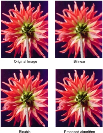
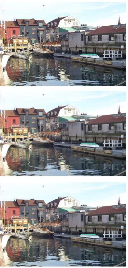
(7) Figure 6 shows a flower test image and its interpolated images produced with different interpolation schemes. To show the differences in detail, Figure 7 presents the enlarged small portions from the original and the interpolated images. A natural scene image containing many high-frequency spatial details and its reconstructed images are shown in Figure 8. Although some highfrequency details are lost in each of the interpolated images, the images produced by the proposed method can better preserve the edge sharpness and color consistency without introducing unpleasant interpolation artifacts.. 9. N.S Jayant and P. Noll, “Digital coding of waveforms: principles and applications to speech and video”, PrenticeHall, 1984. 10. Chang, Ed., "Color Filter Array Recovery Using a Threshold-based Variable Number of Gradients", Proceedings of SPIE, January 1999. 11. Image interpolation web site at Cornell University, http://www.ee.cornell.edu/~splab/interpolation/. 7. CONCLUSION We have presented a new and improved image interpolation method that can adapt to local image structure for constructing high-resolution color images from their down-sampled versions. Our main contributions include using image spatial correlation to form an edge directed interpolator for constructing a highresolution green image plane and exploiting spectral correlation between different color planes to up-sample the red and blue color planes. Both steps involve with the searching for neighboring pixels that possess similar statistical characteristics as the pixel to be interpolated. Simulation results show that the proposed method can generate more visually pleasing images compared to that produced by other commonly used interpolation schemes.. Original Image. Bilinear. Bicubic. Proposed algorithm. 8. REFERENCES 1. R.G. Keys, “Cubic convolution interpolation for digital image processing”, IEEE Trans. Acoust., Speech, Signal Processing, vol. ASSP-29, no. 6, pp. 1153-1160, 1981. 2. Wang, Y. and Mitra, S.K., “Edge Preserved Image Zooming”, Fourth European Signal Processing Conf., Grenoble, France. September 5-8, pp. 1445-1448, 1988. 3. Hong, K.P., Paik, J.K., Kim, H.J. and Lee, C.H., “An EdgePreserving Image Interpolation System for a Digital Camcorder”, IEEE. Trans. Consumer Electronics, Vol. 42, No. 3, pp. 279-284, 1996. 4. Ruderman, D.L. and Bialek, W., “Seeing Beyond the Nyquist Limit”, Neural Computation, Vol. 4, pp. 682-690, 1992. 5. Jensen, K. and Anastassiou, D., “Subpixel Edge Localization and the Interpolation of Still Images”, IEEE Trans. Image Processing, Vol. 4, No. 3, pp. 285-295, 1995. 6. Bayrakeri, S.D. and Mersereau, R.M., “A New Method for Directional Image Interpolation”, Proc. Int. Conf. Acoustics, Speech, Sig. Processing, Vol. 4, pp. 2383-2386, 1995. 7. H.Nicos and N.Anastasios, “Color Image Interpolation for high resolution acquisition and display devices”, IEEE Trans. On Consumer Electronics, Nov 1995. 8. Xin Li and Michael Orchard, “New Edge Directed Interpolation", Int. Conf. On Image Processing, 2000.. Figure 6: Original flower image and its interpolated results.. Original. Bicubic. Bilinear. Proposed algorithm. Figure 7: Portions of original and the interpolated images..

(8) Original. Bilinear. Proposed Algorithm. Figure 8: Original scene image and its interpolated results..

(9)