The Relationship between Volatility and Expected Returns:Some Evidence for Australia

全文

(1)International Journal of Business and Economics, 2011, Vol. 10, No. 1, 27-43. The Relationship between Volatility and Expected Returns: Some Evidence for Australia Ali F. Darrat* College of Business, Louisiana Tech University, Ruston, U.S.A. Bin Li Griffith Business School, Griffith University, Australia Omar Benkato Miller College of Business, Ball State University, U.S.A.. Abstract We explore the intertemporal relation between the conditional mean and the conditional variance of industry portfolio returns and the Fama-French 25 size/book-tomarket portfolio returns using data from Australia. We estimate the portfolio conditional covariance with the market and test whether it can predict the time-variation in the portfolio expected returns. We find strong and consistent evidence of a positive risk aversion relation, implying that the market returns do carry a positive risk premium in the Australian market. Our results suggest that the value factor is relevant for determining the variation of asset returns on both the industry portfolios and the size/book-to-market portfolios. Key words: risk-return trade-offs; volatility models; ICAPM; Australian market JEL classification: G12; G13; C51. 1. Introduction Finance theory postulates a positive relation between risk and expected returns. If investors perceive a given asset to be highly risky they require higher return. This risk-return relation is particularly important for asset valuation since the present values of future cash flows or dividends are calculated by discounting them using the required rate of return. Therefore, correctly accounting for the risk-return relation can provide a better understanding of assets’ required rates of return and the valuation of these assets.. Received February 16, 2011, revised May 21, 2011, accepted May 29, 2011. * Correspondence to: College of Business, Louisiana Tech University, Ruston, LA 71272, U.S.A. E-mail: darrat@cab.latech.edu. The authors wish to thank an anonymous referee of this journal for several useful comments..

(2) 28. International Journal of Business and Economics . The risk of an asset can be measured as the covariance of the asset’s return with the market return in the context of Sharpe’s (1964) capital asset pricing model (CAPM). Asset’s risk can also be measured as the covariance with other common factors related to the investors’ marginal utility in Merton’s (1973) intertemporal capital asset pricing model (ICAPM). If the asset is itself the market portfolio, risk is the conditional variance of the market return. Building upon the ICAPM, Merton (1980) argues that conditional expected excess returns are positively related to the conditional variance. The coefficient of the conditional variance can be interpreted as the relative risk aversion. Theory suggests that the relative risk aversion parameter should be significantly positive as investors require a larger risk premium whenever the stock market becomes riskier. However, available empirical evidence on this contention is largely inconclusive. For example, French et al. (1987), Chou (1988), Bollerslev et al. (1988), Ghysels et al. (2005), Bali and Peng (2006), and Bali (2008) support a statistically significant positive relation. However, Campbell and Hentschel (1992), Chan et al. (1992), and Goyal and Santa-Clara (2003) fail to detect any significant relation. Indeed, results in Campbell (1987), Nelson (1991), Glosten et al. (1993), and Harvey (2001) suggest instead a significantly negative relation. Attempting to explain these conflicting results, Glosten et al. (1993) and Harvey (2001) argue that the relative risk aversion is particularly sensitive to model specifications. Most prior research examines the time series relation between risk and returns using the market portfolio. Yet, Merton’s (1980) hypothesis applies to both individual and portfolio returns. In this paper, we analyze the intertemporal riskreturn relation in the case of Australia using portfolio data that include industry returns and the 25 Fama-French size and book-to-market sorted portfolio returns. Australia has become a major financial center in the Asian Pacific region. As of June 30, 2008, there were 2,226 companies listed on the Australian exchange with market capitalization of AUD 1.29 trillion, making the Australian stock market the eighth largest in the world and second only to Japan in the Asian Pacific region. Previous research on the volatility of the Australian stock market includes Brailsford and Faff (1993), Kearns and Pagan (1993), and Nicholls and Tonuri (1995), who use variants of the GARCH model to examine the time-variation in volatility. In addition, Kearney and Daly (1998) examine possible causes of stock market volatility, while Sault (2005) investigates asset price volatility at the firm and industry levels. However, none of these studies examines the intertemporal riskreturn relation in the Australian market. We explore the intertemporal relation in Australia between the conditional mean and the conditional variance of the industry portfolio returns and the FamaFrench 25 size/book-to-market (Size/BM) portfolios using a variant of the GARCH model proposed by Baba et al. (1991), henceforth the BEKK-GARCH model. We estimate a portfolio’s conditional covariance with the market returns and test whether the conditional covariance helps predict the time-variation in the portfolio expected returns. Our results indicate the presence of a significantly positive relation.

(3) Ali F. Darrat, Bin Li, and Omar Benkato. 29. between asset returns and the market returns in Australia. We further find some evidence linking asset returns to the size and value factors. This paper also contributes to the literature in two additional ways. First, we test the intertemporal risk-return relation in Australia by performing out-of-sample tests. Our results strongly support the positive risk-return relation that some studies document for the US market using portfolio data. Second, this paper represents the first attempt to investigate in the Australian context the risk-return relation using both the industry portfolios and the Fama-French 25 Size/BM portfolios. The rest of the paper is structured as follows. Section 2 discusses the methodology. Section 3 presents the data and the associated summary statistics. Section 4 discusses the empirical results. Section 5 concludes. 2. Methodology In the Merton (1973) setting, the equilibrium risk-returns relation is:. μ = A ∑ +ΩB ,. (1). where μ is the vector of expected excess returns, A measures the representative agent’s relative risk aversion, ∑ is the covariance matrix of excess asset returns with the excess market returns, Ω is the covariance matrix between asset returns and state variables related to investment opportunities, and B is the coefficient matrix denoting the sensitivities of asset returns to state variables. The ICAPM postulates that an asset’s return is determined by its covariance with the market portfolio and with the state variables. Following Bali (2008), we use a two-stage estimation method. In the first stage, we extract the conditional covariance between asset returns and the market returns from a bivariate BEKK-GARCH model.1 In the second stage, we examine the relation between asset returns and the estimated conditional covariance. In the BEKK-GARCH(1,1) model, the mean equations include constants and conditional variances using BEKK-GARCH(1,1) specifications of the forms: Ri , t +1 = a0i + ε 1, t +1 ,. (2). Rm , t +1 = a + ε m , t +1 ,. (3). H t +1 = r0 + r1′H t r1 + r2′ε t ε t′r2 ,. (4). m 0. where Ri , t +1 and Rm , t +1 are excess returns on asset i and the market portfolio at time t + 1 , respectively, and ε t and Vt have the forms: ⎡ε i , t ⎤ εt = ⎢ ⎥ , ⎣⎢ε m , t ⎦⎥. (5).

(4) 30. International Journal of Business and Economics ⎡hii , t him , t ⎤ Ht = ⎢ ⎥, ⎣⎢him , t hmm , t ⎦⎥. (6). where r0 , r1 , and r2 , are 2× 2 matrices. For models with other factors, we estimate the conditional covariance between asset return i and each factor f , denoted hif , using similar specifications as those in (2)–(4) by replacing the terms associated with Rm , t +1 by the terms associated with f m , t +1 . We use the maximum likelihood method to estimate the parameters and extract the conditional covariance of each asset return with the market return. 3. Data and Summary Statistics Our data consist of the monthly industry portfolio returns and the Fama-French 25 Size/BM. The sample spans the period January 1982 to December 2006. All other data come from the Centre of Research in Finance (CRIF) database and the Reserve Bank of Australia.2 The market return data are monthly value weighted returns on the AllOrd market index. To represent the Australian short-term monthly interest rate, we use the 13-week Treasury bill rate. The excess market return is the market return minus the short-term interest rate. Although Campbell (1987) suggests that the level of short-term interest rates may help forecast stock returns, more recent studies like Campbell (1991) and Lettau and Ludvigson (2001) de-trend short-term interest rates due to its non-stationarity. We construct the relative short bill rate as the 13-week Treasury bill rate minus its 12-month backward moving average. The term spread is the difference between the 10-year commonwealth government bond yield and the 13-week Treasury bill rate. Monthly data on dividend yield for the Australian stock market index is available only for recent years in the database. However, Shares magazine (and its predecessors, SXJ) and the Australian Stock Exchange Journal provide average dividend yield and the P/E ratio data over the full estimation period for all traded companies in the Australian Stock Exchange (ASX). We also use the GICS classified monthly industry returns from the CRIF database that contains 25 industry groups.3 We dropped three groups (G8, G9, and G22) due to many missing values, leaving a final sample of 22 industry groups. Recent research on asset pricing models focuses on portfolios sorted on size and book-to-market ratio since, compared to industry or beta portfolios, they reveal more variations in mean returns across firms and across industries (Cochrane, 2006). Fama-French 25 Size/BM portfolios produce size effect, where small size firms have higher average returns than large size firms, and value effect, where firms with high book-to-market ratios have higher average returns than firms with low book-tomarket ratios. Given this data characteristic, we also use Size/BM portfolios to test the risk-return relation in Australia..

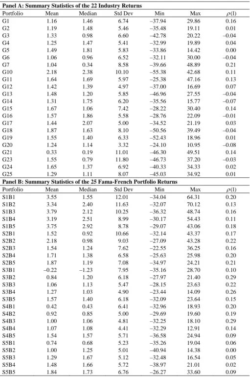
(5) Ali F. Darrat, Bin Li, and Omar Benkato. 31. The Fama-French data are similar to those used by O’Brien (2008), who sorts into the 25 portfolios based on size and book-to-market of all firms traded in the ASX from January 1982 to December 2006 utilizing the procedures of Fama and French (1992, 1993, 1996). O’Brien’s databases include the CRIF monthly stock price file for stock return and size, and his own accounting information compiled from firm’s annual reports for every listed firm. Small minus big (SMB) is constructed as the difference between the average returns on small firm portfolios and the average returns on large firm portfolios, and high minus low (HML) is constructed as the difference between average returns on high book-to-market firm portfolios and the average returns on low book-to-market portfolios. Table 1 gives summary statistics for the portfolio returns. Panel A reports the return summary statistics for the 22 industry portfolios. The mean returns on the industry portfolios (between 0.33% and 2.18%) show less variability than the mean returns on the 25 Size/BM portfolios. The first-order autocorrelation coefficients are low for most industry portfolios. Panel B displays the return statistics of the 25 Size/BM portfolios sorted on the intersections of firm size and book-to-market ratio. S1B1 stands for the portfolio in the smallest size and lowest book-to-market ratio group, while S5B5 stands for the portfolio in the largest size and highest book-tomarket ratio group. The data show that the small size portfolios have higher average returns compared to large size portfolios. The mean monthly returns for the large size portfolios range from 0.74% to 1.84%, while those for the small size portfolios range from 3.19% to 3.79%. In larger size groups (e.g., S5, S4, and S3), the mean returns monotonically increases with the book-to-market ratios in each group. However, this is not the case in smaller size groups (e.g., S1 and S2). The autocorrelation for most portfolio returns are between 10% and 20%. Panel C reports summary statistics for the market return, the risk-free rate, SMB, HML, the detrended risk-free rate, the term spread and the dividend yield. The mean return is 1.20% for the value weighted market portfolio and 0.69% for the risk-free rate. The mean return on SMB and HML is 0.47% and 0.69%, possibly suggesting the presence of value and size premium in the Australian market. We also observe very high autocorrelations of the de-trended risk-free rate, the term spread, and the dividend yield. Table 2 reports the summary statistics for the conditional covariance. We give the sample means, standard deviations, minimum, maximum, first-order autocorrelation, and 12th-order autocorrelation of the estimated conditional series. We also report the unconditional covariance and beta. For both the 22 industry portfolios and the 25 Size/BM portfolios, the unconditional covariance is very close to the mean of the conditional covariance. The standard deviation of the conditional covariance are similar to the mean for both the industry portfolios (Panel A), and the Size/BM portfolios (Panel B). Conditional covariance also exhibits high persistence as measured by the first-order autocorrelation, with most of them being larger than 0.50 for both the industry portfolios and the Size/BM portfolios..

(6) 32. International Journal of Business and Economics Table 1. Summary Statistics for the Portfolio Returns. Panel A: Summary Statistics of the 22 Industry Returns Portfolio Mean Median Std Dev Min G1 1.16 1.46 6.74 –37.94 G2 1.19 1.48 5.46 –35.48 G3 1.33 0.98 6.60 –42.78 G4 1.25 1.47 5.41 –32.99 G5 1.49 1.81 5.83 –33.86 G6 1.06 0.96 6.52 –32.11 G7 1.04 0.34 8.58 –39.66 G10 2.18 2.38 10.10 –55.38 G11 1.64 1.69 5.97 –25.38 G12 1.42 1.39 4.97 –37.00 G13 1.48 1.20 5.85 –46.96 G14 1.31 1.75 6.20 –35.56 G15 1.67 1.06 7.42 –28.22 G16 1.57 1.86 5.58 –28.76 G17 1.44 2.07 5.00 –34.52 G18 1.87 1.63 8.10 –50.56 G19 1.55 1.40 6.33 –52.43 G20 1.24 1.14 3.32 –24.10 G21 0.33 0.19 11.01 –46.30 G23 1.55 0.79 11.80 –46.73 G24 1.65 1.37 6.92 –40.33 G25 1.29 1.11 8.07 –45.03 Panel B: Summary Statistics of the 25 Fama-French Portfolio Returns Portfolio Mean Median Std Dev Min S1B1 3.55 1.55 12.01 –34.04 S1B2 3.34 2.40 11.63 –32.07 S1B3 3.79 2.12 10.25 –36.32 S1B4 3.19 2.51 8.99 –30.17 S1B5 3.75 2.92 8.78 –29.07 S2B1 1.52 0.92 10.66 –32.14 S2B2 2.18 0.98 9.03 –27.09 S2B3 1.54 1.24 7.62 –22.55 S2B4 1.71 1.38 6.58 –25.63 S2B5 1.87 1.19 7.08 –34.97 S3B1 –0.22 –1.23 7.95 –35.16 S3B2 0.84 1.20 6.18 –27.97 S3B3 1.06 1.13 5.47 –28.15 S3B4 1.27 1.03 4.90 –23.44 S3B5 1.57 1.40 6.18 –32.09 S4B1 0.42 0.43 6.41 –32.96 S4B2 0.92 0.85 5.00 –29.69 S4B3 1.00 1.06 4.81 –32.25 S4B4 1.07 1.08 4.41 –32.29 S4B5 1.54 1.57 5.71 –36.58 S5B1 0.74 0.68 5.23 –35.26 S5B2 1.00 1.25 5.01 –40.94 S5B3 1.29 1.67 5.12 –32.48 S5B4 1.48 1.66 5.72 –38.97 S5B5 1.84 1.73 6.76 –26.27. Max 29.86 19.11 20.22 19.89 14.42 30.00 48.89 42.68 47.16 16.69 27.55 15.77 30.40 22.09 21.19 39.49 18.96 10.95 49.51 37.20 34.33 34.92. ρ (1) 0.16 0.01 –0.04 0.04 0.00 –0.04 0.21 0.11 0.13 0.07 –0.04 –0.07 0.14 –0.01 0.03 –0.04 0.01 –0.08 0.14 –0.03 0.02 0.01. Max 64.31 70.12 48.74 54.43 43.06 43.37 43.28 36.25 25.98 24.21 28.70 21.40 23.63 14.09 23.64 18.93 19.60 18.10 12.91 24.94 19.04 14.38 16.54 21.01 33.60. ρ (1) 0.20 0.13 0.16 0.11 0.18 0.17 0.22 0.16 0.20 0.21 0.10 0.29 0.22 0.26 0.15 0.20 0.19 0.29 0.14 0.09 0.06 0.00 0.05 0.02 0.09.

(7) Ali F. Darrat, Bin Li, and Omar Benkato. 33. Panel C: Summary Statistics of the Explanatory Variables. Variables. Mean. RM. Median. 1.20. Std Dev. 1.49. 4.59. Min –39.53. Max. ρ (1). 15.08. 0.01. RF. 0.69. 0.52. 0.33. 0.34. 1.49. 0.98. SMB HML. 0.47 0.69. 0.08 0.66. 5.48 3.36. –19.37 –12.40. 25.16 13.85. 0.25 0.11. RREL. –0.01. 0.00. 0.12. –0.42. 0.37. 0.88. TRM 0.05 0.07 0.14 –0.33 0.38 0.92 DP 4.05 3.76 0.94 2.53 7.02 1.00 Notes: Figures are in percentages except for ρ (1) . Panel A reports the summary statistics of the monthly industry portfolio returns. See endnote 4 for the 22 industry group categorizations. Panel B reports the summary statistics of the Fama-French 25 size/book-to-market portfolio returns sorted on the interaction of firm size and book-to-market ratio. “S1B1” denotes the portfolio in smallest size and lowest book-tomarket ratio group, while “S5B5” denotes the portfolio in the largest size and highest book-to-market ratio group. Panel C reports the summary statistics of the explanatory variables. RM is the return on the value-weighted market indices. RF is the return on the risk-free asset represented by the 13-week Treasury bill rate. SMB is the returns on the small group minus the return on the large group, and HML is the returns on the highest book-to-market ratio group minus the return on the lowest book-to-market ratio group. RREL is the relative risk-free rate. TRM is the term spread between the ten-year government bond yield and the 13-week Treasury bill rate. DP is the 12-month moving average market dividend yield. Table 2. Summary Statistics for the Conditional Covariance Estimates Panel A: The 22 Industry Portfolios. Industry G1 G2 G3 G4 G5 G6 G7 G10 G11 G12 G13 G14 G15 G16 G17 G18 G19 G20 G21 G23 G24 G25. Uncon (×100). Mean (×100). 0.21 0.21 0.25 0.20 0.19 0.12 0.16 0.30 0.15 0.17 0.18 0.20 0.16 0.18 0.17 0.24 0.23 0.10 0.24 0.27 0.18 0.26. 0.19 0.24 0.28 0.19 0.21 0.12 0.16 0.28 0.15 0.19 0.16 0.20 0.18 0.16 0.18 0.26 0.23 0.10 0.27 0.21 0.17 0.31. StdDev (×100) 0.12 0.32 0.30 0.11 0.27 0.12 0.14 0.29 0.27 0.29 0.16 0.26 0.30 0.10 0.15 0.32 0.22 0.19 0.33 0.21 0.15 0.48. Min (×100) –0.02 0.07 0.07 0.08 0.06 0.00 0.00 0.00 –0.36 0.02 –0.02 –0.80 0.03 0.06 0.06 0.02 0.04 0.03 –0.16 –0.03 0.02 0.01. Max (×100) 0.50 3.15 2.74 0.88 2.72 0.93 1.14 2.35 3.23 2.46 1.14 2.32 4.56 0.66 1.79 2.89 1.65 3.16 3.43 1.42 1.00 3.31. ρ (1) 0.98 0.85 0.87 0.96 0.83 0.89 0.90 0.85 0.79 0.90 0.97 0.69 0.42 0.92 0.71 0.49 0.92 0.13 0.66 0.56 0.63 0.97. ρ (12) 0.55 0.14 0.16 0.18 0.17 0.26 0.17 0.18 0.10 0.34 0.15 0.10 0.05 0.65 0.34 0.28 0.16 –0.02 0.08 0.49 0.74 0.18.

(8) International Journal of Business and Economics . 34. Panel B: The Fama-French 25 Size/BM Portfolios. Portfolio. Uncon (×100). Mean (×100). StdDev (×100). Min (×100). Max (×100). ρ (1). ρ (12). S1B1 0.22 0.25 0.27 0.00 2.51 0.81 0.24 S1B2 0.21 0.22 0.26 –0.20 1.59 0.87 0.06 S1B3 0.20 0.22 0.22 –0.03 1.45 0.93 0.18 S1B4 0.17 0.17 0.17 –0.28 1.12 0.87 0.16 S1B5 0.19 0.23 0.30 –0.16 2.65 0.90 0.13 S2B1 0.25 0.25 0.20 –0.06 1.42 0.90 0.24 S2B2 0.21 0.24 0.26 0.05 2.04 0.91 0.15 S2B3 0.17 0.20 0.20 –0.08 1.34 0.92 0.15 S2B4 0.15 0.15 0.12 –0.64 0.77 0.64 0.16 S2B5 0.19 0.18 0.12 0.04 0.72 0.73 0.30 S3B1 0.23 0.25 0.26 0.06 2.56 0.85 0.19 S3B2 0.17 0.16 0.16 –0.66 1.91 0.52 0.00 S3B3 0.15 0.16 0.17 –0.12 1.82 0.73 0.08 S3B4 0.14 0.16 0.23 0.00 3.06 0.56 0.17 S3B5 0.18 0.19 0.26 0.06 2.92 0.76 0.09 S4B1 0.21 0.23 0.27 0.08 2.96 0.80 0.13 S4B2 0.17 0.17 0.28 –0.17 3.94 0.47 0.07 S4B3 0.17 0.15 0.18 0.06 2.35 0.56 0.05 S4B4 0.16 0.15 0.10 0.04 0.66 0.45 0.14 S4B5 0.17 0.15 0.17 –0.02 1.22 0.87 –0.07 S5B1 0.21 0.21 0.21 0.04 1.53 0.94 0.40 S5B2 0.21 0.20 0.13 0.05 1.09 0.74 0.46 S5B3 0.21 0.23 0.24 0.05 1.83 0.91 0.30 S5B4 0.20 0.24 0.28 –0.02 2.30 0.89 0.22 S5B5 0.18 0.19 0.23 –0.24 2.87 0.62 –0.03 Notes: The table reports summary statistics for the conditional covariance and conditional beta estimates between excess asset returns and the excess market returns. Panel A reports the results for the 22 industry portfolios, while Panel B does the same for the 25 Fama-French portfolios sorted on size and book-tomarket ratio. In each panel, the unconditional covariance (Uncon), mean, standard deviation, minimum, maximum, and first- ( ρ (1) ) and 12th-order ( ρ (12) ) coefficients of the conditional covariance are presented. See also notes to Table 1.. 4. Empirical Results We use Hansen’s (1982) general method of moments (GMM) to estimate the risk-return relation using the conditional covariance extracted from a bivariate BEKK-GARCH(1,1) as given in (2)–(6). The moment restriction for asset i is:. gi , t. ⎡ ⎤ Ri , t +1 − Ci − γhim , t +1 − B′h if , t +1 ⎢ ⎥ = ⎢ (Ri , t +1 − Ci − γhim , t +1 − B′h if , t +1 )him , t +1 ⎥ = 0 , i = 1,K , N , ⎢(R − C − γh ⎥ ′ ) i im , t +1 − B h if , t +1 ⊗ h im , t +1 ⎦ ⎣ i , t +1. (7).

(9) Ali F. Darrat, Bin Li, and Omar Benkato. 35. where B is a vector of loadings on the k factors, h if , t +1 is the vector of the conditional covariance between excess asset returns and other factors including SMB and HML, and ⊗ denotes a Kronecker product. N = 22 is the number of industry portfolios, N = 25 for the Fama-French portfolios sorted on size and bookto-market ratio, and N = 47 for the combined portfolios system. Following Bali (2008), we restrict the relative risk aversion to be the same for each asset in order to enhance the statistical power of the estimates and provide consistent slope estimates. Specifically, we restrict the slope estimate γ and/or B to be the same across all assets but allow abnormal returns Ci to differ in each asset. We estimate the system of equations by an iterated GMM where the estimator weighting matrix is continuously updated until convergence.4 4.1 The Conditional Covariance with the Market Returns We begin by examining the relation between excess asset returns and their conditional covariance with the excess market returns. Panel A of Table 3 uses the GMM method on the system of which the moment restriction for asset i is: ⎡ Ri , t +1 − Ci − γhim , t +1 ⎤ gi, t = ⎢ ⎥ = 0 , i = 1,K , N . ⎣⎢(Ri , t +1 − Ci − γhim , t +1 )him , t +1 ⎦⎥. (8). For example, the system for the 22 industry portfolios has 44 moment restrictions with 23 parameters to be estimated. Thus, the system is over-identified with 21 degrees of freedom. The GMM slope estimate ( γ ) in Panel A is the coefficient of relative risk aversion of the representative market investor. We also report beneath the slope estimates the Newey-West (1987) statistics with four lags to correct for residual autocorrelation (higher lags give similar results). The relative risk aversion estimate is 1.29 for the 22 industry portfolios and 2.13 for the 25 Size/BM portfolios; both of these estimates are highly significant (t-statistics are 4.46 and 5.37, respectively). The combined industry and Size/BM portfolios system yields similar results ( γ = 2.48 and t-statistic=10.26). Taken together, these results consistently suggest the presence of a significantly positive relation between asset return and the market risk in Australia. Moreover, the coefficients of relative risk aversion of about 1 to 3 appear economically reasonable and of similar magnitudes to those reported by Bali (2008) for the US market. One might question the sensitivity of our results to possible structural breaks. In particular, the first part of our sample (1982–1992) witnessed several important developments that may have caused structural breaks, including the floating of the Australian dollar in 1983, the deregulation of the banking industry during 1983– 1985, the stock market crash in October 1987, and the recession of 1989–1992. Merging this apparently tense period with the rest of the data may have smoothed out the data and masked instability evidence in the full sample estimates. However, it is reassuring that our main conclusion derived in the full sample regarding the.

(10) International Journal of Business and Economics . 36. significantly positive risk-return relation in Australia remains intact in the first turbulent period (see Panel A of Table 3).5 Table 3. The Intertemporal Risk/Returns Relation Panel A. Portfolios 22 Industry Portfolios. Full Sample 1.29*** (4.46). 25 Size/BM Portfolios. 2.13*** (5.37) 1.82***. Both. 1982:1–1992:12 1.52*** (4.87) 2.80*** (4.90). (10.26) Panel B. Full Sample Market Portfolios. 1982:1–1994:12. –0.38. –0.31. (–0.57). (–0.51). Notes: Panel A displays the coefficient estimates of relative risk aversion ( γ ) from the model moment conditions. The system is estimated by iterated GMM with the constraints that the slope estimates γ be the same for all assets. The heteroskedasticity- and autocorrelation-consistent t-statistics (computed using the Newey-West (1987) standard errors with 4-lag corrections) are in parentheses below the slope estimates. The results for the turbulent period (January 1982–December 1992) are also presented. Panel B estimates equation (9). ***, **, and * denote significance at the 1%, 5%, and 10% levels, respectively.. To what extent are our results sensitive to using aggregate market indices? To check this aspect, we estimate the Australian risk-return relation on the basis of the aggregate market index using the equation:. Rm , t +1 = C + γhmm , t +1 + ε i , t +1 ,. (9). where hmm , t +1 is the market conditional volatility extracted from a GARCH(1,1) model for the single excess market return series. Panel B of Table 3 reports the results. The estimated coefficient of the relative risk aversion is statistically insignificant both in the full sample and also in the first (turbulent) sub-period. This illustrates the failure of using single market return series for identifying risk-return relations.6 The strong positive risk-return relation we find from the Australian portfolio data lends support to Bali’s (2008) contention that the use of a large crosssection of return series, while constraining them to share the same slope, provides cross-sectional consistency in pricing all portfolios according to the same risk-return relation. Such a practice enhances the statistical power for detecting credible and economically sensible risk-return coefficients. 4.2 Relation with the Conditional Covariance and SMB/HML Factors The results in the previous section suggest that there is a significantly positive intertemporal relation between asset return and the market risk in Australia. As.

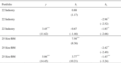
(11) Ali F. Darrat, Bin Li, and Omar Benkato. 37. Fama and French (1992, 1993, 1996) and Cochrane (2005, p. 160) argue, state variables such as SMB and HML can predict shifts in future investment opportunities and are thus important factors in the Merton ICAPM. In this section, we examine the intertemporal relation between asset return and its covariance with the SMB and HML factors in addition to the market factor. The GMM system is represented in (7), where h if , t +1 is a vector of the estimated conditional covariance between excess asset returns and the SMB factor ( his , t +1 ) and the estimated conditional covariance between excess asset returns and the HML factor ( hih , t +1 ). We extract his , t +1 and hih , t +1 from the bivariate GARCH(1,1) model using similar specifications as those under equations (2)–(6) by replacing the terms associated with the market returns by those associated with SMB and HML, respectively. Table 4 reports the estimation results we obtained from the GMM system (7). To preserve cross-sectional consistency, we constrain the slope coefficients for the market risk, γ , for the SMB factor, Bs , and for the HML factor, Bh , to be the same in all moment restrictions. We begin by estimating the SMB and HML. The beta for the SMB factor is positive only for the 25 Size/BM portfolios (coefficient 7.50, tstatistic=8.36), implying that portfolios which have higher covariance with the size factor tend to have higher expected returns. However, the SMB beta for the industry portfolio is insignificant at conventional levels. On the other hand, the beta estimates for the HML factor in the Fama-French three-factor model reverses sign (becoming negative) and are significant at conventional levels. For example, in the 25 Size/BM portfolios, the beta estimate of the HML factor is –2.42 with a t-statistic of –2.49. Nevertheless, for both sets of portfolios, the estimates of the market risk aversion remain positive and highly significant (i.e., for the 22 industry portfolios, γ = 3.45 with t-statistic=11.62). In sum, our finding of a robust and positive risk-return relation in Australia persists even after accounting for the size and value factors. 4.3 Relation with the Macroeconomic Variables A number of macroeconomic variables may also predict future shifts in investment opportunities, thus representing risk factors in the ICAPM. The usefulness of the relative Treasury security rate for predicting US stock returns are documented in Campbell (1991) and Hodrick (1992). Fama and French (1989) underscore the predictive power of the term spread. Market dividend yields may also have some predictive power (Shiller, 1984; Campbell and Shiller, 1988; and Fama and French, 1988). Consequently, we examine in this section the possible sensitivity of the risk-return relation in Australia to three key macroeconomic variables, namely, the relative Treasury bill rate ( RRELt ), changes in the term spread ( TRM t ), and changes in the dividend-price ratio ( DPt )..

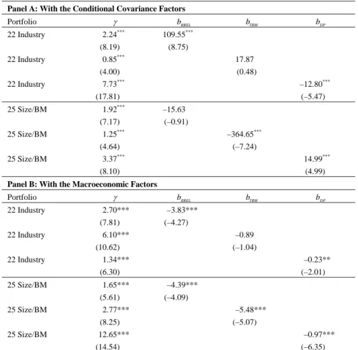
(12) International Journal of Business and Economics . 38. Table 4. The Conditional Covariance with the SMB, HML and Idiosyncratic Volatility. Portfolio. γ. bs. 22 Industry. bh. 0.88 (1.17) –2.96**. 22 Industry. (–2.52) 22 Industry. 3.45. ***. (11.62). –1.83**. –0.67 (–1.46). (–2.66). ***. 25 Size/BM. 7.50. (8.36) –2.42**. 25 Size/BM. (–2.49) 25 Size/BM. 5.06***. 3.77***. –1.43***. (14.45) (10.21) (–3.24) Notes: This table reports the estimated coefficient of relative risk aversion ( γ ) and/or the betas for SMB, HML, and idiosyncratic volatility factor from the model moment conditions. The system is estimated by iterated GMM with the constraint that the slope estimates γ and B be the same for all assets. See also notes to Table 3.. Panel A of Table 5 gives the loading estimates on the conditional covariance factors with the three macro variables. Following Bali (2008), these variables enter the model with one lag (the main evidence of a positive risk-return relation between asset returns and the market factor is robust to using different lags). We extract the conditional covariance between excess asset returns and the macro variables from the bivariate BEKK-GARCH(1,1) model. As before, we restrict the slope estimate γ and Bx to be the same for all equations. The results in Panel A indicate that the risk aversion estimates for market factor do not noticeably change (compared to the estimate for the combined SMB/HML factor in Table 4). That is, these estimates remain positive and highly significant in the presence of these macro variables. The beta estimate for the relative Treasury bill rate are positive for the industry portfolios, suggesting that the covariance between asset excess returns with the short interest rate provides an additional risk premium necessary for investors to hold the asset. On the other hand, the beta estimate for the term spread is statistically negative for the Size/BM portfolios, indicating any downward movement in this variable would predict favorable shifts in the investment opportunity. The results further indicate that the dividend-price ratio bears significantly negative coefficients for the industry portfolios but has significant and positive coefficients for the Size/BM portfolios..

(13) Ali F. Darrat, Bin Li, and Omar Benkato. 39. Table 5. Relations with the Macroeconomic Variables Panel A: With the Conditional Covariance Factors Portfolio 22 Industry. γ 2.24*** (8.19). bRREL. bTRM. (8.75). 22 Industry. 0.85***. 17.87 (0.48). 22 Industry. (4.00) 7.73***. –12.80***. (17.81). (–5.47). 25 Size/BM. 1.92***. –15.63. (7.17) 1.25***. (–0.91). 25 Size/BM. –364.65*** (–7.24). (4.64) 25 Size/BM. bDP. 109.55***. 3.37***. 14.99*** (4.99). (8.10). Panel B: With the Macroeconomic Factors. γ. bRREL. 22 Industry. 2.70***. –3.83***. 22 Industry. (7.81) 6.10***. Portfolio. 22 Industry. 1.65***. 25 Size/BM. (5.61) 2.77***. bDP. (–4.27) –0.89. (10.62) 1.34*** (6.30). 25 Size/BM. bTRM. (–1.04) –0.23** (–2.01) –4.39*** (–4.09) –5.48***. (8.25) (–5.07) 25 Size/BM 12.65*** –0.97*** (14.54) (–6.35) Notes: This table presents the estimates of the loadings on three macroeconomic variables from the model moment conditions. The system is estimated by GMM with the constraints that the slope γ and Bx be the same for all the equations. Panel A uses the conditional covariance factors. hix , t +1 is the estimated conditional covariance between excess asset returns and the relative Treasury Bill rate ( RRELt ), changes in the term spread ( TRM t ), and changes in the dividend-price ratio ( DPt ). The hix , t +1 are extracted from a bivariate BEKK-GARCH(1,1) model. Panel B incorporates macroeconomic variables.. Next, we directly include the macroeconomic variables into the GMM system, yielding an error term of the form: g i , t +1 = Ri , t +1 − Ci − γhim , t +1 − BX t , i = 1,K , N ,. (10). where X t contains the relative Treasury bill rate, the term spread, the dividend-price ratio and the lagged excess market return. Panel B in Table 5 reports the results, which indicate that adding macroeconomic variables directly into the GMM system.

(14) 40. International Journal of Business and Economics . do not alter the estimates of market risk aversion either. Again, this suggests that the conditional covariance with the market returns do matter for asset pricing in that when an asset’s conditional covariance with the market portfolio rises, the expected return on the asset will also rise. The coefficients γ are positive and large (ranging between 2 and 13) and statistically significant. The market dividend yield remains significant in both portfolios. The negative sign of the beta estimate suggests that a higher dividend yield in any given month causes a lower expected excess portfolio return in the following month. One major difference in the results between Panels A and B of Table 5 is that beta estimates on the relative Treasury bill rate in Panel B are statistically significant and negative. This negative sign suggests that rising short-term interest rates predict lower one-month ahead excess returns. This finding is consistent with the evidence reported by Ang and Bekaert (2007) and Bali (2008) that short-term interest rates are negatively associated with low excess returns at short horizons. 5. Conclusion. We investigate the intertemporal relation between the conditional mean and the conditional variance in Australia using a bivariate BEKK-GARCH framework. Our sample consists of two sets of portfolios: 22 industry portfolio returns and the FamaFrench 25 Size/BM portfolios sorted on size and book-to-market value. We test whether the estimated portfolio’s conditional covariance matters for predicting the time-variation in the portfolios’ expected returns in Australia. The results robustly support the presence of a significantly positive relation between asset returns and the market returns for both set of portfolios. We further explore asset returns with the SMB (size) and HML (value) factors, and the results persist in their support for a statistically positive risk-return relation even after controlling for the size and value factors. There is also some evidence of a positive relationship between returns on Size/BM portfolios with the size factor but a negative relationship between returns on both portfolios and the value factor. In addition, we examine the sensitivity of our results to incorporating three key macroeconomic variables (the relative Treasury bill rate, the term spread, and the market dividends) in the GMM system. Again, the results continue to reveal highly significant market risk aversion estimates even after accounting for these macroeconomic variables. The significantly positive risk aversion we find in the Australian market implies that market returns do carry a positive risk premium. When a stock’s conditional covariance with the market returns is low, the expected return required on this stock will also be low because investors prefer stocks that do well when the expected market returns fall. This empirical finding has practical implications for asset pricing. Investors price an asset in such a way that its mean excess return must be proportional to its conditional covariance with the market returns. Regulators in the public utility industry, for example, can also use this risk-return relation to obtain the proper discount rate for determining the maximum price these firms can charge..

(15) Ali F. Darrat, Bin Li, and Omar Benkato. 41. Notes 1.. One advantage of the BEKK formulation over standard bivariate GARCH models is that the BEKK formulation imposes positive definiteness on the variance matrix.. 2.. We thank Michael O’Brien for supplying us with the Fama-French 25 portfolio data.. 3.. The categories are: Energy (G1), Material (excluding Metals & Mining) (G2), Metals & Mining (G3), Capital Goods (G4), Commercial Services & Supplies (G5), Transportation (G6), Automobile & Components (G7), Consumer Durables & Apparel (G8), Consumer Services (G9), Media (G10), Retailing (G11), Food & Staples Retailing, Household & Personal Products (G12), Food Beverage & Tobacco (G13), Health Care Equipment & Service (G14), Pharmaceuticals & Biotechnology & Life Sciences (G15), Banks (G16), Diversified Financials (G17), Insurance (G18), Real Estate (excluding REITs) (G19), and Real Estate Investment Trusts (G20), Software & Service (G21), Technology Hardware & Equipment (G22), Telecom Services (G23), Utilities (G24), and GICS pending (G25).. 4.. Ferson and Foerster (1994) argue that the iterated GMM performs better than the two-stage GMM in small samples.. 5.. Results from the Chow test corroborate the structural stability of the estimates. Details are available upon request.. 6.. The inability of single market return series to reveal significant risk-return relations is not confined to using the GARCH(1,1) specification. Results (available upon request) from using both the Nelson (1991) EGARCH and the Glosten et al. (1993) GARCH models fail to produce reliable risk-return relations.. References. Ang, A. and G. Bekaert, (2007), “Stock Return Predictability: Is It There?” Review of Financial Studies, 20, 651-707. Baba, Y., R. F. Engle, D. F. Kraft, and K. F. Kroner, (1991), “Multivariate Simultaneous Generalized ARCH,” Working Paper, University of California, San Diego. Bali, T. G., (2008), “The Intertemporal Relation between Expected Returns and Risk,” Journal of Financial Economics, 87, 101-131. Bali, T. G. and L. Peng, (2006), “Is There a Risk-Return Trade-off? Evidence from High-Frequency Data,” Journal of Applied Econometrics, 21, 1169-1198. Bollerslev, T., R. F. Engle, and J. M. Wooldridge, (1988), “A Capital Asset Pricing Model with Time-Varying Covariances,” Journal of Political Economy, 96, 116-131. Brailsford, T. J. and R. W. Faff, (1993), “Modelling Australian Stock Market Volatility,” Australian Journal of Management, 18, 109-132. Campbell, J. Y., (1987), “Stock Returns and the Term Structure,” Journal of Financial Economics, 18, 373-399. Campbell, J. Y., (1991), “A Variance Decomposition for Stock Returns,” Economic Journal, 101, 157-179..

(16) 42. International Journal of Business and Economics . Campbell, J. Y. and L. Hentschel, (1992), “No News is Good News: An Asymmetric Model of Changing Volatility in Stock Returns,” Journal of Financial Economics, 31, 281-318. Campbell, J. Y. and R. Shiller, (1988), “The Dividend-Price Ratio and Expectations of Future Dividends and Discount Factors,” Review of Financial Studies, 1, 195-228. Chan, K. C., G. A. Karolyi, and R. M. Stulz, (1992), “Global Financial Markets and the Risk Premium on U.S. Equity,” Journal of Financial Economics, 32, 137167. Chou, R. Y., (1988), “Volatility Persistence and Stock Valuations: Some Empirical Evidence Using GARCH,” Journal of Applied Econometrics, 3, 279-294. Cochrane, J. H., (2005), Asset Pricing, New Jersey: Princeton University. Cochrane, J. H., (2006), “Financial Markets and the Real Economy,” in International Library of Critical Writings in Financial Economics, J. H. Cochrane ed., London: Edward Elgar. Vol.18. Fama, E. F. and K. R. French, (1988), “Dividend Yields and Expected Stock Returns,” Journal of Financial Economics, 22, 3-25. Fama, E. F. and K. R. French, (1989), “Business Conditions and Expected Returns on Stocks and Bonds,” Journal of Financial Economics, 25, 23-49. Fama, E. F. and K. R. French, (1992), “The Cross-Section of Expected Stock Returns,” Journal of Finance, 47, 427-465. Fama, E. F. and K. R. French, (1993), “Common Risk Factors in the Returns on Stocks and Bonds,” Journal of Financial Economics, 33, 3-56. Fama, E. F. and K. R. French, (1996), “Multifactor Explanations of Asset Pricing Anomalies,” Journal of Finance, 51, 55-84. Ferson, W. E. and S. R. Foerster, (1994), “Finite Sample Properties of the Generalized Method of Moments in Tests of Conditional Asset Pricing Models,” Journal of Financial Economics, 36, 29-55. French, K. R., G. W. Schwert, and R. F. Stambaugh, (1987), “Expected Stock Returns and Volatility,” Journal of Financial Economics, 19, 3-29. Ghysels, E., P. Santa-Clara, and R. Valkanov, (2005), “There is a Risk-Return Trade-off After All,” Journal of Financial Economics, 76, 509-548. Glosten, L. R., R. Jagannathan, and D. E. Runkle, (1993), “On the Relation between the Expected Value and the Volatility of the Nominal Excess Return on Stocks,” Journal of Finance, 48, 1779-1801. Goyal, A. and P. Santa-Clara, (2003), “Idiosyncratic Risk Matters!” Journal of Finance, 58, 975-1007. Hansen, L. P., (1982), “Large Sample Properties of Generalized Method of Moments Estimators,” Econometrica, 50, 1029-1054. Harvey, C. R., (2001), “The Specification of Conditional Expectations,” Journal of Empirical Finance, 8, 573-637. Hodrick, R., (1992), “Dividend Yields and Expected Stock Returns: Alternative Procedures for Inference and Measurement,” Review of Financial Studies, 5, 357-386..

(17) Ali F. Darrat, Bin Li, and Omar Benkato. 43. Kearney, C. and K. Daly, (1998), “The Causes of Stock Market Volatility in Australia,” Applied Financial Economics, 8, 597-605. Kearns, P. and A. Pagan, (1993), “Australian Stock Market Volatility: 1875–1987,” Economic Record, 69, 163-178. Lettau, M. and S. Ludvigson, (2001), “Consumption, Aggregate Wealth and Expected Stock Returns,” Journal of Finance, 56, 815-849. Merton, R. C., (1973), “An Intertemporal Capital Asset Pricing Model,” Econometrica, 41, 867-887. Merton, R. C., (1980), “On Estimating the Expected Return on the Market: An Exploratory Investigation,” Journal of Financial Economics, 8, 323-361. Nelson, D. B., (1991), “Conditional Heteroskedasticity in Asset Returns: A New Approach,” Econometrica, 59, 347-370. Newey, W. K. and K. D. West, (1987), “Hypothesis Testing with Efficient Method of Moments Estimation,” International Economic Review, 28, 777-787. Nicholls, D. and D. Tonuri, (1995), “Modelling Stock Market Volatility in Australia,” Journal of Business Finance and Accounting, 22, 377-396. O’Brien, M., (2008), “Size, Book to Market and Momentum Effects in the Australian Stock Market,” PhD Thesis, School of Business, The University of Queensland. Sault, S., (2005), “Movements in Australian Stock Volatility: A Disaggregated Approach,” Australian Journal of Management, 30, 303-320. Sharpe, W. F., (1964), “Capital Asset Prices: A Theory of Market Equilibrium under Conditions of Risk,” Journal of Finance, 19, 425-442. Shiller, R., (1984), “Stock Prices and Social Dynamics,” Brookings Papers on Economic Activity, 2, 457-498..

(18)