Efficient Computation of the Eigensubspace for Array Signal Processing

(1)

Efficient computation of

the

eigensubspace for array

signal processing

>

C.-C.Lee and J.-H.Lee

Abstract: The authors present an efficient technique for computing the eigensubspace spanned by a received array data vector. First, the sensor array is partitioned into several subarrays without overlapped sensors. The basis matrix for the signal subspace of each subarray is computed. Using these basis matrices, an additional subarray is constructed and the basis matrix for the corresponding signal subspace is also computed. By using these subarray basis matrices, the basis matrix for the signal subspace of the original sensor array can be computed with reduced computing cost. The statistical performance and computational complexity for adaptive beamforming and for bearing estimation using the proposed technique are evaluated. The theoretical results are confirmed and illustrated by simulation results.

1 Introduction

Adaptive array signal processing based on the eigenspace- based (ESB) techniques has been widely considered in bearing estimation [ 1, 21 and adaptive beamforming [3-51. Using eigenvalue decomposition (EVD) to eigendecom- pose the observation vector space into a signal subspace and a noise subspace is inevitably required when employing the ESB techniques. However, repeatedly updating the data correlation matrix and, hence, its eigen-decomposition to cope with changing conditions in signal or environment makes the computing cost huge.

Recently, many algorithms have been presented in [6- 131 for alleviating the above difficulty. In [6, 71, the subspace computation problem was formulated as a constrained optimisation problem to be solved for mini- mising the required computing cost. The algorithms of [8- 111 adopt the rank-one update of the data correlation matrix at each sampling time. As a result, the subspaces must be updated when receiving one more data snapshot. As to the two algorithms proposed by [12, 131, the subspaces are computed based on partitioning the original linear array into some specified subarrays. However, the principal hypothesis of unambiguity in developing these two algorithms may not be valid for an array with arbitrary configuration. Unfortunately, to determine whether an array with an arbitrary configuration is unambiguous or not is a very difficult task. Moreover, the effectiveness of these two algorithms cannot be guaranteed when the number of signal sources is overestimated.

In this paper, we develop a technique for efficiently computing the subspaces when processing the data received by an array with arbitrary configuration. Based on the partition of the original array into several nonover- 0 E E , 1999

IEE Proceedings online no. 19990512 DOI; 10.1049hp-rsn: 199905 12

Paper first received 19th August 1997 and in final revised form 4th December 1998

The authors are with the Department of Electrical Engineering, National Taiwan University, Taipei 106, Taiwan

ZEE Proc-Radar; Sonar Navig., Vol. f46, No. 5, October 1999

lapped subarrays, it is shown that the array signal subspace is included in a subspace which is constructed from the subarray signal subspaces. From the basis matrices which span the subarray signal subspaces, we construct an additional subarray by appropriately selecting the array sensors and compute its signal subspace. Using the obtained subarray signal subspaces, the array signal subspace can be computed with much less computing cost as compared to conventional techniques. Moreover, the proposed technique possesses the advantages of the algorithms presented by [12, 131 but eliminates their disadvantages of requiring unambiguity in array configuration. The statistical performance and computing cost of applying the proposed technique to bearing estimation and to adaptive beamforming are also evaluated. The experimental results of using the proposed technique confirm the theoretical work.

2 Array processing based on eigensubspace concept

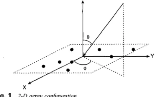
Consider an array with arbitrary configuration and A4 array sensors located on the X-Y plane as shown in Fig. 1. Assume that P ( P < M ) narrowband signal sources are impinging on the array from P distinct direction angles ( 0 ,

bi)

for i = 1,2, . .

.

, P, where

Bi

and

bi

are the elevation and azimuth angles of the ith signal source, respectively. Let a,(@,

4)

be the response of the mth sensor to a signal

J

X

Fig. 1 2 - 0 array Configuration

(2)

source with unit amplitude and direction angle

(e,

4).

Then, the received data of the mth sensor is given by

P

where the uncorrelated signal sources s,(t) have powers equal to n,, i = 1, 2 , .

. .

, P: n,(t) is the received additive white sensor noise with mean zero and equal variance n,. That is, the noise is uncorrelated from sensor to sensor and with the signal. The corresponding data vector Z(t) = [z, (t), z2(t), . . . , zM(t)lT received by the array is then given by

P

=

Em,,

4,>s,(t>

+

N ( t ) = AsSW

+

N ( t ) (2)

41) = [a,(@,

4,))

a2(Qr, 41))

. .

. >

ad&,

4 J T >

the signal

1=1

where the response vector of the ith signal is A(O,, vector is S(t) = [sl(t), s2(t),

.

. . , sp(t)lT, the noise vector is N(t) = [nl(t), n2(t),

.

. ,

n&t)lT, and the array response matrix of all signal sources is A s = [ A ( @ , ,

4 , )

4 8 2 , 4 2 )

.

. .

A(Op,

4p)].

The superscript '7" denotes the transpose operation. The ensemble correlation matrix of Z(t) is given by

R = E { Z ( t ) Z ( t ) H ) = A , F V , A t

+

n,IM (3) where the superscript 'H' denotes the complex conjugate transpose. Fs=E{S(t)S(t)H} =diag{nl, n2,.

.

. , n p } has rank P < M and I, is the A4 x M identity matrix. From the EVD of eqn. 3, we have

M

R = A m e m 4 = E,A,E?

+

E,A,E$ (4)

where A I

2 . .

. 2 A p > Apt =

. .

. = ;IM= n, are the eigen- values and e, is the eigenvector associated with

A,,

The basismatrixEs=[el e2

...

eP]andEN=[ep+, ep+ 2 . . . eM]

both are orthogonal and span the signal subspace (SS) and

the noise subspace (NS) of the array, respectively. The (M-P) x (M-P) diagonal matrix AN = n, I,-p. Many ESB techniques employing the basis matrices Es and EN to deal with the problem of bearing estimation and adaptive beamforming have demonstrated the advantage of better performance over conventional techniques. However, performing the EVD of eqn. 3 requires about 12M3 complex multiplications (CM) [ 151.

m= I

P x P diagonal matrix A , diag{l,, A 2 , . . . , 1,) and the

3 Proposed technique

Let the original M-element array be partitioned into K nonoverlapped subarrays. Let the kth subarray have h f k

sensor elements selected from the original array in such a manner that the data vector &(t) received by this subarray is given by

Zk(t) = JkZ(t) = ASkS(t)

+

Nk(t) (5) where the Mk x M matrix Jk denotes the row selecting matrix containing the appropriate rows of the M x M identity matrix. Ask = Jk A s and Nk(t) = Jk N(t) represents the corresponding response matrix and noise vector for the kth subarray, respectively. Based on eqn. 5 , we note that Jk JT = 0 for

k

#

i, Jk J i = IMk, and Xf=l kt,, = M since the K subarrays do not overlap. Assume that the basis matrices of the SS and NS spanned by &(t) are designated as Gsk and 236

GNk which have Sizes M k X Pk and Mk X (Mk-pk), respec-

tively, where Pk 5 Mk. Then, we have

= range{^^^), and GZkAsk =

o

(6) From eqn. 6, it follows that

Lemma 1: range { J l GNk} S range {As}', where range { A S } l is the complement of range { A s } .

Lemma 1 shows that the vectors o f J l GNk are contained in range { A i } . Next, we construct two full rank matrices as follows:

C N = [JTG,,, J,TG,,, .

. .

, J ~ G N K ] , and c s = [ J ~ G v , ~ 3 J,TGs22 . . ., J ~ G s K I

From Lemma 1, we note that range { C N } Grange {AS}'-. Accordingly, range { A , } C range {Cs} since C, is the basis matrix of range {C,}'. This reveals that a basis matrix for range { A s } can be found from C, with signifi- cantly reduced computing cost. Assume that Gsk has rank equal to

Pk.

Then, Gsk contains a set of Pk rows which are linearly independent. Let Hk be the Pk x Mk row selecting matrix which selects the Pk linearly independent rows from Gsk. A row selecting matrix H based on Jk and Hk is constructed as follows:

H = [(HI J I ) ~ , ( H Z J , ) ~ , . .

.

> ( H K J K ) T I T (8) Using eqn. 8, a data vector with length

is then formed as follows:

i ( t ) = H Z ( t ) =

A&)

+

N(t),

(9)

ks=HA-s and #(t)=HN(t). The SS s p a y e d by z(t) is range { A s } . It is also easy to show that As and As have the same rank because Hk selects the linearly independent rows of Gsk. Based on the above results, it has been shown in the Appendix (Section 9.1) that

Theorem 1: Let

Gs

be a basis matrix that spans range

{As},

then the matrix given by:

Gs = Cs(HCS)-'Cs (10)

spans range { A s } .

Consider the practical situation where the numbers P and Pk are not known a priori. Then, we estimate these numbers from the received finite data samples by utilising the AIC or MDL algorithm presented in [14]. However, the estimates may be greater than the actual numbers. In the Appendix (Section 9.2) it is shown that the results presented in theorem 1 can be modified as:

Theorem 2: Assume that the Gsk given by eqn. 6 are full rank basis matrices such that range {ASk}-G range {Gsk}

for k= 1, 2 , , . . , K. Then "le have (a) If

9 s

is a full rank matrix such that range { A s } =range { G s } , then range { A s } =range- { G,}. (b) If

9 s

is a full rank matrix such that range { A s }

c

range { G , } , then range { A s }

c

range From the above theorems, we note that the proposed technique possesses the capabilities of dealing with the situation where the impinging sources are ambiguous to the subarrays or the situation where either Pk or P is overestimated. Moreover, any existing technique that can provide the basis matrices Gsk and Gs to satisfy the conditions described in the above theorems is eligible t,o be used for finding the basis matrices of the subarrays. If M {

G-1.

(3)

is still too large when considering the computation of

6s,

the proposed technique c_a" be further repeatedly utilised to partition the data vector Z(t) into nonoverlapped subvectors and then compute the required basis matrix C , as described above.

According to the development of the proposed technique, it should be noted that the proposed technique can generate the exact signal subspace as the conventional techniques presented in [12, 131 if the exact signal subspaces of the subarrays are available. Moreover, the methods for computing the required signal subspaces for the subarrays are not specified. For example, one can employ the conventional EVD-based methods or the cross-correlation method presented in [ 121 or the methods presented in [8-111 to compute Gsk.

Next, we evaluate the computational complexity required by using the proposed technique. Let f(Q) denote the number of CM required for obtaining the matrix

Q.

From eqn. 10, we note that the total number of CM required for obtaining Gs is given by:

where the last term of eqn. 11 represents the cost required for computing Gs after obtaining Gs and Gsk. Consider the use of EVD for obtaining the basis matrix Gsk for SS spanned by z k ( t ) . It requires about 12M: CM [15].

Furthermore, assume that the size of each subarray becomes M,>>P and the number of signal sources viewed by each subarray is about

I?

Then we can easily show that the number of CM shown in eqn. 11 is approximately given by:

where D 2: log(M/Ms)/log(M,/P) is the times of applying

the proposed technique required for computing the subspaces of subarrays. Since M,>>P, the first term for d = 1 of (12) dominates and, hence, f(Cs) is approximately equal to l2MM: which is much less than 12M3 required by using conventional EVD techniques. For practical applica- tions, computing the signal subspaces for the K subarrays can be performed in parallel to further reduce the required computing time.

4 Array processing using the proposed technique 4. I Bearing estimation

According to the theoretical result presented in [18], a search function for finding the signal bearings is constructed from the basis matrices Cs as follows:

Since range { G,} =range { A s } , the direction angles ( d Z ,

4J

for i = 1, 2 , . . . , P can be determined by locating the minima of D(8,

4)

In practical situaticp, we San only obtain the sample correlation matrices Rk and R from finite data snapshots

IEE Proc.-Radar, Sonar Navig, Vol 146, No 5, October 1999

rather than the ensemble correlation matrices Rk and R =E{2(t)

2(t)"},

respectively. They are given by:

respectively, where Zdtl) and &tl) denote the associated sample snapshots at the time instant tl and L the number of snapshots used. Similar to eqn. 4, we have the following expressions:

Using the-resulting basis matrices i s k and .@:s instead of Gsk and G,, l;espectively, to compute the corresponding basis matrix Cs from (lo), we have the resulting search function as follows:

b ( ~ , + )

= ~ ( 8 ,

4iH(zM

-

Gs(G;Gs)-lG;)~(e,

4 )

(16) In the following, we investigate the finite sample effect of bearing estimation using the proposed technique. To simplify the evaluation, we let the elevation angle 8 of each signal source be equal to 90" and, hence, the variable

8 in eqn. 16 can be deleted. Thus, eqn. 16 becomes

b(4)

= A($)H(ZM

-

Gs(G:Gs)-'G;)A(4) (17) Let the estimate of the azimuth angle be

Z i

for the ith,signal source and the resulting estimation error be

A4j=

$ i - $ i .

As shown in the Appendix (Section 9.3), the mean-squared estimation error is approximately given by

E ( A 4 ? J p % (2L)-' C - 1 ( 4 j ) [ z n YF1Iji k= 1 C ( ~ J = ~ C ~ ~ ) " C , < G ~ G , ) - ' G ~ ~ ( ~ ~ ) ,

B(4j)

= ( c $ G N ) - 1 c ; k ( 4 j ) l l

F(4i)112

= [ ( z n

**yil)$';(%**

y i l ) l i i *

11

vk(4i>112 = [ ( z n y i l ) F S k F $ ( z n y i ' ) l i i Fsk = (E&Ask)-', $s =

(kfis)-'

ak= J,TEskFg(zn %'Upi)Bk(4i)HE&Jk,

fi

= HTEsFF(nn ! P ~ ' U ~ ~ ) ~ ( ~ ~ ) ~ @ H .

Bk(&)

contains the entries of

B($i)

from the (Cf:;

(Mi-Pjj+ 1)th entry to the

(Cf=,

(Mj-Pi))th entry, while B(4J contains the last M-P entries of B ( 4 J . upi denotes the ith column of the identity matrix 1,. Moreover, the term (2L)-' C - ' ( 4 J [zn Y ; l ] i i is proportional to

(4

z J 1 , while the second term of eqn. 18 is proportional to

( n i / n J 2 when all the signal sources are uncorrelated. Thus, eqn. 18 approaches (2L)-' C-' (&) [ z , Yg1Iii as the input signal-to-noise ratio (SNR) increases.

(4)

In contrast, the MUSIC algorithm of [ l ] performs the following search function for estimating the signal bear- ings when using L data snapshots:

W 4 )

= ' 4 ( 4 I H V M -

b % % ( 4 )

(19) where

gs

denotes the corresponding basis matrix of the signal subspace associated with eqn. 4. In fact, the MUSIC algorithm is equivalent to the proposed technique by setting the number K of subarrays equal to one and the matrix H=ZM. Hence, from eqn. 1 8 , the corresponding mean-square estimation error is given by

E{A&)M E (2L)-'C-'(4i)[nn !Pillii

(20) where Fs=(EF AJ1. We note that eqn. 20 approaches ( 2 L ) 4

c-'

(4i)

[n, !P?'];i as the input SNR increases

since the second term in the right-hand side of eqn. 20 is proportional to ( ~ ~ / n , ) - ~ .

4.2 Eigenspace-based adaptive beam forming

Let the desired signal be the signal source incident from the direction angle (61,

d1)

and the other P-1 sources be the undesired interferers. Consider that all the signal sources are uncorrelated. The optimal weight vector which minimises the array output power is given by solving the following constrained optimisation problem:

Minimise WHRW Subject to WHA(61,

4 1 )

= 1

and W E range {G,} (21)

WO = ICG,r,'GfA(01,

41)

(22)

The solution of eqn. 21 is given by

where

rs=

G:RGs and Gs is computed by using eqn. 10.

IC denotes the normalisation constant. Since IC does not

affect the result when computing the array output signal-to- interference plus noise ratio (SINR), we can set IC equal to

one for simplicity.:or the situation of only finite snapshots available, using R yields the optimal weight vector as follows:

where

i.,

= GfRG,.

Next, the statistical performance of adaptive beamforming using the proposed technique is considered. As shown in the Appendix (Section 9.4), the output SINR of using the proposed technique and L data snapshots, denoted as

SGR,, has the following statistical property:

where S I " , denotes the output SINR without finite sample effect, RI the correlation matrix due to the inter-

erence only, and @ = E{LSGg Wo@SGN} with SGN=

GN-GN. It follows from eqn. 24 that

E{SZ^NR~

i p

238

approaches SZNRo(l -L-' ( S I " ,

+

l)(P-1)) as the input SNR increases. Moreover, the proposed technique is equivalent to the conventional ESB technique if K = 1 and H=ZM. Hence, substituting K = 1 and H = I M into eqn. 24 yields the normalised expectation of the output SINR, denoted as

E{S%R,

ic

S I " , ' as follows:

(25)

for the conventional ESB techniques, where R: =

Es(As-nn ZP)-I E:. Eqn. 25 reveals that

E{szZR,),

also approaches SI",( 1 -L-'(SZNR,

+

1)(P- 1)) as the input SNR increases.

5 Computer simulation examples

Several computer simulation examples are presented for illustration and comparison. Let 2 denote the signal wave- length. A measurement of subspace construction accuracy (MSCA) is defined as the squared Frobenius norm given by:

where &s is computed using the proposed technique and As is the signal response matrix obtained from eqn. 2. It is expected from theorem 1 and theorem 2 that the MSCA approaches zero as the number of snapshots used increases.

Example I : A 2-D array with 21 sensors and three nonoverlapped subarrays used are shown in Fig. 2a. Three uncorrelated signal sources with SNR=O dB are impinging on the array from ( u l , vl)=(O, 0), (U*,

v2)=(0.4, 0.6), and (u3, v3)=(0.2, 0.7), respectively, where (ui, vi) = (sin(0;) COS(^^), sin(Oi) sin(&)). Hence, P = P1 = P2 = P3 = 3. Fig. 2b shows the MSCA for three cases where source numbers is correctly estimated or overestimated. The corresponding MSCA achieved by the conventional direct EVD technique which resorts to an eigendecomposition of the correlation matrix of the whole array is also plotted for comparison. Each simulation result is the average of 100 independent runs. The subaTay basis matrices are computed from eqn. 15. The P and Pk denote the estimated values for P and Pk, respectively. As expected, these MSCA curves approach zero as the number of snapshots increases. This confirms the validity of the theoretical work.

Example 2: A nonuniform linear array with 15 sensors located at 02, 212, 3212, 22, 32, 9212, 52, 62, 13212, 82, 17212, 19212, 102, 21212, and 112 on the Y axis is considered. Two uncorrelated and equi-powered signal sources are impinging on the array from

(el,

&)=(9O0,

10') and (62, 4 2 ) = (90", -30°), respectively. The array is partitioned into three nonoverlapped subarrays with each IEE Proc.-Radar, Sonar Navig., Vol. 146, No. 5, October 1999

(5)

0.5 0.4 0.3 =z 0 cn z 0.2 0.1 c -2.0 -1.5 -1.0 -0.5 0 a X I 100 200 300 400 500 E

k

IO b number of snapshots Fig. 2 Resultsfor example 1

a Array configuration

b MSCA against number of snapshots

x proposed technique with ( f , , e z ,

8.

[ ) = ( 3 , 3 , 3, 3)

0 proposed technique with (PL, Pz, P3, P ) = (4,4,4, 3)

+

proposed technique with (PI, p2, p2, p ) = (4, 4, 4, 4)

* conventional EVD technique with P = 3

9 1 0 - c I I -4 l o 40 60 80 100 120 140 number of snapshots Fig. 3 x E { A & } p , simulation 0 E { A ~ # I ; } ~ , simulation __ E { A C $ - } ~ , theoretical _ _ _ _ E { A ~ # I ! } ~ , theoretical

IEE Proc-Radac Sonar Navig., Vol. 146, No. 5, October 1999 Results for example 2

m a- 7J

$

2 3 a Fig. 4 10 8

-

--'-- ? - * f i n - -a -SNR=-6 dB 6 4 1 SNR=-IO dB 150 200 250 300 350 400 450 500 550 600 number of snapshots

Results for example 3 x E { S Z ~ R , J,,, simulation 0 E(S@R,],, simulation __ E{SINR,,J,, theoretical _--_ E(SNRO],-, theoretical

containing five sensors. Here, we only consider the estimation of the azimuth angles as described in Section 4.1. Fig. 3 depicts the root mean squared error for $1 against the

number of snapshots for the cases of SNR = 3 dB and 10 dB. Each result is the average of 500 independent runs. The curves represent the theoretical results based on the formulas given by eqns. 18 and 20. The symbols represent the simulation results using the proposed and MUSIC techniques. This figure shows the the effectiveness of the proposed technique and confirm the performance analysis presented in Section 4.1.

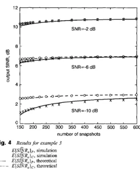
Example 3: Here, we consider the ESB adaptive beam- forming using the 2

D

array and its partitioning shown by Fig. 2a. The desired signal and two uncorrelated interferers are equipowered and impinging on the array from (u~,v,)=(O,O), (uz,vz)=(0.4,0.6), and (u3,v3)=(0.2,0.7), respectively. Fig. 4 shows the results regarding the expectation of the output SINR against the number of snapshots for the cases of SNR = -2 dB, -6 dB, and

-

10 dB. Each result is the average of 500 independent runs. The curves represent the theoretical results based on the formulas given by eqns. 24 and 25. The symbols represent the simulation results using the proposed and conventional techniques. Again, this figure shows the effectiveness of the proposed technique and confirm the performance analysis presented in Section 4.2.

6 Conclusion

This paper has presented an efficient technique for the computation of signal subspace which is required for array signal processing. We partition the entire array into several nonoverlapped subarrays and compute the signal subspaces spanned by these subarray data vectors. Then, these subspaces are utilised to construct the entire signal subspace. It has been shown that, as compared to existing techniques, the proposed technique provides a significant saving in computational burden. Moreover, the proposed technique possesses the advantages of coping with the situations of source number overestimated and array ambiguity over conventional techniques. Statistical performance for each of bearing estimation and eigenspace-based

(6)

adaptive beamforming using the proposed technique has been evaluated. The theoretical works have been illustrated and confirmed by several simulation examples.

7 Acknowledgments

{ A s } which has rank equal to P and the other one is range { Cs}

n

range {As}’ which has rank equal to M-P. Due to the fact that HCs is a full rank square matrix and the matrix given by:

cs(

cFcs)-’

cF(HT G N ) (27)

This work was supported by the National Science Council

under Grant NSC86-22 13-E002-054. represents a projection of the matrix _{Cql,it follows that the matrix given by eqn. 27 is a full

@GN

onto the range 8 1 2 3 4 5 6 7 8 9 10 1 1 12 13 14 15 16 17 18 9 References

SCHMIDT, R.O.: ‘Multiple emitter location and signal parameter estimation’, IEEE Trans. Antennas Propag., 1986, AP-34, pp. 276-280 ROY, R., and KAILATH, T.: ESPRIT - estimation of signal parameters via rotation invariance techniques’, IEEE Trans. Acoust. Speech Signal Process., 1989, ASSP-37, pp. 9 8 4 9 9 5

CHANG, L., and YEH, C.-C.: ‘Performance of DMI and eigenspace- based beamformers’, IEEE Trans. Antennas Propag., 1992, 40, pp.

13361347

KIM, J.W., and UN, C.K.: ‘A robust adaptive array based on signal subspace approach’, IEEE Trans. Signal Process., 1993, 41, pp. 3166-

3171

FELDMAN, D.D., and GRIFFITHS, L.J.: ‘A projection approach for robust adaptive beam-forming’, IEEE Trans. Signal Process., 1994,42, YANG, J.-F., and LIN, H.-T.: ‘Adaptive high-resolution algorithms for tracking nonstationary sources without the estimation of source number’, IEEE Trans. Signal Process., 1994, 42, pp. 563-571

MATHEW, G., REDDY, VU., and DASGUPTA, S.: ‘Adaptive estimation of eigensubspace’, IEEE Trans. Signal Process., 1995,43, pp. 401-

41 1

XU, G., ZHA, H., GOLUB, G., and KAILATH, T.: ‘Fast algorithms for updating signal subspaces’, IEEE Trans. Signal Process., 1994, 41, pp.

537-548

CHAMPAGNE, B.: ‘Adaptive eigendecomposition of data covariance matrices based on first-order perturbations’, IEEE Trans. Signal Process., 1994, 42, pp. 2758-2770

YANG, B.: ‘Projection approximation subspace tracking’, IEEE Trans. Signal Process., 1995, 43, pp. 95-107

RABIDEAU, D.J.: ‘Fast, rank adaptive subspace tracking and applica- tions’, IEEE Trans. Signal Process., 1996, 44, pp. 2229-2244 ERIKSSON, A., STOICA, P., and SODERSTROM, T.: ‘On-line subspace algorithms for tracking moving sources’, IEEE Trans. Signal Process., 1994,42, pp. 2319-2330

MARCOS, S., MARSAL, A., and BENIDIR, M.: ‘The propagator method for source bearing estimation’, Signal Process., 1995, 42, pp.

121-138

pp. 867-876

WAX, M., and KAILATH, T.: ‘Detection of signals by information theoretic criteria’, IEEE Trans. Acoust. Speech Signal Process., 1985,

ASSP-33, pp. 387-392

GOLUB, G.H., and VAN LOAN, C.F.: ‘Matrix computations’ (The

Johns Hopkins University Press, Baltimore, MD, 1983)

LI, E, and VACCARO, R.J.: ‘United analysis for DOA estimation algorithms in array signal processing’, Signal Process., 1991, 25, pp.

147-1 69

-

. ,

_-_

KAVEH, M., and BARABELL, A.J.: ‘The statistical performance of the MUSIC and minimum-norm algorithms in resolving plane waves in noise’, IEEE Trans. Acoust. Speech Signal Process., 1986, ASSP-34, pp.

331-341

YEH, C.-C., LEE, J.-H., and CHEN, Y.-M.: ‘Estimating two-dimen- sional angles of arrival in coherent source environment’, IEEE Trans. Acoust. Speech Signal Process., 1989, ASSP-37, pp. 153-155

Appendix

9.1 Proof of Theorem 1 Here, we prove Theorem 1.

Theorem I : Let

6s

be a basis matrix that spans range {As}, then the matrix given by:

G, = Cs(HC,)-’Gs, (26)

spans range {A,}

Prooj Let GN be an ~x (M-P) full rank matrix which sati_sfies ,4$GN = 0 or A$ (HTGN) 0. Therefore, the rank of GN is M-P and the rank of HHGN is also M-P because H is row selecting _matrix which selects the linearly independent rows of GN. Since range { A s }

c

razge {C,} and we note from eqn. 7 that Cs is of size M x M and full rank with rank equal to M , range {Cs} can thus be decomposed into two orthogonal subspaces. One is range

240

rank ‘matrix with rank equal t o M-P- and spans range

CCs}-n

range {As}’. Moreover, by using the fact that G: GN= 0 and HCs is a full rank square matrix, it is easy to show that Gs given by eqn. 10 is a full rank matrix which is contained in range {Cs} and orthogonal to the matrix given by eqn. 27. As a result, we have range { Gs} =range

{ A S } .

0

9.2 Proof of theorem 2 Here, we prove theorem 2.

Theorem 2: Assume that the Gsk given by eqn. 6 are full rank basis matrices such that range {ASk}_E range (GSk} for k = 1, 2,. . . , K. Then y e have (a) If

Gs

is a full rank matrix such that range { A s } =range { G s } , then range { A s } =range_ { Gs}. (b) If

9,

is a full rank matrix such that range { A s }

c

range

{Gs},

then range { A s }

c

range Pro08 From the assumptions that range {Ask} 2 range {Gsk}, we note that range { A s }

c

range { C s } since C N

given by eqn. 7 is still orthogonal to As. Moreover, it can be shown that the matrix of eqn. 27 is contaited in range {$} and orthogonal to range { A s } if range ( A s }

C

range { G s } . As a result, the matrix Gs given by eqn.; 0 is always a full rank matrix with rank equal to that of Gs and range { A s } range (Gs}

c

range { C s } . Therefore, we have the result of (a) if Gs bas rank equal to P. In contrast, we have

0 c

GS}.

the result of (b) if Gs has rank greater than I?

9.3 Mean squared estimation error

Here, the mean squared estimation error using the proposed technique for bearing estimation is derived. From eqn. 10, we construct an NS basis matrix which satisfies G# Gs= 0 as follows:

GN = [ J ~ E N ~ , J ; E N ~ ,

.

. . , JGENK, H T E ~ ] (28) Accordingly, the corresponding NS basis matrix of using finite samples can be written as

wherenkNk qpd

gN

represent the basis matrices associated with R and

k,

respectively. Thus, the search function under finite samples becomes

$4)

zz A ( + ) H G N ( G ~ G N ) - ’ G ~ A ( 4 ) (30)

Let the ith direction angle estimated be

qL.

Using the first- order approximation presented by [16], it can be shown that the resulting estimation error is approximately given by

A+, - ( B ( ~ , > H G “ . i ( 4 , > > - 1 R e { B ( + ~ ) ~ ~ G ~ A ( + , ) } (31)

where Re{x} denotes the real part of x. A

(4,)

is the first- order derivative of A ( + ) at

+

=

+,,

SGN= GN-GN and

(32)

1 H ’

B(4,)

= ( G C G N ) -

(7)

From eqn. 3 1, we can show that the mean squared estimation error is approximately given by

where

F, =

(k:&)-',

Bk(f$r) contains the entries of

~ ( 4 , )

from the

(Cfzi

(M,--P,)

+

1)th entry to the ( (M,-P,))th entry, and B(4,) contains the last M-P entries of B ( 4 J . up, denotes the ith column of the identity matrix Ip. Finally, substitut- ing eqn. 39 into eqn. 33 yields the result shown by eqn. 18. IEE Proc -Radar, Sonar Navig , Vol 146, No 5. October 1999

9.4 Output SlNR

Under finite data samples, the computed SS basis matrix Gs can be expressed as

Gs = G,

+

SG, (41)

where SGs approaches zero as the number of data snap- shots increases. We decompose 6Gs into two components which are in the signal and noise subspaces, respectively, as follows

JG, = G,(G:G,)-~G;sG,

+

G~(G,HG,)-'G;sG, (42) Substituting eqn. 42 into eqn. 41 yields

-1 H

G,

= G ,

+

SG, = (G,

+

AG,)(I~

+

( G ~ G , ) G, SG,) (43) where AG, =

(z,

- G,(G;GJ~G:) x SG,(I,

+

( G ; G , ) - ~ G ~ s G , ) - ' (44) We note from eqn. 43 that I p + , ( G f G s ) - ' G ~ S G s is full rank and hence invertible if SG, is small enough and then the term (GfG,)-'G~SG, can be neglected as compared to Ip. Thus, these two matrices Gs+AGs and Gs span the same subspace. As a result, ESB adaptive beamforming based on these two matrices will produce the same optimal weight vector. It follows that

AG, E range{GN}, AG:RG, = 0, and

G:46,,

4,)

= Gf&B,,

4,),

(45) for i = 1, 2 , . . . , P Moreover, we have the following two approximations from eqn. 23:

G ~ R G , E

r,

+

AG:RAG, ₍₄₆₎

and

Fs

=

r,

+

A r , 2:

r,

+

AG;RAG, (47) Computing the inverse of eqn. 47 and utilising the general- ised matrix inversion lemma under the assumption of

ATs

<<

rs,

we obtain the following approximation:

x - ril A T s s r-l (48)

Substituting eqn. 47 into eqn. 23 and taking the difference of eqn. 23 and eqn. 22, we obtain

AWo = WO - WO % AG,Ti1G,HA(61,

41)

- G , I ' ~ l A T ' S I ' ~ l G ~ A ( O 1 ,

41)

(49)

Based on eqn. 49, we obtain the output power of the desired signal and the total array output power as follows:

I;, = 711 lA(4,

4JHG0l2

% p ,

+

Apsl

+

the first and higher-order terms

it

= GfRG, %pt

+

Aptl

+

Apt2

+

the first and higher-order terms (50)

(8)

respectively, wherep, andp, denote the output power of the desired signal and the total array output power without finite sample effect and are given by

Ps = nllA(eI7 41FWol2 = nl('Wl9 4 1 ) H G s G ' G ? A ( h

41N2

pt = WFRW, =A(B1, 41)HGsTi'GfA(B1, 41) (51) respectively, and Apsl = q ( A ( e 1 , 4 1 ) H G s ~ , ' A ~ s r i 1 G ? A ( e l ,

4 1 ) ) ~

Aptl = A(81, 4 1 ) H G s ~ ~ 1 A ~ s ~ ~ 1 A ~ s r ~ 1 G ? A ( e l ,

41)

Apt2 = nn,A(81, 4 1 ) H G s ~ , 1 A G f A G s r i ' G ~ ~ ( e l , 41) (52) represent the corresponding second-order terms, respectively. Following eqn. 52 and the property of eqn. 51, we can easily show that

1 P

EIAPsl} = ,P,, and E{APtl} = ,Pt (53)

Using the above results and taking the first-order approximation, we can hrther show that the expectation of the array output SINR is approximately given by

E{s%R,} 2: SINR, 1 - L-'(SINR,

+

I)(P - 1).

- L - ' ~

(

E(LApt2} Pt -Ps

1

P 4 ) This approximation is possible because the expectations of all first-order terms are zero and higher-order terms are negligible as compared to the second-order terms, where SINR, =ps/(p,-ps) denotes the array output SINR without the finite sample effect.

Similarly, the basis matrix for the noise subspace obtained from finite snapshots can be expressed as

GN

= GN

+

6GN (55)

Hence, we have

GcGs = (GN

+

c~G,)~(G,

+

6Gs) = 0 (56) It follows from eqn. 56 that

GC~G,

2 -~G;G, (57)

by neglecting the second-order terms in eqn. 56. Substitut- ing eqn. 57 into eqn. 44 and neglecting the higher-order terms yields

AGs 2: -GN(GEGN)-16GcGs (58)

E{ LApt2} = n, Tr{ (G; GN)-l @)

@ = E{LGG; W, W~SG,}

Based on eqn. 22, eqn. 52, and eqn. 58, we can obtain (59)

(60) where

Let @hk for h, k = 1,2,

. . .

, K be the submatrices containing

the rows from the (C:={ (Mi-Pi)+ 1)th row to the (Cf=l

(Mi-Pi))th row and the columns from the (C:=\

(Mi-Pi)

+

1)th column to the (C;=, (Mi-Pi))th column of @, @ h ( K c 1 ) for h = 1, 2 , .

. .

, K be the submatrices taking the rows from the (C?=', (Mi-Pi)+ 1)th row to the (Mi-Pi))th row and the last I@-P columns Of @, and

@ ( K + l ) ( K + l ) be the submatrix taking the last M-P rows

and columns of @. Using eqns. 37 and 38, we can show

From eqn. 62, we observe that & k = O because Jh and Jk select two nonoverlapped subarrays if h

#

k. Since

nnR&

= E s k F& n, pglFsk E$, we can easily show that all of Qkk, 9,+ 1) and 9(,+ ' ) ( K c 1 ) decreases as the input

SNR increases.

Finally, consider the term p,-p? which represents the array output interference plus noise power and can be written as pt-ps =

e

(RI+ n,Z,>

W,,

where RI denotes the correlation matrix due to the interference only. Based on eqn. 59, we can rewrite the third term in the right-hand side of eqn. 54 as follows:

Eqn. 67 decreases as the input SNR increases since its numerator decreases, while its denominator increases as the input SNR increases. In contrast, the second term of

eqn. increases as the input SNR increases. Therefore, the third term of eqn. 54 becomes negligible as compared to the second term of eqn. 54 as the input SNR increases. That is, eqn. 54 is approximately given by

E(SI^NR,} 2: SINRo(l - L-'(SINRo

+

1)(P - 1)) (68) when the input SNR is high enough.

Efficient Computation of the Eigensubspace for Array Signal Processing