利用主成份分析監控剖面資料之研究

(1)

國

立

交

通

大

學

統計學研究所

碩

士

論

文

利用主成份分析監控剖面資料之研究

Profile Monitoring via Principal Components

研究生：王筱娟

指導教授：洪志真博士

(2)

利用主成份分析監控剖面資料之研究

Profile Monitoring via Principal Component

研究生：王筱娟 Student：Hshiao-Chuan Wang

指導教授：洪志真 Advisor：Jyh-Jen Horng Shiau

國立交通大學

統計學研究所

碩士論文

A Thesis

Submitted to Institute of Statistics National Chiao Tung University in Partial Fulfillment of the Requirements

for the Degree of Master

in Statistics June 2008

Hsinchu, Taiwan, Republic of China

(3)

誌

謝

兩年的碩士班生涯即將結束，馬上就要走入人生另一個旅程，

回首剛回到校園進修時的期待，以及現在收成的喜悅，這一切都要感謝許多人對我的提攜與幫助。這一篇論文能夠順利完成，首先要感謝我的指導老師－洪志真教授。感謝老師給予我細心的指導與叮嚀，並在數次的修改中，給予我細部的指導，論文方能夠如期的完成。除此之外，有感謝我的口試委員陳鄰安教授、黃榮臣教授及曾勝滄教授，在百忙之中為我口試，在口試時對於我的指導，更讓我發現本論文主題可以更深入探討的地方，這在我的工作領域上有很大的幫助，能夠真正達到學以致用的目標。而我的同學們在這段時間給予了很多的協助，尤其是在我工作繁忙時，幫我解決了很多事務上的問題，讓我可以專注在論文的題目上。我要特別感謝怡玲和香菱，在課業及論文的撰寫給予我寶貴的建議及鼓勵。也感謝統計所上的同學，在碩二繁忙的日子裡帶給歡樂，減輕寫論文時的壓力。除此要特別感謝我們所上的助理郭碧芬小姐，她不辭勞苦幫我們處理很多行政事務上的問題。最後要感謝我的家人給予我莫大的支持，與家人相處的時間很少，因為爸媽的體諒，才能專心完成學業。另外還有很多曾經幫助過我的朋友，因為有大家的幫助，我才能有今天的成果。

(4)

利用主成份分析監控剖面資料之研究

研究生：王筱娟指導教授：洪志真博士

國立交通大學統計學研究所

摘要

在多數的品質監控應用上，我們使用一個或多個品質特性 (一個變數或多個變數) 來測量製程的品質。然而，在許多情況下，有興趣的反應變數不是一個變數，而是一個函數。這個函數稱為剖面 (profile)。本研究中我們採用無母數的模型去監控剖面資料而不是用有母數的模型。對於剖面資料間可允許的變化，我們利用主成份分析分析剖面資料變異的結構。我們利用剖面資料所包含的主成份分數(Score)的資訊監控剖面資料。傳統的統計量視每一個主成份同等重要。然而，對於貢獻解釋剖面的變異較少的主成份而言，當他們的分數與製程在控制中的值有顯著不同時，在實務上我們未必希望因此而發出失控警訊。換句話說，這些主成份的影響在統計上是顯著的，而在實際上卻並不重要。因此我們提出一個新的監控方法，其只對於重要的主成份改變時是敏感的。我們用模擬來檢驗此方法的效能。 2 T i

(5)

Profile Monitoring via Principal Components

Student: Hshiao-Chuan Wang

Advisor: Jyh-Jen Horng Shiau

Institute of Statistics

National Chiao Tung University

Hsinchu, Taiwan

Abstract

In most of quality control applications, we use one or multiple quality character-istics (a single univariate or multivariate variable) to measure the process quality. However, in many situations, the response of interest is not a single variable but a function of one or more explanatory variables. This functional response is called a profile. We adopt nonparametric models to monitor profiles rather than parametric models.

For profiles with allowable profile-to-profile variation, we utilize the technique of principal components analysis to analyze the covariance structure in profiles. We consider monitoring profile by using the information contained in the principal component scores. Classical T2 statistics treat each principal component equally important. However, for some principal components with little contribution in ex-plaining the variability of profiles, it may not be desirable to signal out-of-control alarms when their scores are significantly different from the in-control values. In other words, effects of these components are statistically significant but not practi-cally significant. Thus, we propose a new monitoring scheme that is only sensitive to shifts on “important” components. Simulation studies demonstrate the efficacy of the method.

(6)

List of Tables

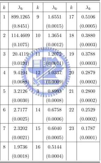
1 Eigenvalues for smoothed VDP data (proportion of explaining variation) . 20

2 ARL for PC1 . . . 21 3 ARL for PC2 . . . 21 4 ARL for PC23 . . . 22 5 ARL for PC1( m=200) . . . 22 6 ARL for PC2( m=200) . . . 23 7 ARL for PC23( m=200) . . . 23 8 ARL for PC1( m=300) . . . 24 9 ARL for PC2( m=300) . . . 24 10 ARL for PC23( m=300) . . . 25 11 ARL for PC1( m=400) . . . 25 12 ARL for PC2( m=400) . . . 26 13 ARL for PC23( m=400) . . . 26 14 ARL for PC1( m=500) . . . 27 15 ARL for PC2( m=500) . . . 27

(9)

16 ARL for PC23( m=500) . . . 28

17 ARL for PC1( m=600) . . . 28

18 ARL for PC2( m=600) . . . 29

(10)

List of Figures

1 Original 24 VDP-profiles . . . 30 2 Smoothed VDP . . . 30 3 Density for T3 . . . 31 4 Power of PC1 (true VDP) . . . 32 5 Power of PC2 (true VDP) . . . 32 6 Power of PC23 (true VDP) . . . 32

7 Power for PC1 with m=200 . . . 33

(11)

(12)

1 Introduction

Statistical Process control (SPC) has been widely applied in many areas, especially in industries. Classical methods for SPC usually assume that the quality of the product or process can be measured by one or multiple quality characteristics. However, in many situations, the response of interest is not a single (univariate or multivariate) quality variable but a function of one or more explanatory variables. For example, for a product item, we collect a set of measurements over time, space, or levels of parameter settings in production or experiments, etc. This functional response data is called a profile. An example of profiles given in Kang and Albin (2000) is the dissolving process of aspartame, an artificial sweetener, which is characterized by the amount of aspantane dissolved per liter of water at different levels of temperature. Mestek et al. (1994) used linear functions to monitor the performance of the process for the calibration of a mass flow controller. An interesting example of nonlinear profiles was presented in Walker and Wright (2002). The density of a particle board is measured with a profilometer that uses a laser devices to take measurements at fixed depths across the thickness of the board. These measurements on the sample form the vertical density profile (VDP) of the board. The VDP dataset contains 24 profiles of vertical density and each profile consists of 314 measurements taken 0.002 inches apart. The original 24 VDP profiles are shown in Figure 1. As to some other work in profile monitoring, Woodall, Williams, and Birch (2004) provided a good introduction to profile monitoring and its applications. For other related works, see in Jensen et al. (2007), Williams et al. (2007), and the reference cited therein.

Shiau and Weng (2004) extended the linear profile monitoring schemes of Kang and Albin (2000) and Kim et al. (2003) to profiles of more general forms. Fixed effects models are considered in these papers. Kang and Albin (2000) monitored linear profiles with a fixed effects model by monitoring slopes and intercept jointly with a multivariate T2

charts. However, under the fixed effects model, the effects of some uncontrollable factors, such as variations in humidity or temperature, are all categorized as part of the error term. In many cases, the collective effects of these factors may affect the values of the

(13)

slope and intercept of the linear profiles. If so, then these hard-to-control factors would be more appropriate to be considered as common causes of variation. Shiau, Lin, and Chen (2006) proposed an approach to monitoring linear profiles with a random effects model to account for these common causes of variation. In this study, we consider a parametric random effects model in order to incorporate more variability that we often observe in many profile data. To understand the profile-to-profile variation, we focus on the covariance structure of profiles. To analyze the covariance structure, we consider the technique of principal components analysis (PCA).

Classical Hotelling T2 statistic treats all the principal components equally important. However, for principal components with little contribution in explaining the variability of the profiles, it may not be desirable to signal alarms when the corresponding scores are significantly deviated from the in-control process. This is an example of effects being sta-tistically significant but not practically significant. We propose a new monitoring scheme that is only sensitive to shifts in “important” components. This method gives a weight to each principal component according to how much of the total variation it accounts for. By putting more weights on “important” components, we can detect shifts in these corre-sponding directions more effectively. Also by neglecting those principal components that contribute so little to the total variation, we can avoid unnecessary interrupts signaled by the shiftings in the corresponding directions.

We apply the principal components analysis to data to obtain the eigenvectors and the associated principal component scores. When the covariance matrix is not of full rank, some eigenvalues are zero. When this happens, neglect the eigenvectors associated with them. This will happen when the number of profiles is smaller than the number of the set points. This problem also can be solved by using the singular value decomposi-tion (SVD) to data matrix. See Ramsary and Silvermen (2005). Then we utilize these eigenvalues/eigenvectors to construct monitoring statistics for Phase II profile monitoring.

(14)

statistic, and a total-squared-scores T2 statistic. A simulation study is conducted to evaluate the performances of the three statistics. It is found from the simulation study that the total-squared-scores T2 statistic has better power than the classical Hotellong T2 statistic and maximum score statistic for shifts in the most important principal component and is very insensitive to the “unimportant” principal components.

The rest of the thesis is organized as follows. Section 2 reviews the technique of PCA, which is employed to analyze the covariance structure of the in-control profiles, and the concept of functional data analysis. Section 3 describes the three monitoring schemes studied in this paper. Section 4 presents the simulation results of Phase II profile monitoring with the VDP example. Finally, Section 5 concludes the paper with a brief summary and some remarks.

2 Review on Background Methodologies

In an increasing number of cases, the quality of a product or a process cannot be rep-resented by a single quality variable. Rather, a set of measurements are taken across some continuum, such as time or space. In this section, we review the concepts of profile monitoring, nonparametric regression, principal components analysis, and functional data analysis.

2.1 Nonparametric Regression

Using linear models to monitor nonlinear profiles definitely is not suitable. By treating the discretized profile as a vector, monitoring nonlinear profiles can be considered as a par-ticular application of multivariate process control problems. However, many traditional statistical methods fail when dealt with functional data, e.g., the strong correlations

(15)

be-tween the variables will cause an ill-conditioned problem in multivariate models. Hence, nonparametric statistics have been developed accordingly. Recently, more and more re-search works have focused on monitoring nonlinear profiles. A common approach to non-linear profile monitoring is to fit a parametric regression model to each profile and make inferences based on the estimated parameters. When a parametric form of the profiles is overly complicated or hard to determine from data, the nonparametric regression approach may be more appropriate. This approach fits profiles via some smoothing methods, like spline smoothing, local polynomial smoothing, and wavelets. The following nonparametric regression model is considered:

y_j = m(xj) + εj, j = 1, ..., p, (1)

where yj is the j-th observation of the profile, m(x) is a smooth regression curve to be

estimated and εi are independent and identically distributed (i.i.d.) normal variates with

mean zero and common variance. Each profile in the VDP data set is smoothed by the function “smooth” of statistical package R. Figure 2 shows the 24 smoothed VDP profiles.

2.2 Functional Data Analysis

There is an increasing number of situations coming from different fields of applied sciences in which the collected data are curves. However, the progress of the computing tools, both in terms of memory and computational capacities, allows us to deal with large sets of data. And we can observe a very large set of variables. In some situation, the variable can be observed over a period of time T = [T0, T ], then the observation can be expressed as a

family of random variables, denoted by {X(t), t ∈ T }. Since the functional data consist of noises that may affect the performance of analysis, smoothing techniques can filter out the noise and then the features revealed by PCA can explain the data more clearly.

(16)

function Q(s, t) as below: ¯ X(t) = n−1 n X i=1 Xi(t), (2) Q(s, t) = (n − 1)−1 n X i=1 {Xi(s) − ¯X(s)}{Xi(t) − ¯X(t)}. (3)

Then, we can use the principal components analysis for the functional data to analyze the profile.

2.3 Principal Components Analysis

The principal components analysis (PCA) is very useful in summarizing and interpreting profiles with the same equally-spaced values for independent variable. The PCA is a tech-nique for choosing more important combinations of these independent variables. Castro et al. (1986) showed that the principal modes of variation contain eigenfunctions of the process covariance function. The authors also gave methods for estimating these eigenfunc-tions from a set of observed curves. Rice and Silverman (1991) provided a nonparametric method to estimate the mean function from a set of curves under the assumption that it was smooth. They also suggested a variant of the usual cross-validation to choose the degree of smoothing for data to be smoothed. In the estimation of the covariance struc-ture, they primarily concerned about the first few eigenfunctions that were smoothed and their eigenvalues decayed rapidly. Jones and Rice (2002) suggested to use a simple PCA to identify important modes of variation among these curves. And they also used the principal component scores to identify particular curves that demonstrate the form and extent of a particular mode of variation.

Below, we review the PCA with materials mainly taken from Anderson (2003). The PCA is a multivariate procedure that rotates the data set such that the maximum vari-abilities are projected onto the new axes. Essentially, a set of correlated variables are transformed into a set of uncorrelated variables. Then, these uncorrelated variables are called principal components (PC). These principal components are linear combinations of

(17)

the original variables. And the main concept is to reduce the dimension of the data set while retaining as much information as possible. Principal components contain special properties or features of the covariance matrix. They turn out to be the eigenvectors of the covariance matrix. Let the random vector Y of p components have the covariance matrix Σ and assume that the mean vector of the random variable Y is zero without loss of generality.

Theorem 1 (Anderson, 2003)

Let Y be a p-component random vector with E(Y) = 0 and E(YY0) = Σ. Then there exists an orthogonal transformation B such that

U = B0Y (4)

has the covariance matrix

Λ =               λ1 0 0 . . . 0 0 0 λ2 0 . . . 0 0 0 0 λ3 . . . 0 0 .. . ... . .. ... ... ... 0 0 . . . 0 λp−1 0 0 0 . . . 0 0 λp               , (5)

where λ1 ≥ λ2 ≥ . . . ≥ λp ≥ 0 are roots of |Σ − λI| = 0. And the r-th column of

B, βr, satisfies (Σ − λrI)βr= 0. And the r-th component of U, Ur= β0rY has maximum

variance of all normalized linear combinations uncorrelated with U1, . . . , Ur−1.

Thus, β1, . . . , βp are eigenvectors and λ1, . . . , λp are eigenvalues of the covariance

ma-trix Σ. In PCA, βr is the r-th principal component of Y and Ur is called the score of the

r-th principal component. These scores will catch the features of curves in the directions of the corresponding principal components. In our monitoring scheme, we aim at detecting changes based on these principal component scores.

(18)

When analyzing data, we apply PCA to the sample covariance matrix S. Suppose we have n profiles and each profile contains p measurements. Compute the sample covariance matrix S by S = 1 n − 1 n X i=1 (y_i− ¯y)(y_i− ¯y)0, (6) where y_i the i-th profile and ¯y is the mean vector of these profiles, and ¯y = Pn

i=1yi/n.

Apply the eigenanalysis to the sample covariance S. The eigenvector corresponding to the j-th largest eigenvalue is the j-th principal component, j = 1, . . . , p. Then project each profile onto the eigenvectors to get the PC scores.

2.4 Functional PCA vs. PCA

In this study, we consider the nonparametric model of Karhunen-Lo`eve expansion to model profile data. Let {X(t), t ∈ T } be a realization of a stochastic process with mean µ(t) and covariance function G(s, t), where

Cov(X(s), X(t)) = G(s, t) =

∞

X

k=1

ρkφk(s)φk(t)

and {φ1(t), φ2(t), . . .} is an orthognormal sequence of continuous eigenfunctions in L2 and

eigenvalues ρ1 ≥ ρ2 ≥ . . . ≥ 0 satisfy

Z

T

G(s, t)φk(t)dt = ρkφk(s), k = 1, 2, . . . (7)

Equation (8) is the functional eigenequation. Then X(t), t ∈ T , has a (quadratic mean) representation: X(t) = µ(t) + ∞ X k=1 Xkφk(t), (8)

where Xk=R (X(t) − µ(t))φk(t)dt. It is well known that Xkfollows a normal distribution

with mean zero and variance ρk and {Xk} are linearly independent. In equation (9), the

common modes of variation of a curve are represented by the Karhunen-Lo`eve expansion in L2.

(19)

In practice, we observe the curve data at some discrete points as in the following: Yj = X(tj) + εj, j = 1, . . . , p. (9)

We apply Tukey’s smooth smoothing techique code as a function in R to filter out the noise. After filtering out the noise εj, the actual signals of curves can be better extracted

from the data and these signals can explain the variation of profiles more clearly.

In this study, we adopt the functional data analysis approach to model profiles data but computation is carried out for discretized profiles. Therefore, we need to understand the relationship between the eigenfunctions and eigenvectors.

Let Y1, . . . , Ymbe m discrete profiles data measured at the same p equally-spaced points

t1, . . . , tp. The standard multivariate principal components analysis produces eigenvalues

λ and eigenvectors u satisfying

V u = λu, (10) where V is the sample covariance matrix of Y1, . . . , Ym. Note that the sample covariance

matrix V has the elements V (tj, tk) where V (·, ·) is the sample covariance function. Let ξ

be any function and ξ = (ξ(t1), . . . , ξ(tp))0. Let w = |T |/n, where |T | is the length of the

interval T . Since Z V (tj, t)ξ(t)dt ≈ w p X k=1 V (tj, tk)ξ(tk),

the eigenfunction (8) can be approximated by

wV ξ = ρξ. (11) The solution of (12) will correspond to those of the ordinary discrete eigenequation

V u = λu with ρ = wλ and ξ = w−1/2u if wkξk = kuk = 1.

(20)

k-th eigenvalues and eigenvectors of the sample covariance matrix. Let Xk and Ak be the

scores of the functional PCA and PCA respectively. Then the score in functional PCA Xk =R (X(t) − µ(t))φk(t)dt ≈ wPp_j=1(X(tj) − ¯X(tj))φk(tj)

= wPp

j=1(X(tj) − ¯X(tj))w−1/2βkj = w1/2Ak

Accordingly, we have X_k2/ρ2_{k k}/λk and Pp_k=1Xkφk ≈Pp_k=1Akβk. This means that we can

approximate the functional PCA by multivariate PCA.

3 Monitoring Schemes

3.1 Monitoring Statistics

In this study, we focus on Phase II monitoring. In Phase II study, it is usually assumed that the in-control process is already characterized. Then, without loss of generality, as-sume the discrete in-control profiles are i.i.d. as Np(0, Σ) and Σ is known. It is well

known that, when the process is in control, the score Ak is distributed as N (0, λk). For

example, see Anderson (2003). Consider the case of shifts in mean. Let δ be the shift size as a multiple of standard deviation. In this thesis, for Phase II monitoring, we study three types of control charts based on the PC scores as described below. Denote the number of nonzero eigenvalues by n0. The first chart is the usual T2chart, the the monitoring statistic:

T1 = n0 X k=1 λ−1_k A2_k. (12) Since Ak is distributed as N (0, λk), Ak/ √

λk follows the standard normal distribution.

Then T1 is distributed as χ2 with n0 degrees of freedom. Thus, claim the process as out

of control if

(21)

where χ2_1−α,n0 denotes the 100(1 − α) percentile of the χ2 distribution with n0 degrees of freedom. By (13), it is clear that T1 statistic treats each principal component (score)

equally important.

Note that PC scores can be monitored individually since they are independent. But it would be too troublesome to monitor several charts at the same time. Thus we consider a combined chart scheme that combines all n0 individual PC score charts. More specif-ically, a combined chart signals when any of the individual charts signals. This scheme is equivalent to monitor the maximum of the individual monitoring statistics. Then the monitoring statistic is as below:

T2 = max

1≤k≤n0|λ

−1/2

k Ak|. (14)

Thus, signal is out of control if

T2 > Zα0_/2, (15) where α0 = 1 − (1 − α)1/n0_{. Then it can be easily shown that the false alarm rate ofthe}

combined chart is α.

The first two approaches are often used in other contexts. The third approach is new and proposed practially for profile monitoring. The idea is simple. We wish to find a mon-itoring statistic that are sensitive to the shifts in “important” directions and insensitive to the shifts in “unimportant” directions. For simplicity, consider the following monitoring statistics: T3 = n0 X k=1 A2_k. (16) Note that T3treats each of principal components differently with a weight according to how

(22)

component score to standard normal. Satterwaite (1941) proposed an approximation to linear combinations of independent χ2

1distributions as a scaled χ2 distribution, cχ2df, where

c = Pn0 k=1λ 2 k Pn0 k=1λk and df = [ Pn0 k=1λk] 2 Pn0 k=1λ 2 k . (17)

Thus, the process is claimed out of control if

T3 > cχ2df,1−α. (18)

To see whether the control limit given in (19) is adequate or not, as an example, we generate 1,000,000 profiles from the eigenvectors/eigenvalues of the smoothed VDP data to approximate the distribution of T3. The density of T3 estimated by kernel density

estimation is shown in Figure 3. Since the approximate distribution of T3 is not close

enough to cχ2

df, we proposed using empirical (1 − α)th quantitle of T3 as the control limit

of this chart. We refer to this chart as the “Total-Squared-Scores” chart hereafter.

3.2 Control Limits

In studying the performances of the monitoring schemes, researchers usually assume µ and Σ are known in Phase II monitoring. In this study, we evaluate the performances of the proposed monitoring schemes in terms of the average run length (ARL). Several versions of control limits are considered as below.

1. T2 _Chart:

For T2 _{statistic, we consider another version and refer to the original T}

1 statistic in (12) as T11 = n0 X k=1 λ−1_k A2_k. (19) Since T11 has poor power when n0 is large, we consider a T2 statistic by adding only

the tanderized scores of effective components as T12 =

K

X

k=1

(23)

where K is the number of the “effective” principal components. It is obvious that T11

and T12 have chi-squre distributions with degrees of freedom n0 and K, respectively.

Then the control limits for T11 and T12 are χ2n0_,1−α and χ2_K,1−α, respectively.

2. Combined Chart:

The control limit of T2 is Zα0_/2, where α0 = 1 − (1 − α)1/n 0

.

3. Total Squared Score (TSS) Chart:

Since Figure 3 shows that the distribution of T3 is not close to cχ2df, we study two

versions of control limits: one is the empirical (1 − α) quantitle and the other is

cχ2_df,1−α. For the empirical quantitle, we take the eigenvalues {λk}n

0

k=1 of the smooth

VDP data as the true eigenvalues/eigenvectors and generate 1,000,000 set of {Ak}n

0

k=1

with Ak ∼ N (0, λk), to obtain 1,000,000 T3, and hence the empirical (1−α) quantitle

of T3. We refer to the T2 control chart with this control limit as the T31 chart in

simulation studies. For our simulation study, U CL31 is 8262.107. We refer to T2

chart with the control limit cχ2

df,1−α as the “T32”, where c and df are estimated by

eigenvalues and eigenvectors of the smoothed VDP.

On the other hand, if the parameters are unknown, we need to use some in-control historical data to estimate these parameters. Jensen et al. (2006b) mentioned that the effect of parameter estimation on control chart properties should not be ignored. Thus we consider the case that eigenvalues/eigenvectors are estimated from in-control profiles to investigate the effect of the estimation error. For this cases, the control limits are obtained as below. The T2 _{and the Combined Chart have exact control limits as given above. Fore}

versions of control limits for T3 are considered. The control limit for T31 and T32 are as

the same as above. Assume that we have m in-control profiles available. Apply PCA to them to obtain eigenvalues and eigenvectors, generate 1,000,000 set of scores as before with these estimated eigenvalues to obtain 1,000,000 T₃0s. Let the control limit be the

(24)

Since these estimated parameters depends on this particular set of m profiles, the performance of the control chart may not be the average case. Thus we will repeat the study, say b times to coverage sampling bias. The last version of the TSS Chart is referred to as “T34” chart, in which the control limit is cχ2df,1−α with c and f as in (17) but using

the setimated eigenvalues for {λk}n

0

k=1.

4 Simulation Studies

4.1 Data Generation

In our simulation studies, we simulate data based on the vertical board density profiles. The vertical board density profiles from Walker and Wright (2002) consist of 24 profiles of vertical density, each profile has 314 measurements. These data set is available at http://bus.utk.edu/stat/walker/VDP/Allstack.TXT. First, we smooth each profile and then apply SVD to the sample covariance matrix of VDP data to get the “original” eigenvalues and eigenvectors, {(λk, βk)}, and treat them as the population version. Note

that monitoring the functional data can be reduced to monitoring the discrete profile data as shown in Section 2.4. Thus, we only need to generate discrete profile data. Table 1 gives 23 eigenvalues of the smoothed VDP data. To generate a new profile as a data vector, we use: Y = µ + 23 X k=1 Akβk, (21)

where Ak ∼ N (0, λk), µ is the mean vector of the smoothed VDP data and is assumed

known. Akis the k-th PC score of a profile. When the process is in control, the score Ak is

distributed as N (0, λk). For an out-of-control process, we let the score Ak be distributed

as N (δ√λk, λk). In our study, δ ranges from 1 to 12.

In our simulation study, two methods are considered in Phase II monitoring. One uses the “true” eigenvalues and eigenvectors of the smoothed VDP, the other uses the estimated

(25)

eigenvalues and eigenvectors from m profiles. And each of the m profiles in our study is of the form (21).

For simulation study with “true” eigenvalues and eigenvectors of the smoothed VDP data, we only need to generate {Ak}n

0

k=1 1,000,000 times for each shift in PC1, PC2,

and PC23. For simulation study with estimated eigenvalues and eigenvectors, we first generate m profiles by equation (21). Apply PCA to these m profiles to obtain estimated eigenvalues ˆλ1, . . . , ˆλ23 and eigenvectors ˆβ1, . . . , ˆβ23. Generate 1,000,000 profiles of (21).

Since the mean vector µ of the process is known in Phase II monitoring, without loss of generality, we assume µ=0. Project profiles onto these estimated eigenvectors to get their PC scores. We use these principal component scores to evaluate the performances of the three charts constructed with the statistics T1, T2, and T3 in Phase II monitoring

in terms of the detecting powers. Repeat the above procedure 1,000 times to average the detecting power so that the simulation results can represent an average case, not biased by the particular m profiles used for constructing the control limits. In our study, the false alarm rate α is set at 0.0027 and m=200, 300, 400, 500, 600.

4.2 Number of Principal Components

In this paper, we analyze the VDP data set and its eigenvalues are shown in Table 1. This table shows that the first four principal components account for 0.8451, 0.1076, 0.0192, and 0.0088 of the total variation in the profiles, respectively. The total is 0.9807. Thus, for T12 statistic, K is set at 4 for the monitoring scheme.

4.3 Simulation Results

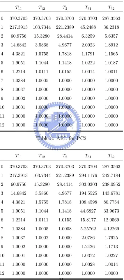
In this studies, the eigenvalues/eigenvectors of the smoothed VDP data are treated as the true population parameters. The performance of the control charts are estimated in terms

(26)

of ARLs. Table 2-4 presents the ARL values of the charts under study on PC1, PC2, and PC23,respectively. Figure 4-6 display the corresponding detecting power of charts. The results are summarized as below:

• Since the T2 _{charts and the combined chart treats each principal component equally}

important, there is no difference in performance among all principal components for them.

• The T2 _{chart using only the effective principal components, T}

12, performs better

than the T2 _{chart using all principal components, T}

11, for all PC scores.

• The combined chart performs in between the two T2 _{charts, but fairly close to the}

T2 chart with only four components for the first four PCs.

• The Satterwaite’s approximation indeed is not good enough for process monitor-ing, which leads to an unsuitable in-control ARL. Hence, this control limit is not suggested.

• The TSS chart using the empirical (1 − α) quantile as the control limit perform better than the T2 charts and the combined chart for PC1.

• The detecting power of the TSS chart drops very quickly after the first component. This confirms the expectation that statistic T3 is insensitive to “unimportant” PCs.

But, the problem is that the TSS chart has very little detecting power for changes in other principal components.

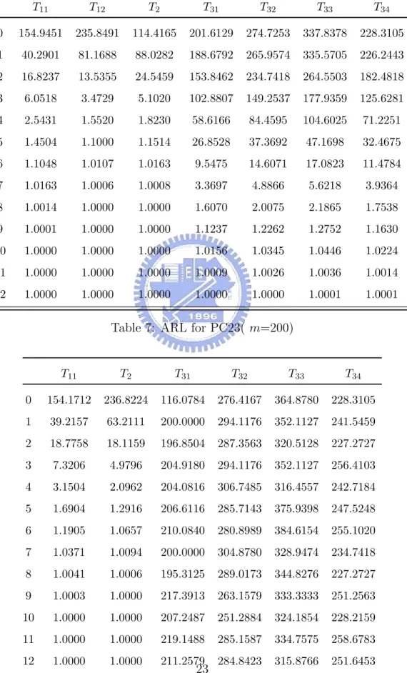
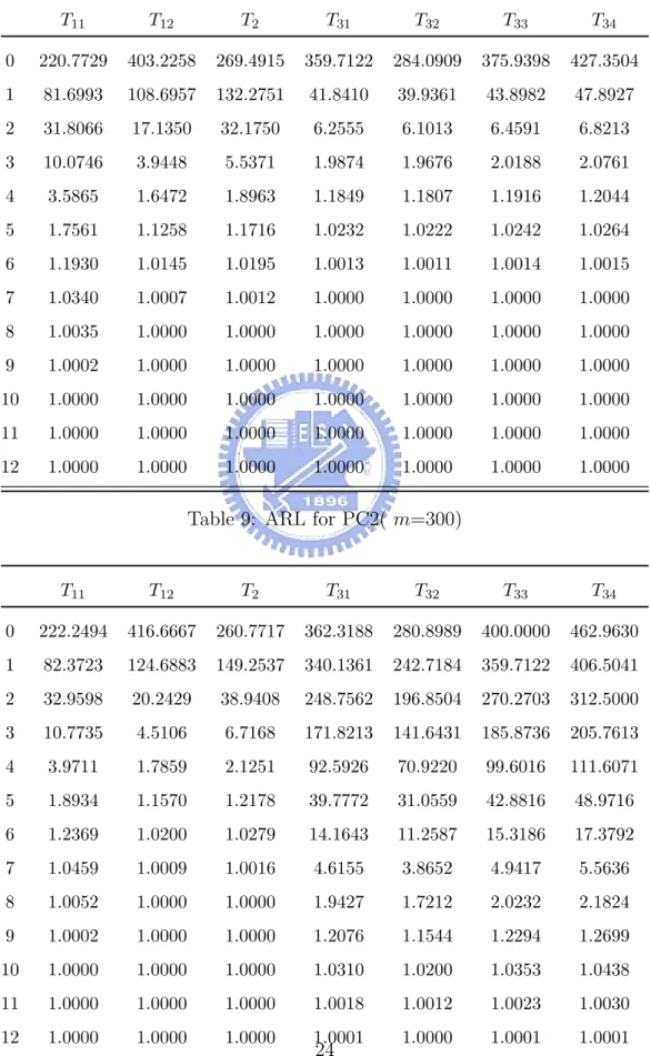
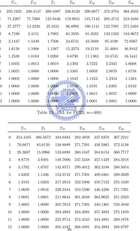
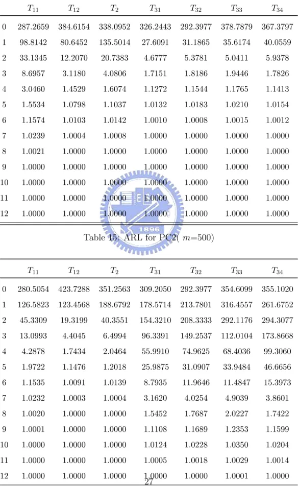
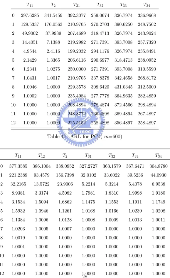
Tables 5-19 show the ARL values when eigenvalues and eigenvectors need to be esti-mated from historical m profiles. The corresponding power curves are given in Figures 7-21. The results of this simulation study are summarized as below:

• For m not large enough, the ARL0 of all the T2 charts are disired This indicates the

estimation error does play an important role in the performance of the charts. We would need a fairly large historical data set to get the estimation accurate enough.

(27)

• For the T2 _{charts, the one using only effective components has ARL}

0 values closer

to 370.4, then the one using all components. The former also has a better detecting power than the latter.

• Again, the performance of the combined chart falls in between the two T2 _chart.

• As to the TSS chart, using sample eigenvalues to construct the control limit (T33)

has ARL0 value than the one using the “true” control limit (T31). In fact, they are

not too far from the nominal value of 370.4. This indicates that this chart (T33) may

be useful in practice.

5 Conclusion

In recent years, the profile monitoring has become a popular area of research in statistical process control. In this study, we discuss profile monitoring schemes with nonparametric regression models. We use the principal components analysis to analyze the covariance structure of the profiles and use the principal component scores that capture special fea-tures of profiles for process monitoring.

In the thesis, we compare three statistics. The first statistic is the usual T2. T2 treats each principal component equally important but has poor power with an increasing the number of principal components. Thus, we only select the first K principal components according the proportion of the variation they explain. The second statistic is the max-imum score, which corresponds to the combined chart that combines all the PC score charts. It monitors each component of a profile and also treats each principal component equally important. The third statistics is the TSS. It is sensitive to “important” principal components and insensitive to the “unimportant” principal components.

(28)

However, the effects of shifts on those components with little contribution to the overall profile may be statistically significant but in fact have no practical significance in quality. Wasting some power on “unimportant” components, classical T2 statistics have less power in detecting changes in the “important” component. On the other hand, the statistic we propose giving more weights to more “important”principal components scores is sensitive to the change of the “important” principal components. Then, when shifts occur in the “important” principal component, the statistic we propose can detect more quickly than classical T2 _{statistics. It is very insensitive to those “unimportant” components since}

almost no weights are given to them.

However, our simulation shows TSS only performs well in PC1, the power of TSS decreases very quickly after PC2. It has almost no power for PC3 and on. This is because the eigenvalues of the VDP data drop so quickly from. λ1=0.8451 to λ2=0.1076, then to

λ3=0.0192, and so on. It seems the weights need to be adjusted if the process changes

are bound to be captured by some principal components other than PC1. This could be a potential future research topic.

(29)

References

[1] Anderson, T. W. (2003). An Introduction to Multivariate Statistical Analysis, 3rd, edition. Wiley, New York.

[2] Castro, P. E., Lawton, W. H., and Sylvester, E. A. (1986). “Principal Models of Variation for Processes With Continuius Sample Curves”. Technormetrics 28, pp. 329-337.

[3] Jensen, W. A., Birch, J. B., and Woodall W. H. (2006a). “Profile Monitoring via Nonlinear Mixed Models”, Techniquical Report. Virginia Polytechnic Institute and State University.

[4] Jensen, W. A., Jones-Farmer, L. A., Champ, C. W., and Woodall W. H. (2006b).“Effects of Parameter Estimation on Control Chart Properties: A Litera-ture Review”,Journal of Quality Technology 38, pp. 349-366.

[5] Kang, L. and Albin, S. L. (2000).“On-Line Monitoring when the Process Yields a Linear Profile”. Journal of Quality Technology 32, pp. 418-426.

[6] Kim, K., Mahmoud, M. A., and Woodal, W. H. (2003).“On the Monitoring of Linear Profiles”. Journal of Quality Technology 35, pp. 317-328.

[7] Mestek, O., Pavlik, J., and Suchanek, M. (1994). “Multivariate Control Charts: Con-trol Charts for Calibration Curves”. Fresenius Journal of Analytical Chemistry 350, pp. 344-351.

[8] Rice, J. A. and Silverman, B. W. (1991) “Estimating the Mean and Covariance Struc-ture Nonparametrically When the Data Are Curves”. Journal of the Royal Statistical Society, Ser. B, 53, pp. 233-243.

[9] Ramsay, J. O. and Silverman, B. W. (2002) Applied Functional Data Analysis: Meth-ods and Case Studies. Springer, New York.

(30)

[11] Satterthwaite, F. W. (1941) “Synthesis of Variance”, Psychometrik, 6, 309-316. [12] Shiau, J.-J. H. and Weng, Z.-P (2004) “Profile Monitoring by Nonparametric

Regres-sion”. Techniqual Report. Institute of Statistics, National Chiao Tung University. [13] Walker, E. and Wright, S. (2002) Comparing Curves Using Additive Models, Journal

of Quality Technology 34, pp. 118-129.

[14] Williams, J. D., Woodall, W. H., and Birch, J. B. (2003), “Phase I Analysis of Non-linear Product and Process Quality Profiles”, Technical Report. Virginia Polytechnic Institute and State University.

[15] Woodall, W. H., Spitzner, D. J., Montgomery, D. C., and Gupta, S. (2004). “Using Control Charts to Monitor Process and Product Quality Profiles”, Journal of Quality Technology 36, pp. 309-320.

(31)

Table 1: Eigenvalues for smoothed VDP data (proportion of explaining variation) k λk k λk k λk 1 899.1265 9 1.6551 17 0.5106 (0.8451) (0.0015) (0.0005) 2 114.4609 10 1.3654 18 0.3880 (0.1075) (0.0012) (0.0003) 3 20.4119 11 1.2072 19 0.3788 (0.0191) (0.0011) (0.0003) 4 9.4104 12 1.0337 20 0.2879 (0.0088) (0.0009) (0.0002) 5 3.2126 3 0.8993 21 0.2800 (0.0030) (0.0008) (0.0002) 6 2.7177 14 0.6758 22 0.2529 (0.0025) (0.0006) (0.0002) 7 2.3202 15 0.6040 23 0.1787 (0.0021) (0.0005) (0.0001) 8 1.9736 16 0.5144 (0.0018) (0.0004)

(32)

Table 2: ARL for PC1 T11 T12 T2 T31 T32 0 370.3703 370.3703 370.3703 370.3703 287.3563 1 217.3913 103.7344 221.2389 45.2488 36.2318 2 60.9756 15.3280 28.4414 6.3259 5.6357 3 14.6842 3.5868 4.9677 2.0023 1.8912 4 4.3821 1.5755 1.7818 1.1791 1.1565 5 1.9051 1.1044 1.1418 1.0222 1.0187 6 1.2214 1.0111 1.0155 1.0014 1.0011 7 1.0384 1.0005 1.0000 1.0000 1.0000 8 1.0037 1.0000 1.0000 1.0000 1.0000 9 1.0002 1.0000 1.0000 1.0000 1.0000 10 1.0001 1.0000 1.0000 1.0000 1.0000 11 1.0000 1.0000 1.0000 1.0000 1.0000 12 1.0000 1.0000 1.0000 1.0000 1.0000

Table 3: ARL for PC2

T11 T12 T2 T31 T32 0 370.3703 370.3703 370.3703 370.3704 287.3563 1 217.3913 103.7344 221.2389 294.1176 242.7184 2 60.9756 15.3280 28.4414 303.0303 238.0952 3 14.6842 3.5860 4.9677 194.5525 143.6781 4 4.3821 1.5755 1.7818 108.4598 80.7754 5 1.9051 1.1044 1.1418 44.6827 33.9673 6 1.2214 1.0111 1.0155 15.8177 12.0569 7 1.0384 1.0005 1.0008 5.25762 4.12269 8 1.0037 1.0002 1.0000 2.0786 1.7925 9 1.0002 1.0000 1.0000 1.2426 1.1713 10 1.0001 1.0000 1.0000 1.0372 1.0227 11 1.0000 1.0000 1.0000 1.0028 1.0014 12 1.0000 1.0000 1.0000 1.0000 1.0000

(33)

Table 4: ARL for PC23 T11 T2 T31 T32 0 370.3703 370.3703 333.3333 260.4166 1 217.3913 221.2389 384.6153 267.3796 2 60.9756 28.4414 381.6793 297.6190 3 14.6842 4.9677 335.5704 268.8172 4 4.3821 1.7818 406.5040 292.3976 5 1.9051 1.1418 406.5040 335.5704 6 1.2214 1.0155 387.5968 292.3976 7 1.0384 1.0008 359.7122 260.4166 8 1.0037 1.0000 359.7122 268.8172 9 1.0002 1.0000 373.1343 277.7777 10 1.0001 1.0000 387.5968 284.0909 11 1.0000 1.0000 359.7122 287.3563 12 1.0000 1.0000 347.3152 288.14523

Table 5: ARL for PC1( m=200)

T11 T12 T2 T31 T32 T33 T34 0 155.3097 236.9668 112.4590 214.5922 263.1578 367.6470 256.4102 1 34.4827 58.7544 74.9625 24.5700 36.6300 35.5114 28.1056 2 13.8927 9.96618 16.6444 4.3335 5.7730 5.4042 4.6576 3 5.2675 2.8088 3.7147 1.6500 1.9043 1.8492 1.7088 4 2.3243 1.4020 1.5549 1.1160 1.1671 1.1584 1.1281 5 1.3730 1.0685 1.0948 1.01268 1.0209 1.0189 1.0144 6 1.0842 1.0060 1.00888 1.0006 1.0011 1.0004 1.0006 7 1.0116 1.0002 1.0003 1.0000 1.0000 1.0002 1.0002 8 1.0008 1.0000 1.0000 1.0000 1.0000 1.0000 1.0000 9 1.0002 1.0000 1.0000 1.0000 1.0000 1.0000 1.0000 10 1.0000 1.0000 1.0000 1.0000 1.0000 1.0000 1.0000

(34)

Table 6: ARL for PC2( m=200) T11 T12 T2 T31 T32 T33 T34 0 154.9451 235.8491 114.4165 201.6129 274.7253 337.8378 228.3105 1 40.2901 81.1688 88.0282 188.6792 265.9574 335.5705 226.2443 2 16.8237 13.5355 24.5459 153.8462 234.7418 264.5503 182.4818 3 6.0518 3.4729 5.1020 102.8807 149.2537 177.9359 125.6281 4 2.5431 1.5520 1.8230 58.6166 84.4595 104.6025 71.2251 5 1.4504 1.1000 1.1514 26.8528 37.3692 47.1698 32.4675 6 1.1048 1.0107 1.0163 9.5475 14.6071 17.0823 11.4784 7 1.0163 1.0006 1.0008 3.3697 4.8866 5.6218 3.9364 8 1.0014 1.0000 1.0000 1.6070 2.0075 2.1865 1.7538 9 1.0001 1.0000 1.0000 1.1237 1.2262 1.2752 1.1630 10 1.0000 1.0000 1.0000 1.0156 1.0345 1.0446 1.0224 11 1.0000 1.0000 1.0000 1.0009 1.0026 1.0036 1.0014 12 1.0000 1.0000 1.0000 1.0000 1.0000 1.0001 1.0001

T11 T2 T31 T32 T33 T34 0 154.1712 236.8224 116.0784 276.4167 364.8780 228.3105 1 39.2157 63.2111 200.0000 294.1176 352.1127 241.5459 2 18.7758 18.1159 196.8504 287.3563 320.5128 227.2727 3 7.3206 4.9796 204.9180 294.1176 352.1127 256.4103 4 3.1504 2.0962 204.0816 306.7485 316.4557 242.7184 5 1.6904 1.2916 206.6116 285.7143 375.9398 247.5248 6 1.1905 1.0657 210.0840 280.8989 384.6154 255.1020 7 1.0371 1.0094 200.0000 304.8780 328.9474 234.7418 8 1.0041 1.0006 195.3125 289.0173 344.8276 227.2727 9 1.0003 1.0000 217.3913 263.1579 333.3333 251.2563 10 1.0000 1.0000 207.2487 251.2884 324.1854 228.2159 11 1.0000 1.0000 219.1488 285.1587 334.7575 258.6783

(35)

T11 T12 T2 T31 T32 T33 T34 0 222.2494 416.6667 260.7717 362.3188 280.8989 400.0000 462.9630 1 82.3723 124.6883 149.2537 340.1361 242.7184 359.7122 406.5041 2 32.9598 20.2429 38.9408 248.7562 196.8504 270.2703 312.5000 3 10.7735 4.5106 6.7168 171.8213 141.6431 185.8736 205.7613 4 3.9711 1.7859 2.1251 92.5926 70.9220 99.6016 111.6071 5 1.8934 1.1570 1.2178 39.7772 31.0559 42.8816 48.9716 6 1.2369 1.0200 1.0279 14.1643 11.2587 15.3186 17.3792 7 1.0459 1.0009 1.0016 4.6155 3.8652 4.9417 5.5636 8 1.0052 1.0000 1.0000 1.9427 1.7212 2.0232 2.1824 9 1.0002 1.0000 1.0000 1.2076 1.1544 1.2294 1.2699 10 1.0000 1.0000 1.0000 1.0310 1.0200 1.0353 1.0438

(36)

Table 10: ARL for PC23( m=300) T11 T2 T31 T32 T33 T34 0 225.3132 286.5671 381.2048 276.2430 402.5806 389.7122 1 82.3723 83.6120 312.5488 297.6190 328.9473 373.1343 2 24.5218 15.0966 324.6753 280.8984 337.8378 373.1343 3 8.2877 3.9491 342.4657 322.5806 359.7122 403.2258 4 2.9751 1.6767 349.6503 299.4011 373.1343 423.7288 5 1.5691 1.1436 328.9473 289.0173 354.6099 403.2255 6 1.1336 1.0203 364.9635 261.7801 375.9398 409.8360 7 1.0209 1.0015 375.9398 303.0303 393.7007 442.4778 8 1.0017 1.0001 316.4556 279.3296 340.1360 400.5156 9 1.0000 1.0000 328.4822 289.4891 348.5842 431.0344 10 1.0000 1.0000 357.8843 236.8997 316.1584 403.5941 11 1.0000 1.0000 318.2562 289.4879 369.4988 389.2971 12 1.0000 1.0000 316.158 325.5498 365.2594 408.4997

T11 T12 T2 T31 T32 T33 T34 0 222.2494 324.2152 374.2160 340.4494 274.7253 352.1127 374.8252 1 82.3723 53.5906 92.4214 20.4666 23.3333 33.2882 41.6967 2 32.9598 8.9977 14.6413 3.8772 4.2676 5.9552 5.2827 3 10.7735 2.5788 3.2757 1.5708 1.8194 1.9418 1.6448 4 3.9711 1.3339 1.4532 1.0989 1.1498 1.1763 1.1137 5 1.8934 1.0537 1.0739 1.0102 1.0172 1.0218 1.0122 6 1.2369 1.0080 1.0111 1.0006 1.0009 1.0012 1.0007 7 1.0459 1.0002 1.0005 1.0000 1.0001 1.0000 1.0000 8 1.0052 1.0000 1.0000 1.0000 1.0000 1.0000 1.0000 9 1.0002 1.0000 1.0000 1.0000 1.0000 1.0000 1.0000 10 1.0002 1.0000 1.0000 1.0000 1.0000 1.0000 1.0000 11 1.0002 1.0000 1.0000 1.0000 1.0000 1.0000 1.0000

(37)

T11 T2 T31 T32 T33 T34 0 354.4165 386.5672 334.0483 282.4859 337.8378 367.2241 1 76.6871 83.6120 138.8889 271.7391 438.5965 372.4138 2 28.3607 15.0966 133.6898 260.4167 384.6154 360.7717 3 8.8778 3.9491 149.7006 247.5248 357.1429 284.5018 4 3.1702 1.6767 142.8571 299.4012 362.3188 280.5054 5 1.6202 1.1436 153.3742 271.7391 409.8361 289.3939 6 1.3185 1.0203 217.3913 322.5806 359.7122 255.1020 7 1.0639 1.0016 239.2344 310.5590 446.4286 271.7391 8 1.0081 1.0001 211.8644 301.2048 364.9635 251.2563 9 1.0005 1.0000 205.7613 271.7391 340.1361 250.4840 10 1.0000 1.0000 283.4983 284.4985 357.4894 275.1859

(38)

T11 T12 T2 T31 T32 T33 T34 0 280.5054 423.7288 351.2563 309.2050 292.3977 354.6099 355.1020 1 126.5823 123.4568 188.6792 178.5714 213.7801 316.4557 261.6752 2 45.3309 19.3199 40.3551 154.3210 208.3333 292.1176 294.3077 3 13.0993 4.4045 6.4994 96.3391 149.2537 112.0104 173.8668 4 4.2878 1.7434 2.0464 55.9910 74.9625 68.4036 99.3060 5 1.9722 1.1476 1.2018 25.9875 31.0907 33.9484 46.6656 6 1.1535 1.0091 1.0139 8.7935 11.9646 11.4847 15.3973 7 1.0232 1.0003 1.0004 3.1620 4.0254 4.9039 3.8601 8 1.0020 1.0000 1.0000 1.5452 1.7687 2.0227 1.7422 9 1.0001 1.0000 1.0000 1.1108 1.1689 1.2353 1.1599 10 1.0000 1.0000 1.0000 1.0124 1.0228 1.0350 1.0204 11 1.0000 1.0000 1.0000 1.0005 1.0018 1.0029 1.0014

(39)

Table 16: ARL for PC23( m=500) T11 T2 T31 T32 T33 T34 0 297.6285 341.5459 392.3077 259.0674 326.7974 336.9668 1 129.5337 176.0563 210.9705 270.2703 390.6250 248.7562 2 49.9002 37.9939 207.4689 318.4713 326.7974 243.9024 3 14.4051 7.1388 219.2982 271.7391 393.7008 257.7320 4 4.9544 2.4116 199.2032 294.1176 326.7974 235.8491 5 2.1429 1.3365 206.6116 290.6977 318.4713 238.0952 6 1.2341 1.0275 250.0000 271.7391 393.7008 310.5590 7 1.0431 1.0017 210.9705 337.8378 342.4658 268.8172 8 1.0046 1.0000 229.3578 308.6420 431.0345 312.5000 9 1.0002 1.0000 235.4984 277.7778 364.9635 282.4859 10 1.0000 1.0000 208.4894 278.4874 372.4566 298.4894 11 1.0000 1.0000 248.8772 236.4898 369.4894 267.4897 12 1.0000 1.0000 225.5152 258.4898 356.4897 258.4897

T11 T12 T2 T31 T32 T33 T34 0 377.3585 386.1004 338.0952 327.2727 363.1579 367.6471 304.8780 1 221.2389 93.4579 156.7398 32.0102 33.6022 39.5236 44.0930 2 32.2165 13.5722 23.9006 5.2214 5.3214 5.4078 6.9538 3 8.9381 3.3174 4.5082 1.7981 1.8310 1.9998 1.9180 4 3.1534 1.5094 1.6862 1.1475 1.1553 1.1911 1.1749 5 1.5932 1.0946 1.1261 1.0168 1.0166 1.0239 1.0208 6 1.1384 1.0096 1.0128 1.0008 1.0009 1.0013 1.0011 7 1.0203 1.0005 1.0007 1.0000 1.0000 1.0000 1.0000 8 1.0019 1.0000 1.0000 1.0000 1.0000 1.0000 1.0000 9 1.0001 1.0000 1.0000 1.0000 1.0000 1.0000 1.0000 10 1.0000 1.0000 1.0000 1.0000 1.0000 1.0000 1.0000

(40)

Table 19: ARL for PC23(m=600)

T11 T2 T31 T32 T33 T34 0 375.9398 326.2443 325.2252 384.0909 340.1361 385.7143 1 210.9705 147.9290 232.5581 320.5128 354.6099 310.5590 2 40.6174 27.0856 221.2389 287.3563 373.1343 310.5590 3 12.3365 5.2598 231.4815 265.9574 387.5969 310.5590 4 4.0700 1.8858 233.6449 265.9574 347.2222 299.4012 5 1.8669 1.1814 208.3333 312.5000 314.4654 273.2240 6 1.2212 1.0236 227.2727 271.7391 367.6471 312.5000 7 1.0398 1.0018 226.2443 273.2240 370.3704 322.5806 8 1.0046 1.0000 209.2050 273.2240 359.7122 290.6977 9 1.0001 1.0000 236.9668 255.1020 384.6154 314.4654 10 1.0000 1.0000 286.4894 225.7587 357.5278 323.7755 11 1.0000 1.0000 254.4568 279.5630 324.7858 312.5278

(41)

0.0 0.1 0.2 0.3 0.4 0.5 0.6 0.7 35 40 45 50 55 60 65 Depth Density

Figure 1: Original 24 VDP-profiles

0.0 0.1 0.2 0.3 0.4 0.5 0.6 40 45 50 55 60 Smooth VDP 0 0

(42)

● 0 1000 2000 3000 4000 0.0000 0.0004 0.0008 0.0012 Density T3 c*Chisq(df)

(43)

● 0 2 4 6 8 10 12 0.0 0.2 0.4 0.6 0.8 1.0 Power for PC1 shift Power ● ● ● ● ● ● ● ● ● ● ● ● ● ● ● ● ● ● ● ● ● ● ● ● ● ● ● ● T11 T12 T2 T31 T32

Figure 4: Power of PC1 (true VDP)

Figure 5: Power of PC2 (true VDP)

(44)

● 0 2 4 6 8 10 12 0.0 0.2 0.4 0.6 0.8 1.0 Power for PC1 (m=200) shift Power ● ● ● ● ● ● ● ● ● ● ● ● ● ● ● ● ● ● ● ● ● ● ● ● ● ● ● ● ● ● ● ● ● ● ● ● ● ● ● ● ● ● ● ● ● T11 T12 T2 T31 T32 T33 T34

Figure 7: Power for PC1 with m=200

● 0 2 4 6 8 10 12 0.0 0.2 0.4 0.6 0.8 1.0 Power for PC23 (m=200) shift Power ● ● ● ● ● ● ● ● ● ● ● ● ● ● ● ● ● ● ● ● ● ● ● ● ● ● ● ● ● ● T11 T2 T31 T32 T33 T34

(45)

(46)

(47)

(48)

● 0 2 4 6 8 10 12 0.0 0.2 0.4 0.6 0.8 1.0 Power for PC2(m=600) shift Power ● ● ● ● ● ● ● ● ● ● ● ● ● ● ● ● ● ● ● ● ● ● ● ● ● ● ● ● ● ● T11 T12 T2 T31 T32 T33

利用主成份分析監控剖面資料之研究

國

立

交

通

大

學

統計學研究所

碩

士

論

文

利用主成份分析監控剖面資料之研究

Profile Monitoring via Principal Components

研 究 生：王筱娟

指導教授：洪志真 博士

利用主成份分析監控剖面資料之研究

Profile Monitoring via Principal Component

研 究 生：王筱娟 Student：Hshiao-Chuan Wang

指導教授：洪志真 Advisor：Jyh-Jen Horng Shiau

國 立 交 通 大 學

統計學研究所

碩 士 論 文

誌

謝

兩年的碩士班生涯即將結束，馬上就要走入人生另一個旅程，

利用主成份分析監控剖面資料之研究

研究生：王筱娟 指導教授：洪志真博士

國立交通大學統計學研究所

摘要

Profile Monitoring via Principal Components

Student: Hshiao-Chuan Wang

Advisor: Jyh-Jen Horng Shiau

Institute of Statistics

National Chiao Tung University

Hsinchu, Taiwan

Contents

List of Tables

List of Figures

1

Introduction

2

Review on Background Methodologies

2.1

Nonparametric Regression

2.2

Functional Data Analysis

2.3

Principal Components Analysis

2.4

Functional PCA vs. PCA

3

Monitoring Schemes

3.1

Monitoring Statistics

3.2

Control Limits

4

Simulation Studies

4.1

Data Generation

4.2

Number of Principal Components

4.3

Simulation Results

5

Conclusion

References

研究生：王筱娟

指導教授：洪志真博士

研究生：王筱娟 Student：Hshiao-Chuan Wang

國立交通大學

碩士論文

研究生：王筱娟指導教授：洪志真博士