基於類神經網路的演化策略應用於一階動態系統

全文

(1)國立交通大學電機與控制工程學系碩士論文. 基於類神經網路的演化策略應用於一階動態系統. Neural Network-Based Evolution Strategies for Implementing First Order Dynamic Systems. 研究生：陳思穎. A. 指導教授：陳永平教授. 中華民國九十六年六月.

(2) 基於類神經網路的演化策略應用於一階動態系統 Neural Network-Based Evolution Strategies for Implementing First Order Dynamic Systems. 研究生：陳思穎. Student：Sze-Ying Chen. 指導教授：陳永平. Advisor：Yon-Ping Chen. 國立交通大學電機與控制工程學系碩士論文. A Thesis Submitted to Department of Electrical and Control Engineering College of Electrical and Computer Engineering National Chiao Tung University in Partial Fulfillment of the Requirements for the Degree of Master in Electrical and Control engineering June 2007 Hsinchu, Taiwan, Republic of China. 中華民國九十六年六月.

(3) 基於類神經網路的演化策略應用於一階動態系統. 學生：陳思穎. 指導教授：陳永平博士. 國立交通大學電機與控制工程學系. 摘要 Chinese Abstract 本論文目的在於利用類神經網路學習一階動態系統，用以控制一迴授系統。論文 3.2 節中，為了學習一階動態系統，提出兩種簡單的類神經網路架構，一種是一般的類神經網路，另一種加入了參數影響，而此參數是根據一階差分方程而來的。另外，本論文不用常見的倒傳遞學習法則，而用一演化策略，因為倒傳遞學習法則必須知道反向動態系統，但反向動態系統並不容易得到，而該演化策略並無此缺點。雖然使用該演化策略的學習時間較長，但類神經網路經過演化策略的學習後，能表現的跟目標系統極度相似，即使將此類神經網路放入一有外來雜訊的迴授系統當控制器時，亦能控制系統穩定不受雜訊影響。. i.

(4) Neural Network-Based Evolution Strategies for Implementing First Order Dynamic Systems. Student: Sze-Ying Chen. Advisor: Dr. Yon-Ping Chen. Department of Electrical and Control Engineering National Chiao Tung University. ABSTRACT English Abstract The objective of the thesis is training a neural network to perform as a first order LTI system, and then apply as a controller. Based on evolution strategies and the first order difference equation, two simple neural network structures are designed to implement the first order LTI systems. With the evolution strategies, it is not necessary to know the inverse dynamic system, which is required while using the backpropagation learning algorithm in general neural networks. From the simulation results, the proposed neural networks, called general structure (GS) and structure with sampling time (SST), may perform almost the same as the first order LTI system and are robust to an unexpected disturbance as a controller, even though the learning time is long. ii.

(5) Acknowledgement. 轉瞬間，碩士生涯就要結束了。回想這兩年，每當研究愈深入，愈覺自身之不足，愈覺學海之無涯，幸得指導老師陳永平老師孜孜不倦的教導，讓論文能順利完成。老師除了在研究上給予建議與指導外，對於研究方法與學習態度也相當重視，更提供許多英文能力的訓練，讓我們除了專業上的深入外，有更多其他方面的成長，僅向老師至上最誠摯的謝意與感念。同時，謝謝口試委員張浚林學長及梁耀文老師寶貴的建議與指教，讓論文得以更加完善。其次，也要感謝一路支持我的父母兄長，還有一路陪伴我的朋友麗中、欣宜、依文、君如、心韻，我能度過低潮，堅持到現在，都要歸功於您們。最後，要謝謝實驗室伙伴胤宏、士昌、子揚、坤佑的加油打氣，以及實驗室世宏學長、建峰學長和桓展學長的指教，還要謝謝這一年來相伴的學弟妹們，由於你們，讓平凡的研究生活更點綴了許多歡笑的回憶。僅以此篇論文獻給所有關心、照顧我的人。. 陳思穎 2007.07.03. iii.

(6) Contents. Chinese Abstract................................................................................................... i English Abstract ..................................................................................................ii Acknowledgement ..............................................................................................iii Contents............................................................................................................... iv List of Figures ..................................................................................................... vi List of Tables .....................................................................................................viii Notation ............................................................................................................... ix. Chapter 1 Introduction ....................................................................................... 1 Chapter 2 Intelligent Control............................................................................. 3 2.1. Introduction to Neural Network .......................................................... 3. 2.2. Neural Network for Control ................................................................. 8. Chapter 3 Evolution Strategies ........................................................................ 15 3.1. Modeling of First Order LTI System................................................. 15. 3.2. Neural Network Structure .................................................................. 18. 3.2.1 3.2.2 3.2.3. 3.3. Structure for The First Order Difference Equation ....................................18 General Structure ...........................................................................................19 Structure with Sampling Time ......................................................................21. Evolution Strategies............................................................................. 22. 3.3.1 3.3.2 3.3.3 3.3.4 3.3.5. Initial Individuals Creation ...........................................................................24 Reproduction Process.....................................................................................25 Learning Process.............................................................................................28 Elite Process ....................................................................................................30 Flow Chart ......................................................................................................33 iv.

(7) Chapter 4 Simulation Results........................................................................... 34 4.1. Influence of The Sampling Time ........................................................ 35. 4.2. Influence of The Initial Weights Setting............................................ 49. 4.3. Implement as a Controller.................................................................. 55. 4.3.1 4.3.2. System with First Order LTI Plant ...............................................................56 System with Second Order LTI Plant ...........................................................58. Chapter 5 Conclusion........................................................................................ 62 References .......................................................................................................... 64. v.

(8) List of Figures. Figure 2.1 An artificial neuron ...................................................................................................4 Figure 2.2 Multilayer feedforward network ...............................................................................5 Figure 2.3 two-layer back-propagation network ........................................................................6 Figure 2.4 the feedback system ..................................................................................................8 Figure 2.5 to train neural network plant .....................................................................................9 Figure 2.6 to train the neural network controller......................................................................10 Figure 2.7 the fully recurrent neural network........................................................................... 11 Figure 3.1 the first order difference equation using one neuron ..............................................19 Figure 3.2 the GS for first order LTI system ............................................................................20 Figure 3.3 the SST for first order LTI system ..........................................................................22 Figure 3.4 Illustration of finding children inward ....................................................................26 Figure 3.5 Illustration of finding children outward ..................................................................27 Figure 3.6 Random children creation .......................................................................................27 Figure 3.7 finding temporal individual of the next step ...........................................................29 Figure 3.8 the flow chart of the evolution strategies ................................................................33 Figure 4.1.1 the learning result of the GS under sampling time 0.01.......................................36 Figure 4.1.2 the change of the sum of the error of the GS under sampling time 0.01 .............36 Figure 4.2.1 the learning result of the SST under sampling time 0.01 .....................................37 Figure 4.2.2 the change of the sum of the error of the SST under sampling time 0.01............37 Figure 4.3.1 the learning result of the GS under sampling time 0.001.....................................38 Figure 4.3.2 the change of the sum of the error of the GS under sampling time 0.001 ...........38 Figure 4.4.1 the learning result of the SST under sampling time 0.001 ...................................39 Figure 4.4.2 the change of the sum of the error of the SST under sampling time 0.001..........39 Figure 4.5.1 testing result when initial condition y(0) is 0.5....................................................42 Figure 4.5.2 testing result when initial condition y(0) is 2.......................................................43 Figure 4.5.3 testing result when initial condition y(0) is -2 .....................................................43 Figure 4.6.1 testing result when input function u = 2p(t).........................................................44 Figure 4.6.2 testing result when input function u = -2p(t)........................................................44 Figure 4.6.3 testing result when input function u = sin(2t) ......................................................45 Figure 4.7 the testing result with ..............................................................................................46 Figure 4.8 the testing result with ∆ T =0.001 of the learned neural network with ∆ T =0.01 46 Figure 4.9 the learning result of the SST with sampling time 0.01, 0.001, 0.0001..................47 Figure 4.10.1 the testing result under the sampling time smaller than trained sampling time .48 Figure 4.10.2 the testing result under the sampling time between trained sampling time .......48 Figure 4.10.3 the testing result under the sampling time larger than trained sampling time ...49 vi.

(9) Figure 4.11.1 the learning result of the GS under sampling time 0.001...................................51 Figure 4.11.2 the change of the sum of the error of the SST under sampling time 0.001........51 Figure 4.12.1 testing result when initial condition y(0) is 0.5..................................................52 Figure 4.12.2 testing result when initial condition y(0) is 2.....................................................53 Figure 4.12.3 testing result when initial condition y(0) is -2 ...................................................53 Figure 4.13.1 testing result when input function u = 2p(t) .......................................................54 Figure 4.13.2 testing result when input function u = -2p(t)......................................................54 Figure 4.13.3 testing result when input function u = sin(2t) ....................................................55 Figure 4.14 the feedback system ..............................................................................................56 Figure 4.15 the learning result of a controller: u& (t ) + 6.5 u (t ) = 2.5 e(t ) ..................................56. Figure 4.16 the testing result of the feedback system with a neural network controller ..........57 Figure 4.18 the testing result of the feedback system with unexpected disturbance................58 Figure 4.19 the feedback system ..............................................................................................58 Figure 4.20 the testing result of the feedback system with a neural network controller ..........59 Figure 4.21 the feedback controller with disturbance ..............................................................60 Figure 4.22 the testing result of the feedback system with unexpected disturbance................60. vii.

(10) List of Tables Table 4.1 the results of learning with different sampling times ...............................................40 Table 4.2.1 the error and the accurate rate of learning with sampling time 0.01 .....................40 Table 4.2.2 the error and the accurate rate of learning with sampling time 0.001 ...................41 Table 4.3 learning results of GS with sampling time 0.001 .....................................................50. viii.

(11) Notation. GS. : General structure. SST. : Structure with sampling time. Wkg. : The kth individual of the gth generation. ng. : The number of the individuals in the gth generation. l. : The multiple of the distance in the reproduction process. Ω kg (s ). : The kth child of the sth step in the gth generation. Ωtmp(s) : The temporal individual of the sth step δΩ(s). : The difference of the sth step. δΩ ⊥ (s ) : The perpendicular vector of δW(s) δΩtmp(s) : The temporal difference of the sth step. ix.

(12) Chapter 1 Introduction. In recent years, many researchers have been devoted to developing intelligent theories, such as fuzzy logic [1], genetic algorithm [2-4], and neural network theory [5, 6]. These intelligent theories are used in more and more fields [7, 8] and show their great power as a problem solver. Many investigators have developed intelligent machines, such as Kismet and Aryan. We also built an eye-robot to mimic the motion of human eyes, and try to control the robot. In the conventional control theory, the model of the plant should be known exactly before designing the controller. If the model has some error from the real system, the designed controller may not stable and control well. However, in reality, many plants are complex and the model could not be determined, thus that restricts the use of the conventional control theory. The controller could not be designed by the conventional control theory when the model of the plant is uncertain. Fortunately, the intelligent control needs no exact model of the plant to design a controller, and can learn to control the system gradually. Thus, the restriction of the conventional control theory is the reason why we use the intelligent theory to control our robot. Basically, the artificial neural network based on the human neural network contains many neurons connected with synaptic weights. Thus, it can learn, recall, and generalize from training data like a human brain. Models of the neurons, models of the structure and the learning algorithm are the basic entities of the artificial neural network. They play important. 1.

(13) roles in calculation of the output. Some learning algorithms focus on changing the way of the connections between neurons [11], some focus on adjusting the connecting weights [12], and some focus on the above two simultaneously [13]. One the other hand, the learning of the neural network theory could be divided into three main parts: supervised learning, unsupervised learning, and reinforcement learning [14]. The objective of the algorithm is to approach the optimal value of its error function. If the accurate data exist, the supervised learning is easier to approach the optimal value of the error function than the other two, because it doesn’t view a wrong result as correct. In the thesis, we focus on adjusting the connecting weight by supervised learning in system control field. Although backpropagation learning algorithm is commonly used and easy to apply, it has a problem of local optimization [15]. Hence, evolution strategies are used to increase the search space and thus try to avoid local optimization. The thesis contains five chapters. The introduction is described in this chapter. Chapter 2 describes the basic neural network theory and some application in system control. The learning algorithms for neural network, evolution strategies, are explained in detail in Chapter 3 and the simulation results are demonstrated in Chapter 4. Finally, the conclusion is given in Chapter 5.. 2.

(14) Chapter 2 Intelligent Control. Intelligent control designed to simulate intelligent biological systems is a new control method which combines automatic control and artificial intelligence. The processes of the machines using intelligent control will be similar with the human thinking. Today automatic control systems have played an important role of our daily life, such as airplanes and spacecrafts. Although automatic control has works well, it is difficult to design a controller for a complex dynamic system. To solve the problem, recently investigators have paid their attentions to the intelligent algorithms, such as fuzzy theory and neural network, to achieve the system identification and controller design. It is known that neural networks are modeled after the physical architecture of the human brain; therefore, this chapter will focus on the control using neural network, which has been widely applied to intelligent systems.. 2.1 Introduction to Neural Network Neural networks demonstrate the ability to learn, recall, and generalize from training patterns or data. In general, the biological neural network in human brain is constructed by a large amount of neurons, which contain somas, axons, dendrites, and synapses. The current excited by the impulse from the other neuron will change the strength of synapses until steady when the biological neural network is learning. Artificial neural networks (ANN) which are. 3.

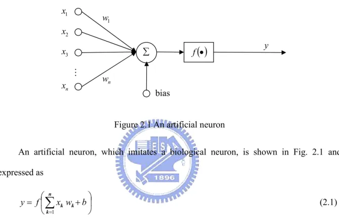
(15) modeled after the physical architecture of the human brain is proposed to simulate the learning function for intelligent machine. Therefore, ANN is highly interconnected by a large of processing elements, which are also called artificial neuron or neuron simply, and its connective behavior is like human brain. x1. w1. x2. xn. f (•). ∑. x3 M. y. wn bias Figure 2.1 An artificial neuron. An artificial neuron, which imitates a biological neuron, is shown in Fig. 2.1 and expressed as ⎛ n ⎞ y = f ⎜ ∑ xk wk + b ⎟ ⎝ k =1 ⎠. (2.1). where the output y is a function of the input xk, k=1,2,3,…. Note that the bias b and the weights wk, k=1,2,3,… are all constant. There are many types of activation function f, linear or nonlinear, and the hyperbolic tangent function described as f ( x ) = tanh ( x ) =. e x − e− x e x + e− x. (2.2). is commonly used. Because ANN is highly interconnected by a large of processing elements, the connection geometry among the processing elements is important to form a ANN. ANN can be constructed by artificial neurons in different modes, such as the commonest multilayer. 4.

(16) feedforward network shown in Fig. 2.2, which possesses one input layer, one output layer and some hidden layers. input. output. M. M. output layer input layer. second hidden layer. first hidden layer Figure 2.2 Multilayer feedforward network The most important element of ANN is the learning rules, which are mainly classified into the parameter learning and the structure learning. The parameter learning is updating the weights in the neural network, while the structure learning is changing the network structure, such as the number of neurons and their connection. It is known that there are three types of parameter learning, including supervised learning, reinforcement learning, and unsupervised learning. In this thesis, the simulation uses a known plant and designed controller, so the input-output pairs of the controller can be gotten easily. The neural network learns the behavior of the controller by using these input-output pairs, and this kind of learning belongs to supervised learning. This thesis will focus on the supervised learning. In supervised learning, the back propagation learning algorithm, based on the simple gradient algorithm for updating the weights, is commonly used in most applications. The back propagation learning is often executed by multilayer feedforward networks with elements containing differentiable activation functions. Such networks are also called the back-propagation networks and Fig. 2.3 shows a back-propagation network consisting of one. 5.

(17) input layer with m neurons, one single hidden layer with l neurons, and one output layer with n neurons. z1 x1. y1. M. M vqj. xj. M. vq1 zq. w1q. vqm. wnq. M wiq. yi. M. M. xm. yn. zl. Figure 2.3 two-layer back-propagation network For. the. z = [z1. back-propagation. network. z2 L zl ] , and y = [ y1 T. in. Fig.. 2.3,. let. x = [x1. x2 L xm ] , T. y2 L yn ] be the inputs of the network, the T. outputs of neurons in the hidden layer, and the outputs of the network, respectively. Let vqj be the weight from the j-th neuron in the input layer to q-th neuron in the hidden layer. and wiq be the weight from the q-th neuron in the hidden layer to i-th neuron in the output layer. Then, the output of the q-th neuron in the hidden layer is described as ⎞ ⎛ m zq = f z ⎜⎜ ∑ vqj x j ⎟⎟ q = 1,2,..., l ⎠ ⎝ j =1. (2.3). where fz is the activation function, and the output of the i-th neuron in the output layer is described as ⎞ ⎛ l yi = f y ⎜⎜ ∑ wiq zq ⎟⎟ i = 1,2,..., n ⎠ ⎝ q =1. (2.4). where fy is the activation function.. 6.

(18) In supervised learning with the given input-output training data (x, d), the cost function is defined as the following error function ⎛ l ⎞⎤ 1 n 1 n ⎡ 2 E (w ) = ∑ (d i − yi ) = ∑ ⎢di − f y ⎜⎜ ∑ wiq zq ⎟⎟⎥ 2 i =1 2 i =1 ⎢⎣ ⎝ q =1 ⎠⎥⎦. 2. (2.5). where yi is the output of the network and di is the desired output. Then, according to the gradient-descent method, the changes of the weights are determined as ∆wiq = − η. ∂E ∂ E ∂ yi = −η ∂ wiq ∂ yi ∂ wiq. ⎡ ⎛ l ⎞⎤ = η(d i − yi )⎢ f y′⎜⎜ ∑ wiq z q ⎟⎟⎥ z q ⎢⎣ ⎝ q =1 ⎠⎥⎦ = ηδoi z q. (2.6). and n ⎛ ∂E ∂ E ∂ yi ∂ z q ⎞⎟ = − η∑⎜ ⎜ ⎟ ∂ vqj i =1 ⎝ ∂ yi ∂ z q ∂ vqj ⎠ n ⎡ ⎞ ⎞ ⎤ ⎛ m ⎛ l = η ∑ ⎢(d i − yi ) f y′⎜⎜ ∑ wiq z q ⎟⎟ wiq ⎥ f z′⎜⎜ ∑ vqj x j ⎟⎟ x j i =1 ⎢ ⎠ ⎠ ⎥⎦ ⎝ j =1 ⎝ q =1 ⎣ = ηδhq x j. ∆vqj = − η. (2.7). ⎡ ⎛ l ⎞n ⎛ m ⎞⎤ where δ oi = (d i − yi )⎢ f y′ ⎜⎜ ∑ wiq z q ⎟⎟⎥ and δhq = f z′⎜⎜ ∑ vqj x j ⎟⎟∑ (δoi wiq ) . Besides, the learning ⎠ i =1 ⎠⎦⎥ ⎝ j =1 ⎣⎢ ⎝ q =1. rate η is often given experimentally to reduce the computing time or increase the precision. Finally, the weights can be updated by ⎧w (n+ 1) = w (n ) + ∆w ⎨ ⎩v (n+ 1) = v (n ) + ∆v. (2.8). It is the advantage that the back propagation algorithm can be used in the networks with nonlinear functions. Many researchers use the simple algorithm to learn classification and. 7.

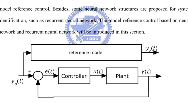
(19) input-output relationship. The objective of this thesis is to control the system using neural network, so the neural network for control will be introduced in the next section.. 2.2 Neural Network for Control Since traditional control theory is based on the mathematic model of the plant, it fails when the mathematic model is unknown or not accurate. The intelligent control theory based on the abilities of thinking and learning of human is not restricted to the mathematic model. It has more abilities to solve the control problem than the conventional control theory. The investigators have proposed many control method based on neural network, such as model reference control. Besides, some neural network structures are proposed for system identification, such as recurrent neural network. The model reference control based on neural network and recurrent neural network will be introduced in this section.. Figure 2.4 the feedback system The model reference control based on neural network is introduced first. When the plant is given, the feedback system is shown as Fig. 2.4 and the controller is the learning objective system [16]. The reference model is designed according to the specification of the problem. Basically, the learning algorithm is based on the gradient method, so the learning process needs two neural networks, one to be a controller and the other to be a plant. This learning can 8.

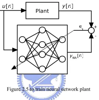
(20) use backpropagation learning algorithm introduced in the last section. To back propagate the error to the neural network, the inverse of the plant should be known. Unfortunately, not every inverse dynamic of the plant exists, or can be known even if it exists. Hence, the neural network plant should be trained first for back propagating the system error to the neural network controller, shown as Fig 2.5. However, it causes that the neural network plant should be retrained whenever the condition of the plant changed a little.. Figure 2.5 to train neural network plant It is known that the learning algorithm alters the connecting weights depending on the error between the plant output and the neural network plant output. If the neural network plant is trained well, it will replace the original plant. It is worthy noticing that the connecting weights of the neural network plant do not change when the neural network controller is trained. Fig. 2.6 shows the learning system for training the neural network controller. Compared with the reference model, the neural network controller does not learn as the real controller. If the plant in s-domain is defined as H(s) and the controller is defined as G(s), the system is described as Y (s ) G (s ) H (s ) = U (s ) 1 + G (s ) H (s ). (2.9). where Y(s) is the system output and U(s) is the system input. However, the neural network 9.

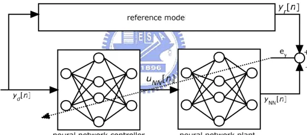
(21) system is described as YNN (s ) = GNN (s ) H NN (s ) U (s ). (2.10). where GNN(s) denotes the neural network controller and HNN (s) denotes the neural network plant. Because the neural network plant is trained as the real plant, HNN (s) is assumed identical to H(s). Thus, the neural network controller does not learn as the real controller, and expressed as GNN (s ) =. G (s ) 1 + G (s ) H (s ). (2.11). which does not equal to G(s).. Figure 2.6 to train the neural network controller The model reference control based on neural network is a simple way to control the system depending on the specification of the problem. However, the neural network plant should be trained first, and that leads errors while the plant changes, such as the input-output relationship and the sampling time. No mater what the plant changes, the neural network plant should be trained again for back propagation precisely. Besides, it is known that the neural. 10.

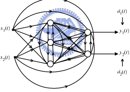
(22) network controller is not the original controller. These restrict the use of the model reference control based on the neural network. Because of the restriction of the inverse dynamic, some investigators proposed other control method without learning the neural network plant [17-19]. For simplicity, the neural network controller could be learned as system identification while the controller is designed, but it can not be guarantee the control ability of the neural network controller. Thus, a fully recurrent neural network, shown as Fig 2.7, is proposed with capability of dynamics and the ability to store the information for later use. In the next paragraph, a leaning algorithm for fully recurrent neural network, real- time recurrent learning (RTRL), will be introduced.. Figure 2.7 the fully recurrent neural network RTRL has been proposed by many investigators independently, and the most used is by Williams and Zipser [20], which is introduced here. The learning algorithms will be described in detail as below. While the network have n neurons, with m external inputs, the outputs of neurons are denoted as ykn(t), kn = 1,2,…,n, and the external inputs are denoted as xki(t), ki = 1,2,…,m,. 11.

(23) where t is the time. These values are concatenated to form the (m+n)-tuple z(t), which is expressed as ⎧ ykn (t ) zk (t ) = ⎨ ⎩ xki (t ). if k = kn. (2.12). if k = n+ ki. which are the outputs of every neurons and input neurons. Since the network is fully connected, the weight matrix W in a n× (m+ n ) matrix to obtain n outputs of neurons by m external inputs and n inputs of neurons. Thus, the net input of the knth neurons at time t can be calculated as skn (t ) = ∑ wknl zl (t ). (2.13). l. where l = 1,2,…,m+n. The output of the neuron at next time step is determined as ykn (t + 1) = f kn (skn (t )) (2.14) where f kn (⋅) is the activation function of the knth neuron. Let the first o neurons exist specified target value d, so the n-tuple error e is described as ⎧d (t ) − ykn (t ) ekn (t ) = ⎨ kn ⎩0. if kn ≤ o otherwise. .. (2.15). Define the overall network error at time t as J (t ) =. 1 [ekn (t )]2 , ∑ 2 kn. (2.16). thus, let J total (t0 ,t1 ) =. t1. ∑ J (t ). (2.17). t = t 0 +1. 12.

(24) denotes the network error running from time t0 to the time t1. W is adjusted along the negative of ∇W J total (t 0 ,t1 ) . Thus, the weight change can be written as. ∆ wij =. t1. ∑ ∆ w (t ). (2.18). ij. t =t 0 +1. where. ∆ wij (t ) = −α. ∂ J (t ) ∂ y (t ) = α ∑ ekn (t ) kn ∂ wij ∂ wij kn. and α is the fixed learning rate. The value of. (2.19). ∂ ykn (t ) can be determined as ∂ wij. ⎤ ⎡ n ∂ ykn (t + 1) ∂ yl (t ) ′ = f kn (skn (t ))⎢∑ wknl + δikn z j (t )⎥ ∂ wij ∂ wij ⎦⎥ ⎣⎢ l =1. (2.20). where δik denotes the Kronecher delta. It is known that the initial states of the network is independent of the weights, so it can be given as. ∂ ykn (t0 ) = 0. ∂ wij. (2.21). One variable pijkn (t ) , defined as ⎡ n ⎤ ′ pijkn (t + 1) = f kn (skn (t ))⎢∑ wknl pijl (t ) + δikn z j (t )⎥ ⎣ l =1 ⎦. (2.22). pijkn (t 0 ) = 0. (2.23). where. is created to denote. ∂ ykn (t ) . Finally, the weight change at time t can be determined by ∂ wij. ∆ wij (t ) = α ∑ ekn (t ) pijkn (t + 1). (2.24). kn. 13.

(25) and the overall weight change can be also determined. The RTRL is broadly used such as in classification and learning finite state systems, and the author show many simulation results to demonstrate its ability. Unfortunately, the calculation of this learning algorithm needs many previous data, so the algorithm needs a lot of memory to store information. Besides, it is computational expensive, because the weight matrix is large and the previous state information is much. There are still many other methods to learn dynamic systems or controllers, but they will not be explained in detail in the thesis. In the next section, evolution strategies for neural network will be introduced using simple neural network structures to learn first order LTI systems.. 14.

(26) Chapter 3 Evolution Strategies. Recently, the concept of the biological evolution is used in the intelligent theory, such as genetic algorithms, to reproduce the species generation by generation, then learn and survive based on the nature selection. Several investigators have proposed many evolution strategies to solve problems in diverse fields.. 3.1 Modeling of First Order LTI System In general, a linear time invariant system is described by an ordinary differential equation, expressed as y (n ) (t ) + a1 y (n −1) (t ) + a2 y (n − 2 ) (t ) + ... + an −1 y (t ) = bu (t ). (3.1). where y(t) is the system output at time t, u(t) is the system input at time t, and ai are the constant parameters of the system, i=1,2,3,…,n-1. When the initial conditions, y (n ) (0) , y (n −1) (0) , …, y& (0) , and y (0 ) , are all zero, the LTI system could be rewritten into the transfer. function as Y (s ) b = n n −1 U (s ) s + a1s + ... + an − 2 s + an −1. (3.2). which is commonly used to clarify the characteristics of the LTI system. This thesis will focus. 15.

(27) on the modeling of the simplest first order LTI system, expressed as y& (t ) + ay (t ) = bu (t ) ,. (3.3). by intelligent structures and algorithms. For simplicity, the first LTI system is commonly rewritten into the transfer function as Y (s ) b = U (s ) s + a. (3.4). which has been widely used in controller design. The thesis focus on implementing the first order LTI systems using neural networks, but it is known that the neural networks belong to discrete time systems, not continuous time system. Therefore, the error does exist between the NN system and the objective system, the first order LTI systems. A simple method of DT system has been proposed to approximate the first order LTI system [21], and will be introduced next. The discrete-time system obtained from (3.3) under the sampling time ∆T is described as y[n+ 1] = (1 − a ∆ T ) y[n] + (b ∆ T )u[n]. (3.5). where y[n] = y(n∆T) and u[n] = u(n∆T) and which is so called the first order difference equation. To find the error between the first order LTI system (3.3) and its corresponding difference equation (3.5) when the system input is a step function, the solution of (3.3) should be determined first as y(t ) = c + de − at and. y& (t ) = − ade − at. (3.6). where c and d are related to the input amplitude and the system initial conditions y(0) and y& (0 ) . If the step input is given with amplitude A and the system is initially idled, the solution 16.

(28) is obtained as y (t ) =. bA bA − at − e . a a. (3.7). Thus, the exact solution at t = n∆T is expressed as y(n ∆ T ) =. [. ]. bA bA − a (n ∆ T ) bA e − = 1 − e −a (n ∆ T ) . a a a. (3.8). As for the solution of (3.5) with the same input and initial conditions of (3.3), its solution corresponding sampling time ∆T can be found as y[n] =. [. ]. bA n 1 − (1 − a ∆ T ) . a. (3.9). Compared to (3.8), the error at time t= n∆T is ∆ y[n] = y[n] − y (n ∆ T ) bA n 1 − (1 − a ∆ T ) − 1 − e − a (n ∆ T ) = a bA − a (n ∆ T ) n = e − (1 − a ∆ T ) a. [ [. (. )]. (3.10). ]. and the sum of error is n +1 bA ⎡1 − e − a (n +1)∆ T 1 − (1 − a ∆ T ) ⎤ ∆ y[k ] = − ⎥ ⎢ ∑ a ⎣ 1 − e −a ∆ T 1 − (1 − a ∆ T ) ⎦ k =0 bA 1 + e −a ∆ T + e −a 2∆ T + L + e −an ∆ T = a bA 2 n 1 + (1 − a ∆ T ) + (1 − a ∆ T ) + L + (1 − a ∆ T ) − a 2 2 ⎫ ⎧ ⎛ (− a ∆ T )2 ⎞ ⎤ bA ⎪ (− a ∆ T ) ⎡ ⎪ 2 ⎜ ⎟ ⎢ ⎥ = + (1 − a ∆ T )(− a ∆ T ) + ⎜ + L⎬ ⎨ ⎟ 2 a ⎪ 2 ⎢ ⎝ ⎠ ⎥⎦ ⎪⎭ ⎣ ⎩. n. (. ). (. = (∆ T ) × 2. ). (3.11). 2 (− a )2 (− a ∆ T )2 ⎤ + L⎫⎪ bA ⎧⎪ (− a ) ⎡ 2 a T a ( )( ) 1 ∆ + − − + ⎬ ⎨ ⎥ ⎢ 2 2 a ⎪⎩ 2 ⎪⎭ ⎦ ⎣. where ∆T is assumed to be small and the sum of error is then proportional to ∆T2. It implies that the sum of error is reduced while the sampling time decreases. 17.

(29) A close look at (3.11) will reveal that the fitness is large while the sampling time is small. The problem is how to increase the fitness except decreasing the sampling time. Here, neural network theory is introduced to learn the first order LTI system for solving the problem. Next, two neural network structures will be introduced in order to learn the first order LTI system.. 3.2 Neural Network Structure In the thesis, the learning result after evolution strategies is determined from the fitness function which is defined as the negative sum of the errors between the outputs of the first order LTI system and the NN system. This thesis is intended as an investigation of whether a neural network structure could learn the first order LTI system as a controller. In the last section, the first order difference equation is proposed as a simple way to approach the first order LTI system. Before introducing our neural network structures, the structure for first order difference equation will be introduced first. It shows that the first order LTI system could be implementing based on neural networks.. 3.2.1 Structure for The First Order Difference Equation It can be found in (3.5) that the first order difference equation needs two parameters, (1-a∆T) and (b∆T), for the input and the output at last time step to approach the first order LTI system. In neural network, a general neuron with n inputs contains n connecting weights, (n-1) operators, and one activation function to produce an output. Here, the system input and output at last time are both viewed as inputs of a neural network. Now that the first order difference equation could be implemented by just one neuron with the activation function whose slope is one, shown as Fig. 3.1. Thus, it is concerned that whether the neural network with more. 18.

(30) neurons is possible to let fitness larger than first order difference equation. Intuitively, it is possible to do that. It will be shown in Chapter 4.. Figure 3.1 the first order difference equation using one neuron. 3.2.2 General Structure According to the first order difference equation, a general structure of neural network contains an input layer with two neurons which represent the system input and output at last time, an output layer with one neuron which represents the system output at this time, and some hidden layers. It is known that MLP can process more problems than single layer, so one hidden layer is used in the general structure for simplicity. Although amount of the neurons in the hidden layer will increase the possibility of good performance, they will increase the computation time. To give consideration to the possibility of good performance and the computation time, five neurons is chosen to put in the hidden layer, shown as Fig. 3.2. One may notice that the activation functions of this structure are all described as f (⋅) = 1 ,. (3.12). and there is no threshold term in the structure. In this two-layered neural network structure, called ‘GS’ for short, the synaptic weight connecting the neuron i. to the neuron j is. symbolized as w(jil ) where l means that the synaptic weight is between (l-1)th layer and lth. 19.

(31) layer, l = 1,2. Namely, there are two weight matrices, which are described as ⎡ w11(1) ⎢ (1) ⎢ w21 (1) ⎢ (1) W = w31 ⎢ (1) ⎢ w41 ⎢ w(1) ⎣ 51. w12(1) ⎤ (1) ⎥ w22 ⎥ (1) ⎥ and W ( 2 ) = w( 2 ) w32 11 (1) ⎥ w42 ⎥ (1) ⎥ w52 ⎦. [. w12(2 ). w13(2 ). w14(2 ). w15(2 ). ]. (3.13). in the GS, and the output of the GS can be simply determined as ⎡ y[n]⎤ y[n+ 1] = W (2 )W (1) ⎢ ⎥ ⎣u[n]⎦. (3.14). that is a discrete time equation.. y [ n]. y [ n+1]. u [ n]. z −1. y [ n]. Figure 3.2 the GS for first order LTI system Compare with the fist order difference equation in the last section, the output of the GS will be the same if the weight matrices are given as ⎡1 − a ∆ T ⎢1 − a ∆ T ⎢ W (1) = ⎢1 − a ∆ T ⎢ ⎢1 − a ∆ T ⎢⎣1 − a ∆ T. b ∆T ⎤ b ∆ T ⎥⎥ b ∆ T ⎥ and W (2 ) = [0.2 0.2 0.2 0.2 0.2] ⎥ b ∆T ⎥ b ∆ T ⎥⎦. where a and b are the parameters of first order LTI system. (3.15). b and ∆T means the sampling s+ a. time. As long as the GS with weight matrices described as (3.15) will be equivalent to the fist 20.

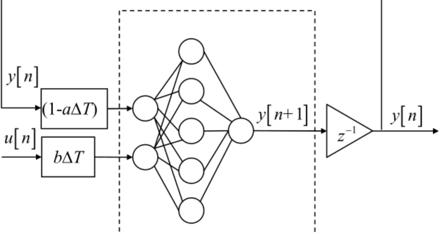
(32) order difference equation, the fitness will be the same. Whether any other weight matrices will lead to larger fitness is a question. It can be said that the GS is better than the fist order difference equation if fitness of the GS is larger with the same sampling time. There remains a second question: how much does the sampling time affect the fitness of the GS. It is known that the fitness will increase as the sampling time decrease in the fist order difference equation, so to reduce the sampling time is necessary. Thus, the question about whether the sampling time has the same influence on the GS with fist order difference equation is taken up in the next chapter.. 3.2.3 Structure with Sampling Time Since the GS is a discrete time system without coefficients related to sampling time, it learns under the fixed sampling time of the training data. As a result, the GS is only suitable for the fixed sampling time, which restricts the use of the GS. One problem is raised: Does any neural network structure exist for arbitrary sampling times after learning, just like the first order difference equation suitable for a first order LTI system? To solve the problem, a structure with sampling time, called ‘SST’ in short, is designed to adapt a wide range of sampling times, as shown in Fig. 3.3, which adopts the parameters of the first order difference equation and is described as ⎡(1 − a ∆ T ) y[n]⎤ y[n+ 1] = W (2 )W (1 ) ⎢ ⎥ ⎣ (b ∆ T )u[n] ⎦. (3.16). where the gains of the inputs is the main difference with the GS. By setting the weight matrices as ⎡1 ⎢1 ⎢ W (1) = ⎢1 ⎢ ⎢1 ⎢⎣1. 1⎤ 1⎥⎥ 1⎥ and W (2 ) = [0.2 0.2 0.2 0.2 0.2] , ⎥ 1⎥ 1⎥⎦ 21. (3.17).

(33) the SST obtains the output same as the first order difference equation. In this case, the SST is available for a wide range of sampling times and subject to an error due to the use of the sampling time. To further increase the fitness, it is required to find different weight matrices based on the evolution strategies, which will be introduced in the next section.. y [ n] (1-a∆T) u [ n]. y [ n+1]. z. −1. y [ n]. b∆T. Figure 3.3 the SST for first order LTI system In this section, except the structure for the fist order difference equation, two types of the structures of the neural network are designed to learn the first order LTI system, and the most difference between these two types is how the sampling time effects. Before simulations, the learning algorithm of these structures will be introduced in the next section.. 3.3 Evolution Strategies In neural network theory, it is an important issue to find the neural network whose weights lead to the global minimum of an error function. Unfortunately, it is difficult to know the minimum is global or not, even for systems without uncertainties. Therefore, instead of global minimum, investigators often develop evolution strategies to search the optimal minimum of fitness function with largest fitness locally, not globally. The backpropagation learning algorithm adjusts the synaptic weights using chain rule 22.

(34) depending on the gradient descent method as (2.6) and (2.7), so the synaptic weights could not be updated using the backpropagation learning algorithm while the inverse dynamic system is unknown. However, the evolution strategies we proposed adjust weights using evolution, but the chain rule according to the fitness function, so it avoid the disadvantage of the backpropagation learning algorithm. It can be said that that the neural network can learn easily using the evolution strategies even if the inverse dynamic system is unknown. According to the origin of species by Darwin [22], individuals less suited to the environment are less likely to survive and to reproduce. Under the limit of the environment, much of the species reproduce sexually, which leads no two individuals are identical generally, and thus the individuals more suited to the environment are more likely to keep their inheritable characteristics to future generations. That is so called nature selection, the most widely used by biologists to represent the scientific model of how species evolve. Here, evolution strategies, depending on nature selection, are proposed for the learning algorithm of the neural network. In the evolution strategies, the given problem is viewed as the environment and every set of weight matrices is viewed as an individual [23]. Basically, the biological reproduction is divided into two groups: sexual and asexual. Individual is different with their parents by sexual reproduction, but it is just identical copy of its parents by asexual reproduction except for mutation. Different with the nature world where the mutation happens with the reproduction unpredictably, it does not happen in the evolution strategies. In general, the species do not reproduce sexually and asexually at the same time, even if hydras and earthworms which can reproduce either sexually or asexually. In the evolution strategies, the reproduction happen both sexually and asexually at the same time. Four points is helpful in sketch out the evolution strategies: the initial individuals creation, the reproduction process, the learning process, and the elite process. Since the generation inherits from the last generation, the initial individuals affect the future offspring; 23.

(35) it means that not arbitrary initial individual after learning will behave as the objective system. By various reproduction processes and the learning processes, the individuals of every generation will be different even if the initial individuals are the same. Further, the elite process chooses the individuals which are more suitable to the problem. In the thesis, the evolution leads to a lot of results depending on its initial population, reproduction process, learning process, and elite process, and any above terms probably fails to learn. These four influences will be discussed next.. 3.3.1 Initial Individuals Creation From (3.13), the structures both contain two weight matrices W(1) aad W(2). In the evolution strategies, the matrices are combined as an individual Wkg , defined as. [. Wkg = w11(1). w12(1). (1) w21. (1) w22. (1) w31. (1) w32. (1) w41. (1) w42. (1) w51. (1) w52. w11(2 ). w12(2 ). w13(2 ). w14(2 ). w15(2 ). ]. (3.18) which is the kth individual of the gth generation. Let g=0, 1, 2,…, and k=1, 2, 3,…, ng where ng is the population size of the gth generation. First, it is known that the initial individuals Wk0 affect the offspring Wkg where g ≠ 0 and not arbitrary Wk0 lead a successful learning. No exact way can decide how these initial individuals are before the evolution. The learning is expected to success even if the initial individuals are given randomly. Unfortunately, it is difficult because of the issue of the local optimal. Note that (3.15) and (3.17) could be thought as good individual of GS and SST, respectively. If the parameters are used to be an initial individual, the probability of success increases. Chapter 4 will show the influences of the initial individuals.. 24.

(36) 3.3.2 Reproduction Process The reproduction process is used for increasing the searching space of the individuals. For the human beings, the offspring combines the half chromosomes of each parent when the sexual reproduction happens. The child contains the half genes from the mother and the other half genes from the father. Not all the reproduction processes of the living things are same to the human begin, such as hydras whose offspring can be produced asexually. Therefore, how to create the offspring is concerned. In the evolution strategies, the individuals Wkg are called the parents and Ωkg are called the children after the reproduction process. In the beginning of the reproduction process, n0 initial individuals have been created using method of Section 3.3.1. Of course, there are many approaches to create children and they can be produced from not only two parents. In the thesis, the reproduction process is divided into two methods: inward method and outward method. The inward method satisfied by Ωkg − Wcg ≤ max Wkg − Wcg. (3.19). k. is introduced first where Wcg expressed as Wcg =. (. 1 W1g + W2g + L + Wngg g n. ). (3.20). is the center of the parents . For example, a child can be created as. (. ). ⎧1 Wngg + W1g , ⎪ ⎪2 Ωkg = ⎨ ⎪1 W g + W g , k +1 ⎪⎩ 2 k. (. ). if k = n g. , otherwise. 25. (3.21).

(37) shown as Fig. 3.4(a), or be created as Ωkg =. (. ). 1 W1g + W2g + L + Wngg , g n. (3.22). shown as Fig. 3.4(b). Besides, the outward method could be used. The children can be created outward as. ( (. ) ). ⎧⎪ Ωkg − Wngg = l W1g − Wngg , ⎨ g ⎪⎩ Ωk − Wkg = l Wkg+1 − Wkg ,. ( (. ) ). if k = n g otherwise. ⎧⎪l W1g − Wngg + Wngg , g ⇒ Ωk = ⎨ ⎪⎩l Wkg+1 − Wkg + Wkg ,. if k = n g. ,. (3.23). otherwise. shown in Fig. 3.5(a), or. (. Ωkg − Wcg = l Wkg − Wcg. (. ). ). (3.24). ⇒ Ωkg = l Wkg − Wcg + Wcg. where l is larger than one, shown in Fig. 3.5(b). In (3.23) and (3.24), the multiple of the distance l affects the children, thus it affects the probability of finding an individual which contains the best optimal value, called the best individual. However, it is unknown what the best individual is, and the effect degree could not be predicted because the evolution strategies not only use the reproduction process. Since the effect of l is unknown, a variable l seems a better choice than the fixed.. (a). (b). Figure 3.4 Illustration of finding children inward 26.

(38) (a). (b). Figure 3.5 Illustration of finding children outward It is mentioned that the variable multiple l can increase the probability of finding the best individual, and be given 0.95 of l in the last generation while the variation of fitness is not more than 5 generations in the evolution strategies. However, when l decreases to smaller than 1, the method is inward, not outward. In this case, a random reproduction process is adopted to replace the original outward process described as (3.24). The new children are reproduced randomly with larger distance than the maximum distance max Wkg − Wcg , shown k. as Fig. 3.6. The purpose of this replacement is to increase the possibility of finding the best individual.. d. center. parent. child. Figure 3.6 Random children creation. 27.

(39) 3.3.3 Learning Process After the reproduction process, there are (2n+1) children when there are n parents. In the learning process, every child learns independently, and the learning process will be introduced in this section. The objective of the learning process is to find an individual whose fitness approaches the optimal value, called optimal individual. Traditionally, the backpropagation learning algorithm uses the gradient of the error function to reach the objective. In the evolution strategies, it doesn’t use the gradient method to decide how the synaptic weights alter. Every step of the learning process tries to find a new individual whose fitness is larger than last step until the process reaches one of the stop conditions. The learning process starts with randomly creating a small enough difference δ Ωtmp (1) around the first individual Ωkg (1) and then obtain the temporal individual Ωtmp (2) = Ωkg (1) + δ Ωtmp (1) .. (3.25). If Ωtmp (2 ) does not lead to an fitness larger than Ωkg (1) , give it up and further find a new temporal individual. Once the fitness created by Ωtmp (2 ) is larger than Ωkg (1) , choose. δ Ωtmp (1) and Ωtmp (2) as the desired difference and individual, that is, δ Ω (1) = δ Ωtmp (1) , and Ωkg (2) = Ωtmp (2) . After the difference δ Ω (1) is determined, the desired individual is updated as the procedure depicted in Fig. 3.7 and described as Ωtmp (s + 1) = Ωkg (s ) + δ Ωtmp (s ). (3.26). 28.

(40) where. δ Ωtmp (s ) = a δ Ω (s − 1) + b δ Ω ⊥ (s − 1). (3.27). b = 1 − a2. and δ Ω ⊥ (s − 1) is the perpendicular vector of δ Ω (s ) and a is chosen randomly between 0 and 1 to avoid the direction of δ Ωtmp (s ) is opposite to δ Ω (s − 1) .. Figure 3.7 finding temporal individual of the next step To find a perpendicular vectors, for example, one method is to choose two entries indexed i and j in the original vector, which is described as. [. v = v1. v 2 L vi L v j. L vn. ]. (3.28). ]. (3.29). and obtain the perpendicular vector as. [. v⊥ = 0 0 L vj. L − vi L 0 .. Although there are other simple ways to find perpendicular vectors, a more complex way which contains more variety is used in the thesis. The origin vector is described as (3.28), and every entry of the perpendicular vector is given randomly first except the index i, determined as v ⊥ = [r1. r2 L ri −1. c ri +1 L rn ]. (3.30). 29.

(41) where c is given as c=−. v1r1 + v2 r2 + L + vi −1ri −1 + vi +1ri +1 + L + v n rn vi. (3.31). such that v ⋅ v ⊥ = 0 . Since the perpendicular vector is decided, δ Ωtmp (s ) could be calculated. The temporal individual of (s+1)th step is determined as (3.26). If Ωtmp (s + 1) leads larger fitness than Ωkg (s ) , keep δ Ω (s ) as δ Ωtmp (s ) and let Ωkg (s + 1) be equal to Ωtmp (s + 1) , otherwise, choose a randomly and find a new perpendicular vector to create a new. δ Ωtmp (s ) again. Then, use the same way to get individual of every step until the learning process reaches the stop conditions. If the fitness of the final step does not reach the desired fitness, suppose it as the optimal fitness and labeled as Ωk,gopt . Every child uses the learning process to find its own optimal fitness. The most common used stop condition is to check whether the fitness reach the desired fitness or not. Besides, the number of the steps could be restricted by experience or the learning could be stopped when the fitness has unchanged for several steps. In the thesis, the stop conditions of the learning process are checking whether the fitness is smaller than the desired and the weights have unchanged for several steps. If the learning process reaches any of the stop conditions, it stops.. 3.3.4 Elite Process It is known that the environment limits the population size of the species, so the number of individuals is restricted no matter the individuals belongs to which generation. Since the meaning of this restriction is to control the population size within limits, the generation length,. 30.

(42) the population size of every generation, or the population size of all generations could be chosen as a restriction. For simplicity, the generation length and the population size of every generation are set to be the restriction. Unfortunately, the restriction of the generation length may stop the learning before learning well, and the restriction of the population size may increase the learning time. To be accurate, the restriction of population size of every generation is the first choice of the evolution strategies and the generation length is set to be very large. It deserves to be mentioned that there are (2n+1) children with their own optimal minimum after the learning process if there are n parents. It tells the number of the individuals is larger than the last generation. Generation by generation, the number of the individuals will become very large and that will increase the learning computation time seriously. Therefore, the population size of every generation should be restricted. The elite process is introduced to solve the problem by choosing some child to be the parent of the next generation. It is an issue which individuals should be kept for the next generation. They can be chosen randomly from the (2n+1) children, but, in this thesis, they are chosen depending on their own optimal fitness. To find n individuals for the next generation, the children are sorted by their fitness. Then, the first n children which contain the largest fitness will be kept. In other words, it is expressed as Wkg +1 = Ωk,gopt. (3.32). where Ωk,gopt contains the kth largest fitness.. According to the above methods, the evolution strategies start from creating n initial individuals. Then do the reproduction process to produce the (2n+1) children. For the (2n+1). 31.

(43) children, use the learning process to find their own optimal fitness. At this time, the elite process is used to reduce the number of the individual to n, and it keeps the number of the individuals unchanged generation by generation. The reproduction process, the learning process and the elite process repeats again and again until the largest fitness reach the desired goal or is unchanged for several generations. The flow chart of the evolution strategies is shown in the next section.. 32.

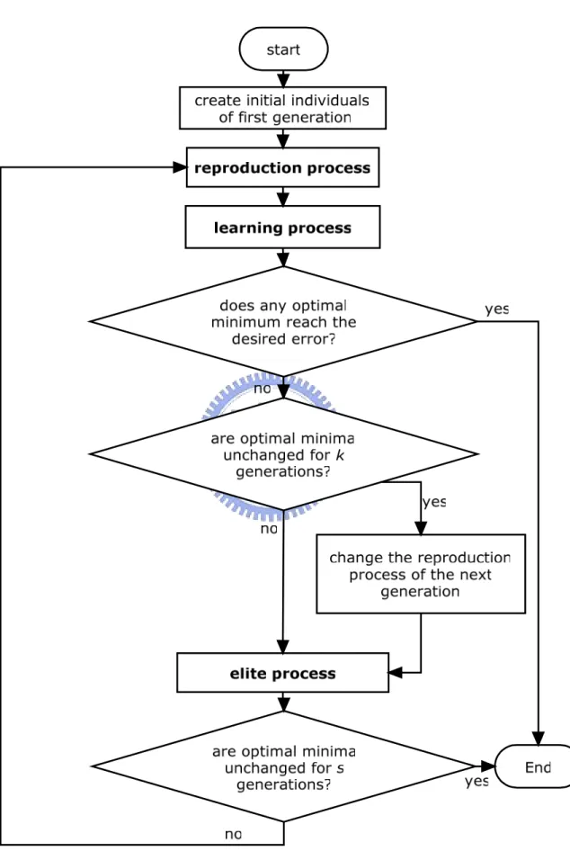
(44) 3.3.5 Flow Chart. Figure 3.8 the flow chart of the evolution strategies 33.

(45) Chapter 4 Simulation Results. In this chapter, the objective system of the neural network is a first order LTI system, described as y& (t ) + y (t ) = u (t ). (4.1). for simplicity. According to the system, the training data are captured with given sampling times when the input function is a step function whose amplitude is equal to 1 and the system initial condition are idled. The fitness function is defined as the negative sum of the errors between the outputs of the first order LTI system and the NN system. The learning procedure indicated in the last chapter was implemented by a Matlab program. In last chapter, it is mentioned that there are some settings which will affect the performance of the evolution strategies, such as the initial individuals and sampling times. Here, the influence of these settings will be discussed, and then the learned neural network using the evolution strategies will be implemented as a controller. The influence of the sampling times will be discussed in Section 4.1, the influence of the initial individuals creation will be discussed in Section 4.2, and then Section 4.3 will show the results of the neural network trained as a controller.. 34.

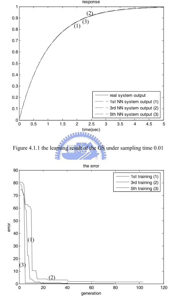
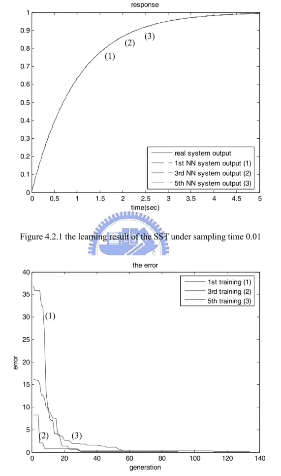
(46) 4.1. Influence of The Sampling Time The influence resolves itself into the following two points: one is the influence of the. sampling time to learning result; the other is the abilities of two neural network structures to adapt different sampling times. The first point will be discussed in the following paragraph. In the first order difference equation, it showed that the fitness increases as the sampling time decreases. It is concerned whether the fitness of the two neural network structures increase as the sampling time decrease like the first order difference equation. There remains a second question about whether the sampling time affects the success rate of the learning result or not. Here, the GS and SST are trained under the sampling time 0.01 and 0.001. Fig. 4.1.1 shows the learning result of the GS when the training data are under sampling time 0.01 at 1st, 3rd, and 5th time. Fig 4.1.2 shows the variation of negative fitness, sum of the error, during the learning process of the GS when the training data are under sampling time 0.01 at 1st, 3rd, and 5th time. Similarly, the objective of Fig. 4.2.1 and Fig 4.2.2 is the SST under the sampling time 0.01, the objective of Fig. 4.3.1 and Fig 4.3.2 is the GS under the sampling time 0.001, and the objective of Fig. 4.4.1 and Fig 4.4.2 is the SST under the sampling time 0.001. Table 4.1 presents the learning results whose initial individual are all given randomly. We define the learning as success learning while the average of the error is smaller than 0.05, and show the result in the Table 4.2.1 and Table 4.2.2. Every case is learned by starting with three different initial random individuals.. 35.

(47) response 1 0.9. (1). 0.8. (2) (3). 0.7 0.6 0.5 0.4 0.3 real system output 1st NN system output (1) 3rd NN system output (2) 5th NN system output (3). 0.2 0.1 0. 0. 0.5. 1. 1.5. 2. 2.5 time(sec). 3. 3.5. 4. 4.5. 5. Figure 4.1.1 the learning result of the GS under sampling time 0.01 the error. 90. 1st training (1) 3rd training (2) 5th training (3). 80 70. error. 60 50 40. (1) 30 20. (3) 10. (2) 0. 0. 20. 40. 60 generation. 80. 100. 120. Figure 4.1.2 the change of the sum of the error of the GS under sampling time 0.01. 36.

(48) response 1 0.9. (3). (2). 0.8. (1). 0.7 0.6 0.5 0.4 0.3 real system output 1st NN system output (1) 3rd NN system output (2) 5th NN system output (3). 0.2 0.1 0. 0. 0.5. 1. 1.5. 2. 2.5 time(sec). 3. 3.5. 4. 4.5. 5. Figure 4.2.1 the learning result of the SST under sampling time 0.01 the error. 40. 1st training (1) 3rd training (2) 5th training (3). 35. (1). 30. error. 25 20 15 10 5 0. (2) 0. (3) 20. 40. 60 80 generation. 100. 120. 140. Figure 4.2.2 the change of the sum of the error of the SST under sampling time 0.01 37.

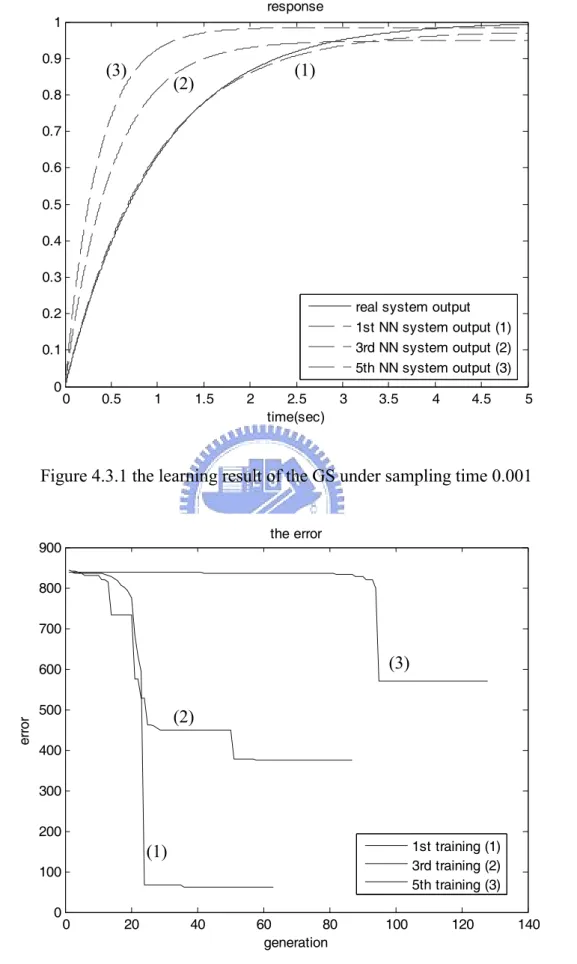
(49) response 1 0.9. (3). (1). (2). 0.8 0.7 0.6 0.5 0.4 0.3. real system output 1st NN system output (1) 3rd NN system output (2) 5th NN system output (3). 0.2 0.1 0. 0. 0.5. 1. 1.5. 2. 2.5 time(sec). 3. 3.5. 4. 4.5. 5. Figure 4.3.1 the learning result of the GS under sampling time 0.001 the error. 900 800 700. (3). error. 600 500. (2). 400 300 200. 1st training (1) 3rd training (2) 5th training (3). (1) 100 0. 0. 20. 40. 60 80 generation. 100. 120. 140. Figure 4.3.2 the change of the sum of the error of the GS under sampling time 0.001 38.

(50) response 1.4. 1.2. 1. (2). (3). 0.8. (1). 0.6. 0.4 real system output 1st NN system output (1) 3rd NN system output (2) 5th NN system output (3). 0.2. 0. 0. 0.5. 1. 1.5. 2. 2.5 time(sec). 3. 3.5. 4. 4.5. 5. Figure 4.4.1 the learning result of the SST under sampling time 0.001 the error. 800. 1st training (1) 3rd training (2) 5th training (3). 700 600. error. 500 400 300. (1). 200 100 0. (2). (3) 0. 10. 20. 30. 40 generation. 50. 60. 70. 80. Figure 4.4.2 the change of the sum of the error of the SST under sampling time 0.001 39.

(51) Table 4.1 the results of learning with different sampling times ∆T = 0.01 generation length. GS. SST. 1st. 78. 89. 2nd. 36. 3rd. ∆T = 0.001. learning time. GS. generation length. SST. learning time. GS. SST. GS. SST. 01:34:55 00:08:13. 62. 47. 01:21:54 00:33:07. 88. 00:50:07 00:09:01. 485. 27. 15:27:51 00:16:57. 102. 66. 01:50:32 00:09:27. 86. 76. 01:12:17 00:55:54. 4th. 81. 38. 01:32:53 00:12:34. 94. 53. 01:43:28 00:39:49. 5th. 54. 133. 01:34:51 00:07:21. 127. 34. 04:42:18 00:28:33. average. 70. 83. 01:28:40 00:09:19. 171. 47. 04:53:34 00:24:52. Table 4.2.1 the error and the accurate rate of learning with sampling time 0.01 ∆T = 0.01 Sum of error. GS. SST. average of error (10-2). GS. SST. Success/Fail. GS. SST. 1st. 0.0740 0.1784 0.01480 0.03568. S. S. 2nd. 0.2939 0.1538 0.05878 0.03076. S. S. 3rd. 1.5743 0.2525 0.31486 0.05050. S. S. 4th. 1.8689 0.4242 0.37378 0.08484. S. S. 5th. 0.1782 0.1291 0.03564 0.02582. S. S. average 0.7979 0.2276 0.15957 0.04552 Success rate(%) 100 100. 40.

(52) Table 4.2.2 the error and the accurate rate of learning with sampling time 0.001 ∆T = 0.001 Sum of error. average of error (10-2). Success/Fail. GS. SST. GS. SST. GS. SST. 1st. 61.3104. 85.9001. 1.22621. 1.71800. S. S. 2nd. 144.4808 118.1299. 2.88962. 2.36260. S. S. 3rd. 374.9141. 4.1978. 7.49828. 0.08396. F. S. 4th. 131.3523. 32.7474. 2.62705. 0.65495. S. S. 5th. 570.8313. 15.3980. 11.41663 0.30550. F. S. average 256.5779. 51.2746. 5.13156. 1.02500 Success rate(%) 60 100. The Fig 4.1.1 and Fig. 4.2.1 show that the learning results are almost the same with the system response when the sampling time is 0.01. Fig. 4.3.1 and Fig. 4.4.1 show that the learning results have some error from the first order LTI system response when the sampling time is 0.001, although the direction of the trend is the same. It means the fitness of the proposed neural network structures increases as the sampling time decrease. Besides, Table 4.1, Table 4.2.1, and Table 4.2.2 tell that the error has no relationship with generation length, and the learning time is independent with the value of the generation length. The Table 4.1 also shows that the learning time increases as the sampling time decrease in the same neural network structure, and the average learning time of the SST is shorter than the GS. Table 4.2.1 and Table 4.2.2 indicate that the larger sampling time produce smaller fitness. It is similar with the first order difference equation. Besides, compared to the success rate, it is clear that the success rate of the GS decreases as the sampling time decreases.. 41.

(53) Since the simulation results show errors are small, i.e. fitness are large, take the best individual with ∆T=0.01 to test the dynamic of the NN system. Here, two significant conditions for a system are variable for validation: the one is the initial condition y(0) of the system, and the other is the input function. Let the initial condition y(0) be 0.5, 2, and -2, and the input function be 2p(t), -2 p(t), and sine function where p(t) is a unit step function. The testing results of the initial conditions are shown in Fig. 4.5.1 to Fig. 4.5.3, and the testing results of the input functions are shown in Fig. 4.6.1 to Fig. 4.6.3. system response 1 0.95. (3). 0.9. (2). 0.85. (1). 0.8 0.75 0.7 0.65. input real system output (1) output of GS (2) output of SST (3). 0.6 0.55 0.5. 0. 0.5. 1. 1.5. 2. 2.5 time(sec). 3. 3.5. 4. 4.5. Figure 4.5.1 testing result when initial condition y(0) is 0.5. 42. 5.

(54) system response 2 input real system output (1) output of GS (2) output of SST (3). 1.9 1.8 1.7 1.6 1.5. (1). 1.4. (2). 1.3. (3). 1.2 1.1 1. 0. 0.5. 1. 1.5. 2. 2.5 time(sec). 3. 3.5. 4. 4.5. 5. Figure 4.5.2 testing result when initial condition y(0) is 2 system response 1. 0.5. (3) (2). 0. (1) -0.5. -1 input real system output (1) output of GS (2) output of SST (3). -1.5. -2. 0. 0.5. 1. 1.5. 2. 2.5 time(sec). 3. 3.5. 4. 4.5. Figure 4.5.3 testing result when initial condition y(0) is -2 43. 5.

(55) system response 2 1.8 1.6 1.4. (3). 1.2. (2). 1. (1). 0.8 0.6 input real system output (1) output of GS (2) output of SST (3). 0.4 0.2 0. 0. 0.5. 1. 1.5. 2. 2.5 time(sec). 3. 3.5. 4. 4.5. 5. Figure 4.6.1 testing result when input function u = 2p(t) system response 0 input real system output (1) output of GS (2) output of SST (3). -0.2 -0.4 -0.6 -0.8 -1. (1). -1.2. (2). -1.4. (3). -1.6 -1.8 -2. 0. 0.5. 1. 1.5. 2. 2.5 time(sec). 3. 3.5. 4. Figure 4.6.2 testing result when input function u = -2p(t) 44. 4.5. 5.

(56) system response 1 0.8 0.6. (1). 0.4. (2). 0.2. (3). 0 -0.2 -0.4. input real system output (1) output of GS (2) output of SST (3). -0.6 -0.8 -1. 0. 0.5. 1. 1.5. 2. 2.5 time(sec). 3. 3.5. 4. 4.5. 5. Figure 4.6.3 testing result when input function u = sin(2t) Fig 4.5.1 to Fig 4.6.3 indicate the neural networks using evolution strategies don't just learn as a specific curve, but the input-output relationship of the objective system. In another words, the learned neural network system behaves similar with the first order LTI system no matter what the initial condition or the input function is. Thus, these results lead to the conclusion that that the neural network using evolution strategies could learn well as a first order LTI system. Since the influence of the sampling time to the fitness does exist, the abilities of two structures to adapt different sampling times must be recalled here. To verify the abilities, take the best learning result under the sampling time 0.01, to test the system under the smaller sampling time 0.005 whose result is shown as Fig. 4.7, and to test under the much smaller sampling time 0.001 whose result is shown as Fig. 4.8.. 45.

(57) system response 1.4. 1.2. 1. (2). (3). 0.8. (1) 0.6. 0.4 input real system output (1) output of GS (2) output of SST (3). 0.2. 0. 0. 0.5. 1. 1.5. 2. 2.5 time(sec). 3. 3.5. 4. 4.5. 5. Figure 4.7 the testing result with ∆ T =0.005 of the learned neural network with ∆ T =0.01 system response 1.4. 1.2. 1. 0.8. 0.6. 0.4 input real system output output of GS output of SST. 0.2. 0. 0. 0.5. 1. 1.5. 2. 2.5 time(sec). 3. 3.5. 4. 4.5. 5. Figure 4.8 the testing result with ∆ T =0.001 of the learned neural network with ∆ T =0.01. 46.

(58) The Fig 4.7 tells that the GS fails, but the SST successes. Fig. 4.7 and Fig. 4.8 indicate that the GS can only be used under a fixed sampling time, but the SST can be used under larger range near the sampling time of the training data. Therefore, the SST is trained with different sampling times, 0.01, 0.001, and 0.0001 using evolution strategies, and then the results will show in Fig. 4.9 and Fig 4.10.1 to Fig. 4.10.3. It demonstrates that the SST can adapt larger rage of the sampling time when it is trained under larger range. It concludes that the SST is better than the GS concerning about the sampling time for learning the first order LTI system. system response 1.4. 1.2. 1. (4) (3). 0.8. (2) (1). 0.6. 0.4. input real system output (1) output of SST: sampling time 0.01 (2) output of SST: sampling time 0.001 (3) output of SST: sampling time 0.0001 (4). 0.2. 0. 0. 0.5. 1. 1.5. 2. 2.5 time(sec). 3. 3.5. 4. 4.5. 5. Figure 4.9 the learning result of the SST with sampling time 0.01, 0.001, 0.0001. 47.

(59) system response 1.4. 1.2. 1. 0.8. 0.6. 0.4 input real system output output of SST: sampling time 0.00001 output of SST: sampling time 0.00005. 0.2. 0. 0. 0.5. 1. 1.5. 2. 2.5 time(sec). 3. 3.5. 4. 4.5. 5. Figure 4.10.1 the testing result under the sampling time smaller than trained sampling time system response 1 0.9. (3). 0.8 0.7. (2). 0.6. (1). 0.5 0.4 0.3 input real system output (1) output of SST: sampling time 0.0005 (2) output of SST: sampling time 0.005 (3). 0.2 0.1 0. 0. 0.5. 1. 1.5. 2. 2.5 time(sec). 3. 3.5. 4. 4.5. 5. Figure 4.10.2 the testing result under the sampling time between trained sampling time 48.

(60) system response 1 0.9 0.8 0.7 0.6 0.5 0.4 0.3 input real system output output of SST: sampling time 0.05 output of SST: sampling time 0.5. 0.2 0.1 0. 0. 0.5. 1. 1.5. 2. 2.5 time(sec). 3. 3.5. 4. 4.5. 5. Figure 4.10.3 the testing result under the sampling time larger than trained sampling time. 4.2. Influence of The Initial Weights Setting. In the last section, it is said that the success rate decreases and the learning time increases as the sampling time decreases. How to let the error reach the global minimum is an important issue for neural network investigators because it is easy to consider the local minimum as the global minimum. Thus, the local minimum may the main reason for failure learning. However, it is worthy noticing that the first order difference equation provides a set of adequate parameters to approach the first order LTI system. In the following, one of the initial individual is given depending on the parameters of the first order difference equation and compare with the random initial individual. The general structure using the initial individual given by the first order difference equation is called GSi. Since the SST has used the parameters of the first order difference equation in the network, SST is not discussed in this 49.

(61) section. The learning objective is the first order LTI system with sampling time 0.001, and one of the initial individual is given by the first order difference equation with sampling time 0.01. The learning result is shown in Figure 4.11.1 to Fig. 4.11.2, and Table 4.3. Table 4.3 learning results of GS with sampling time 0.001 GS with ∆T = 0.001 generation length. learning time. sum of error. average of error (10-2). success/fail. 1st. 70. 03:02:29. 3.9376. 0.07875. S. 2nd. 49. 02:40:50. 25.6901. 0.51380. S. 3rd. 850. 06:34:49. 1.1476. 0.02295. S. 4th. 235. 14:45:59. 22.7393. 0.45479. S. 5th. 117. 05:01:20. 93.8409. 1.87682. S. average. 264. 06:25:05. 29.4711. 0.58942. 50. success rate (%). 100.

(62) response 1.4. 1.2. (3). 1. (1). 0.8. (2). 0.6. 0.4 real system output 1st NN system output (1) 3rd NN system output (2) 5th NN system output (3). 0.2. 0. 0. 0.5. 1. 1.5. 2. 2.5 time(sec). 3. 3.5. 4. 4.5. 5. Figure 4.11.1 the learning result of the GS under sampling time 0.001 the error. 800. 1st training (1) 3rd training (2) 5th training (3). 700 600. error. 500 400 300. (1). 200. (3). 100. (2) 0. 0. 100. 200. 300. 400 500 generation. 600. 700. 800. 900. Figure 4.11.2 the change of the sum of the error of the SST under sampling time 0.001 51.

(63) Compared with the Table 4.1 to Table 4.2.2, Table 4.3 indicates that the success rate of GSi is larger than GS. It is worthy noticing that the sum of error of 3rd learning is smaller than the first order difference equation, 2.0302. It means the GS could perform better than the first order difference equation under the sampling time 0.001. However, the average of the learning time is larger than the last section. It reminds that the learning time is independent of the success rate. Similar to Section 4.1, two significant conditions for a system are also variable for validation: the one is the initial condition of the system, and the other is the input function. The influences of these two conditions are shown in Fig. 4.12.1 to Fig. 4.13.3 using the 3rd learning result. Thus, as the figures indicate, no matter what the initial condition and the input functions are, the learned neural network behaves corresponding to the first order LTI system. system response 1 0.95 0.9. (1) (2). 0.85 0.8 0.75 0.7 0.65 0.6. input real system output (1) output of GS (2). 0.55 0.5. 0. 0.5. 1. 1.5. 2. 2.5 time(sec). 3. 3.5. 4. 4.5. Figure 4.12.1 testing result when initial condition y(0) is 0.5. 52. 5.

(64) system response 2 input real system output (1) output of GS (2). 1.9 1.8 1.7 1.6 1.5 1.4 1.3 1.2. (1) (2). 1.1 1. 0. 0.5. 1. 1.5. 2. 2.5 time(sec). 3. 3.5. 4. 4.5. 5. Figure 4.12.2 testing result when initial condition y(0) is 2 system response 1. 0.5. (1) (2). 0. -0.5. -1. -1.5. -2. input real system output (1) output of GS (2) 0. 0.5. 1. 1.5. 2. 2.5 time(sec). 3. 3.5. 4. 4.5. Figure 4.12.3 testing result when initial condition y(0) is -2 53. 5.

(65) system response 2 1.8 1.6. (1) (2). 1.4 1.2 1 0.8 0.6 0.4. input real system output (1) output of GS (2). 0.2 0. 0. 0.5. 1. 1.5. 2. 2.5 time(sec). 3. 3.5. 4. 4.5. 5. Figure 4.13.1 testing result when input function u = 2p(t) system response 0 input real system output (1) output of GS (2). -0.2 -0.4 -0.6 -0.8 -1 -1.2 -1.4. (1) (2). -1.6 -1.8 -2. 0. 0.5. 1. 1.5. 2. 2.5 time(sec). 3. 3.5. 4. 4.5. Figure 4.13.2 testing result when input function u = -2p(t) 54. 5.

(66) system response. 1 0.8 0.6 0.4 0.2. (1) (2). 0 -0.2 -0.4 -0.6. input real system output (1) output of GS (2). -0.8 -1. 0. 0.5. 1. 1.5. 2. 2.5 time(sec). 3. 3.5. 4. 4.5. 5. Figure 4.13.3 testing result when input function u = sin(2t). 4.3. Implement as a Controller. According to the results of the last two sections, it concludes that GS and SST using the evolution strategies have good performance on learning a first order LTI system. Further, implement it as a first order LTI controller to control the given plant to verify its ability. Here, a first order and a second order LTI system are the objective plant of the learned controller. Section 4.3.1 use the first order LTI plant to test the learned neural network structures, and Section 4.3.2 use the second order LTI plant to test.. 55.