多世代產品的創新擴散概念模型

(1)

國立交通大學

經營管理研究所

碩士論文

多世代產品的創新擴散概念模型

A Conceptual Innovation Diffusion Model of

Multi-Generations Products

研究生：張碩文

指導教授：唐瓔璋教授

(2)

多世代產品的創新擴散概念模型

A Conceptual Innovation Diffusion Model of

Multi-Generations Products

研究生：張碩文 Student：Shuo-Wen Chang 指導教授：唐瓔璋 Advisor：Ying-Chan Tang 國立交通大學經營管理研究所碩士論文 A Thesis

Submitted to Institute of Business and Management College of Management

National Chiao Tung University in Partial Fulfillment of the Requirements

for the Degree of

Master of Business Administration

January 2010

Taipei, Taiwan, Republic of China 中華民國九十九年一月

(3)

I

多世代產品的創新擴散概念模型

學生：張碩文指導教授：唐瓔璋

國立交通大學經營管理研究所碩士班

摘要

1969 年的 Bass model 將消費者劃分為創新者和模仿者，成功的捕捉到新產品在市場上的擴散行為；Bass 更指出只要擁有連續三期以上的銷售資料，Bass model 就能估計新產品的尖峰銷售量及其發生的時間。Norton 和 Bass 更在 1987 年針對當時的高科技產品發展多世代產品的擴散模型(Substitution Bass Model)，企圖模擬新舊世代產品間的擴散關係及替代關係。然而，過去所定義的新產品是指市場上從未見過的創新應用，例如第一台電視、第一部電腦、第一支手機..等等。但在現代的時空環境背景之下，市場上鮮少有真正符合定義的新產品，取而代之的是所謂的「次世代產品」。因此，本研究的貢獻之一，即是以Bass model 的創新擴散為基礎，建立新的模型以捕捉次世代產品佔有舊世代市場的行為，並預測舊世代產品的尖峰銷售量及其發生的時間。此外，本文也說明過去Bass Model 的預測曲線擁有極高準確

度的原因。另一方面，本文融合Bass Model 的預測方法、Tellis 的起飛點 (1997)

以及本文的新模型，建立一套方法幫助經理人預測新舊世代產品在未來不同時間的銷售量。

本研究指出了新舊科技間的替代行為，而未來的研究也可應用本文的架構，進而探討不同品牌間的關係，將新產品領域更進一步拓展。

(4)

II

A Conceptual Innovation Diffusion Model of

Multi-Generations Products

Student：Shuo-Wen Chang Advisors：Dr. Edwin-Tang

Institute of Business Management

National Chiao Tung University

ABSTRACT

Bass model captured the diffusion behavior of new products in the market successfully in 1969 by dividing consumers into innovators and imitators. Bass indicated that Bass model can estimate sales peak and the timing of sales peak if they get the sales data during three continuing periods. In 1987, Norton and Bass

developed a multi-generations model (Substitution Bass Model) to simulate the diffusion behavior and substitution behavior among multi-generations.

However, what they defined new products are those innovative applications which never exist in the market, such as the first TV、the first computer、the first cell phone. Nowadays, there are rarely real new products but new generations. Consequently, one of our contributions is creating a new model based on Bass model, capturing the behavior that how new generations occupy old markets and predicting sales peak and the timing of it of old generation. In addition, this article explains the reason of the high accuracy of Bass model. On the other hand, this article merges the estimating method of Bass model, Tellis’s takeoff (1997) and our new model, constructing a way for managers to forecast the sales amount of generations in the future.

This article indicates the substitution behavior among generations. Future research can also apply our framework to discuss the relationship between different brands, expanding the new product field.

(5)

III

Acknowledgement

比起其他人的兩年研究所生涯，我的「三年半」幾乎是其他同學的一倍!雖然時間稍長了一點，但這段過程卻是十分的精彩絕倫；大學從理工科畢業的我，對商科幾乎沒有半點底子，但憑藉著經管所教授的深厚功力和自己的興趣、熱情，歷經了三年多的磨練之後，現在竟也能對於各種商業行為有著自己的見解，也能針對企業的五管領域進行研究分析，這一切都要感謝經管所的各個教授!尤其是帶領我一窺行銷奧秘的唐瓔璋教授，老師讓我建立了一套屬於自己的思考邏輯，並用世界上各領域的行銷案例培養我們的行銷觀念，這一切的過程對我這個極想創業的學生而言十分重要也十分珍貴! 除此之外，我很感謝一路相陪的經管所夥伴；從剛進來接了招生說明會一直到後來接所學會幹部，謝謝翊瑋、小花、念青、盈芊和宜凡一直不厭其煩的幫忙處理所上事務，也謝謝每次活動都很挺我們的憲哥、小美，讓我覺得活動辦得很有意義。也謝謝球隊的夥伴們，雖然兩年內我們都沒有晉級，但我們用平均不到 175 的身高、不到 75 的體重硬是贏下了幾場比賽，這也是很好的回憶了! 另外也要謝謝一起參加各個行銷競賽的夥伴，念青、小兔、煜均、阿白…等，憑著大家的努力合作，每個行銷競賽我們都闖進了複賽；雖然最終都沒能拿下大獎項，不過能進到全國前幾十名的複賽名單，我也覺得很滿足了；這也告訴我們要繼續努力，人外有人，天外有天! 最後要感謝我的阿 Po，讓我在寫論文的階段可以很專心的投入，不被打擾 XD 張碩文謹誌中華民國九十九年一月二十二日

(6)

IV

List of Figures

Figure 1 Different type of adopters categorized by Rogers ... 10 Figure 2 Five stages of the adoption process ... 11 Figure 3 S‐curve ... 12 Figure 4 Bass’s categorization of adopters ... 13 Figure 5 Takeoff, Slowdown and product life cycle ... 16 Figure 6 Sales Data of DRAM ... 26 Figure 7 Parabola ... 28 Figure 8 Sum of Generations ... 29 Figure 9 Constitutions of Generations ... 31 Figure 10 Assess sales amount ... 35 Figure 11 Components of S2 ... 36

(9)

1

Chapter 1 Introduction

1.1 Research Background and Motives

During 20th century, plenty of new products have emerged in the world. What we named “new products” is that they solve human problems by unexpected new

technologies. Humans need time to learn new products and get used to them. In other words, humans have to change their behavior from a familiar one to a new one. In the past two decades, human living are transforming immensely as the continuing

progress of technology. Different necessaries which are based on information, Internet, digitization and communication technology appeared around human surroundings such as MP3 player, cell phone and notebook. Recently, the prevailing iPod even becomes a new lifestyle. Besides, the innovative Tivo breaks the limitation that we have to follow the TV schedule to wait for what we want to see. We can choose programs we like any time. Tivo helps people arrange their leisure time conveniently. Thus, to past consumer, accompanying the pace of digitization and the improving technology, there emerged unimaginable new products which can change human living custom. In this article, we discuss not only new products but innovations.

An innovation is an idea, practice, or object perceived as new by an individual or other unit of adoption (Rogers, 1962). In Tellis’s opinion, innovation, the process of bringing new products and services to market, is one of the most important issues in business research (Tellis, 2006). And if an adoption of an innovation by an individual or other unit of an adoption can diffuse quickly, we call the innovation is success. So far, there is a great deal of articles researching all aspects of diffusion of innovations

(10)

2 within forty years.

However, nowadays, these kinds of innovating applications are getting mature, there are few breakthroughs invented in the global market. What we have is the “Next Generation”. Engineers are devoting to develop new products which are based on old products to pursue growth. For example, wireless communication is advancing from 2G to 3G to wimax and operating system is progressing from Windows XP to Vista. That is to say, there are nearly no genuine “new products” today. Therefore, the main purpose of this article is trying to contribute to develop a model to discuss the

relationship between “New generations” and the old ones because that the

competition and replacement relationship are more important in the future. On the other hand, not every innovation can be adopted successfully by consumer. Although the information we received is almost how an innovation succeeded, how fast a product diffused, the truth is that there were large number of products failed or cannot be popularized by the masses behind the successful ones, such as the failure of the UltimateTV of Microsoft. Consequently, one of the purposes of this article is to discuss the diffusion relationship among those products which substitute each other. These kinds of products include its own multiple generations, meaning that 3G can capture the market of 2G, and opponent’s products. The importance of researching diffusion relationship is that corporations usually invest a lot on new technologies and new products. In order to make a precise decision to avoid wasting money on

launching new products, production and inventory, estimating the growth of new generation and the decline of old generation accurately becomes a crucial issue to managers.

(11)

3

The same as previous articles, this article narrows the rage of the definition of new products to consumer durables. The feature of consumer durables is that consumer won’t repurchase within short time and purchase one unit at a time. Under this condition, we can analyze the diffusion behavior of targeted products. In regard to previous knowledge, we’ll discuss particularly in the review.

The theory of adoption and diffusion of new ideas and new products by a social system has been discussed at length by Rogers (Bass, 1969). Early 1960,

understanding how a new product succeed became a popular issue. Rogers, a master of communication studies, first published the book “diffusion of innovations＂, explaining why some good ideas and products are able to become popular and spread quickly while the others can’t. The writing has been affecting many fields widely, including marketing, economics, anthropology, sociology and so on, especially in communications and technology adoption studies. As the publishing of diffusion of innovations, there sprang up a lot of articles exploiting the concept to research the issue of new products in the new product area of marketing.

During the development of knowledge on new products within the forty years, the main directions on which new product area focus can be categorized into five groups：

1.1.1 Methods of enhancing new product development processes

The papers here consider that firms face a challenge in deploying the “voice of the customer” in the R&D, engineering and manufacturing stages of product development. The articles deal with how a firm uses what customer eager to proceeds innovation.

(12)

4

The advantage lies not only on rising revenue but increasing the probability of adoption. Griffin and Hauser (1993) focused on identifying, structuring, and

prioritizing customers needs, illustrating how a product-development team might use the voice of the customer to create a successful new product. In addition to answering how to identify customers’ needs, they illustrated how customers’ needs cbe arrayed into a hierarchy of primary, secondary, and tertiary needs, so that ultimately

customers＇ preferences can be measured and compared. This article only discusses how an organization coordinates efficiently.

Shocker and Srinivasan (1979) highlighted the emergence of a new, proactive research model – multi attribute research – which investigates the structure of customer decisions with respect to the market offerings of a firm and its competitors. In order to predict customer behavior in a wide range of future environments, they focus on developing an understanding of customer decision, so that they can forecast customers＇ move even in the absence of data.

More recently, Nowlis and Simonson (1996) investigated the factors that moderate the impact of a new feature on brand choice. They proposed two principles: multi attribute diminishing sensitivity and performance uncertainty. They demonstrated that how new features affect market share and sales volume depends on the preexisting characteristics of the products to which those new features are added.

The accomplishment of this field lies on forwarding diffusion of new products by designing new product features accurately. Nonetheless, this field cannot assist companies to manage the growth and decline of their launched multiple generation

(13)

5 products.

1.1.2 Preproduction testing and evaluation of new product designs

Pretest is an important procedure to observe the reactions of customers. It can decide whether a new product is launched or which part need to be adjusted. This field investigates how a new product be evaluated and tested before the investment for production is made. Here includes research on beta testing procedures, pretest market models, prelaunch forecasting methods, information acceleration, and test market methods.

Silk and Urban (1978) introduced ASSESSOR which is a set of measurement procedures and models. It is able to estimate the sales potential of a new packaged good before test marketing, thereby assisting companies to save the costs from the high failure rate of new packaged goods in test markets. Afterward Urban and Katz (1983) published a validation of the ASSESSOR model. Their results suggested that the ASSESSOR pretest market system did well in predicting test market shares. Recently, Urban, Weinberg, and Hauser (1996) showed how to forecast consumer reaction to a real new product. Their approach made use of a multimedia

virtual-buying environment that simulated future situations and experiences, making it possible to determine whether the new product would be viable at target launch date.

This area is able to help the decision of launching a new product or not. However, it is useless to help manage a launched product.

(14)

6

1.1.3 Methods of forecasting the adoption and growth of new products

Bass (1969) proposed a masterpiece which has been influencing new product field tremendously, named Bass model. Bass model allows us for calculating the sales peak and the timing of the sales peak by data from earlier stage. It can also help depict the successive increases in the number of adopters and predict the continued diffusion process. Bass model improved our understanding of the structural, estimation, and conceptual assumptions underlying diffusion models of new product adoption. Many researches cited Bass model and used it to develop revised models which are added other important variables like price and advertisement. Mahajan, Muller, and Bass (1990) provided a detailed review which categorized new product research into five areas: basic diffusion models, coefficient estimation considerations, flexible diffusion models, refinements and extensions, and use of diffusion models. They identified a number of research issues within these five areas that could be help make more effective, realistic and practical diffusion models

Robertson and Gatignon (1986) pointed out that previous researches only focused on individual level rather than on organizational level. They therefore presented an alternative paradigm based on organizational adoption and competitive behavior instead of individual adoption.

Norton and Bass (1987) further proposed an improved model to solve the multiple generation issue on high-technology products. The launch of new generations of high-technology products will capture the market of earlier generations, including its own earlier types and its competitors. Besides, multiple generation products became

(15)

7

important due to the common situation that new technologies were applied in old applications instead of creating a new application, resulting in new generations

competed with old generations rather than finding a new market. Thus, managers have to consider the impact of the launch of a new generation particularly to calculate the accurate purchases of earlier generations and the new generation and to avoid destructive competition on the growth of its earlier generations. The model that Norton and Bass developed includes diffusion effect and substitution effect, based on Bass diffusion model (1969). Norton and Bass also demonstrated the forecasting properties of their model.

By the end of the 1980s, there existed abundant conceptual diffusion researches which surveyed different coefficients, providing enough data for meta-analysis. Sultan, Farley, and Lehmann (1990) made empirical generalizations from a

meta-analysis of more than 200 sets of coefficients. Their results suggested that the diffusion process is affected more by such factors like word of mouth than by innate innovativeness of consumers. Furthermore, they also indicated that the coefficient of innovation is fairly stable under a wide variety of conditions but the coefficient of imitation varies widely with the innovation type, the estimation procedure, and the presence of other coefficients.

More recently, Golder and Tellis (1997) proposed the existence of takeoff point which is characterized by a dramatic increase in sales, advancing our understanding of the growth of innovation. They investigated the data of “really new＂ household consumer durables and found that the takeoff tends to appear as an elbow-shaped discontinuity in the sales curve. Consequently, they further addressed the essential

(16)

8

issues that how much time does a new product need to reach the takeoff. Their work gave managers an understanding which can help observe whether a new product diffuses successfully or not.

1.1.4 Market entry and defense strategies

Hauser, Tellis, and Griffin (2006) reviewed researches on innovation and classified these researches into five fields. They spend two fields on reviewing market entry strategies, which included technological revolution, strategies for entry, and portfolio management, and reviewing defending against market entry strategies, which

included the rewards of entrants and strategies of defense. The research stream here addressed whether, when, and how a firm should innovate or should defend against innovation by competitors.

Ofek and Sarvary (2003) suggested that R&D competence can encourage a leader to invest in order to obtain technology leadership, while the presence of reputation effects can encourage a leader to reduce the investment on R&D, resulting in alternating leadership between a duopoly of firms.

A number of early papers supported the statement that entering a market first will have long-term advantages. On the other hand, Golder and Tellis (1993) used different methodology to reexamine the rewards to pioneers and argued that even if there is a pioneering advantage, later entrants are often able to conquer it. Shankar, Carpenter, and Krishnamurthi (1998) also showed that an innovative late mover can grow faster than the pioneer, slow the pioneer’s diffusion and reduce the effectiveness

(17)

9

of the pioneer’s marketing spending. Besides, innovative late movers are advantaged in that their diffusion can hurt the sales of other brands, but their sales are not affected by competitors’ diffusion. In contrast, non-innovative late movers have smaller potential markets, lower repeat rates, and less marketing effectiveness than a pioneer.

1.1.5 Contextual and structural drivers of innovation

Chandy and Tellis (2000) examined whether new entrants are more likely to introduce

radical innovation. They found that prior to World War Ⅱ, small firms and new entrants were more likely to introduce radical innovations. However, the pattern reversed after the war.

1.2 Research Objective

After reviewing previous five fields in new product area, some theories are still useful in present society while others are too simple to describe the complex competition of today’s multiple generations. Hence, this article aims to create a multiple generation model based on Original Bass Model (1969) and Substitution Bass Model (1987) in order to solve the competition relationship among multiple generation products.

(18)

10

Chapter 2 Literature Review

2.1 Diffusion of Innovation

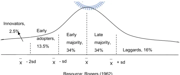
Rogers published the first edition of diffusion of innovation at 1962 and published the fourth edition at 1995. Rogers defined innovations as the processes by which that innovation “is communicated through certain channels over time among the members of a social system.” He categorized adopters of any new innovation into five groups: innovators (2.5%), early adopters (13.5%), early majority (34%), late majority (34%) and laggards (16%) by using two statistical coefficients, mean and standard deviation. Figure 1 illustrates the categorization. And each person can belong to different

categories for different innovations.

This classification and the five terms have been accepted and used for many years by researchers. Rogers also indicated the four factors of diffusion of innovations: time, innovation, communication channels and social system. He re-categorized the five stages of adoption in the later editions as figure 2.

Resource: Rogers (1962) - sd

X ¯

Figure 1 Different type of adopters categorized by Rogers

X ¯ Laggards, 16% Late majority, 34% Early majority, 34% Early adopters, 13.5% Innovators, 2.5% + sd X ¯ - 2sd X ¯

(19)

11

(1) Knowledge: the individual is first exposed to an innovation but lacks information about the innovation. (2) Persuasion: the individual is interested in the innovation and actively seeks information/detail about the innovation. (3) Decision: the individual takes the concept of the innovation and weighs the advantages and disadvantages of using the innovation and decides whether to adopt or reject the innovation. (4)

Implementation: the individual employs the innovation to a varying degree depending on the situation. During this stage the individual determines the usefulness of the innovation and may search for further information about it. (5) Confirmation: the individual finalizes their decision to continue using the innovation and may use the innovation to its fullest potential. (Rogers, 1995)

2.1.1 S-curve

Rogers also indicated the presence of S-curve which is the graph formed by cumulative adoptions. Figure 3 is an example of S-curve, showing a cumulative number of adopters over time.

Figure 2 Five stages of the adoption process

Knowledge Persuasion Decision Implementation

Confirmation Reject

Accept

(20)

12

Diffusion of Innovation in a certain social system follows s-shaped distribution. According to diffusion theory, a diffusion process of innovation in a social system is capable of self-sustaining when the adopters reach a certain ratio of the total

population of a system. This ratio, sometimes replaced by absolute numbers of adopters, is critical mass. Usually, the critical mass is about 10%~20% of the total population of a system (Rogers, 1995; Ure, 2001；Valente, 1995). After reaching the critical mass, the diffusion process of an innovation will take-off, which means spreading drastically. This process continues until most of the potential adopters have adopted the innovation. Finally, the process levels down and reaches the saturated point which is the point that no increases happens on new adopters. This process, as a result, forms s-shaped curve.

2.2 Bass Model

However, in spite of the particular discussion of the book” diffusion of innovation”,

Numb er s New adopters Cumulative number of adopters Time Figure 3 S-curve Resource：Rogers (1962)

(21)

13

Bass (1969) considered that the discussion is largely literary and not supported by real data. Consequently, Bass proposed a model to capture the tendency of the diffusion process by real data.

Bass used the data of consumer durables to analysis the diffusion behavior because of the characteristic that consumer durables are not repurchased in a short time and usually are purchased one unit at a given time. This characteristic help Bass observe the pure diffusion behavior without misleading by repurchases. Bass applied the concept of hazard function to new product growth model, assuming that the

probability that an initial purchase will be made at T given that no purchase has yet been made is a linear function of the number of previous buyers. Bass expected to find the sales peak of consumer durables and the timing of sales peak based on present data. According to Bass’s definition, the function is:

Where P(T) is the probability that an initial purchase will be made at T given that no purchases has yet been made and Y(T) is the cumulative adopters. The coefficients p, q and m will be explained next. Bass redefined Rogers’s categorization of adopters (innovators, early adopters, early majority, late majority and laggards) into two classifications:

(1)

Early adopters

Innovators Early majority Late majority Laggards

Innovators Imitators

Figure 4 Bass’s categorization of adopters

(22)

14

(1) Innovators: adopt an innovation independently of the decisions of other individuals in a social system

(2) Imitatorss : are influenced in the timing of adoption by the decisions of other members in the social system

Due to Bass’s categorization, the constant p in equation1 represents the effect of innovators in a social system, standing for the probability of an initial purchase at T(0). When T=0, meaning that at initial stage, the cumulative purchases of an

innovation are supposed to be zero ( Y(T)=0 ). Consequently, the adopted probability

at T(0) should be p, . The term shows how imitators react.

Imitators always adopt an innovation as others do. The more adoption people made, the more pressure imitators get. Therefore, as cumulative purchases Y(T) raise, the adopted probability P(T) goes up. The constant q is used as the coefficient of imitators and the constant m represents the total potential market of initial purchases in product life cycle. According to Bass’s definition that P(T) is the probability that an initial purchase will be made at T given that no purchases has yet been made, P(T) can also expressed by following:

Where f(T) is the likelihood of purchase at a given time T and

Thus, F(T) times total potential purchases m equal to cumulative adopters Y(T) and f(T) times m equal to S(T), which is defined as the sales happened at a given time T. Besides, the integration of S(T) is the cumulative adopters Y(T).

(23)

15 and

Expanding equation2 and replacing by F(T), equation2 becomes

Solving this nonlinear differential equation4 can help draw the curve of f(T) and F(T) by giving T and find the sales peak and the timing of sales peak.

In order to get coefficient p, q, m, Bass replaced f(T) by and F(T) by ,

turning equation 4 into following:

This equation shows the behavioral rationale that initial purchases made by both innovators and imitators and innovators are not influenced by the number of adopters while imitators “learns” from others. Thus p is related to innovation and q is related to imitation. Then, Bass connected the concept of bell-curve that the sales at a given time form a bell-shaped curve as time goes on with equation5. That is to say, Bass used real data of an innovation to create the bell curve function: Since (3) (4) (5) (6)

(24)

16

Furthermore, due to b = q – p, Bass obtain this quation .

Rearranging the above equation, it will be .

Thus, .

After calculating coefficient p,q,m, the sales peak and the timing of the sales peak can be found easily.

2.3 Takeoff

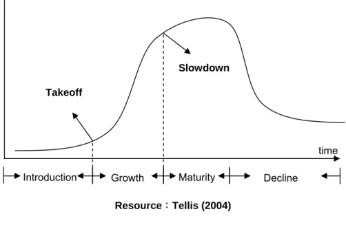
Golder and Tellis (2004) refered to takeoff and slowdown of product life cycle. We summarize it and the stages of product life cycle in figure 5 :

Takeoff is the timing where introduction stage turns into growth stage and

Slowdown Maturity Growth Introduction time sales Decline Takeoff

Figure 5 Takeoff, Slowdown and product life cycle

(25)

17

slowdown is the timing where growth stage turns into maturity stage. Next, we’ll review literatures following the sequence of these stages above.

Bass model presumed that there existed a certain purchases (p times m) at initial stage. However, sales of most successful new products are very low at introduction stage and soared suddenly at a certain time which is called “takeoff”. Then sales are grown fast after the point takeoff.

Gort and Klepper (1982) defined the diffusion of innovation as the spread in the number of producers engaged in manufacturing a new product. Nonetheless, we can’t assure if the increase of producers is identical with the increase of consumer adoption because that they did not observe the real consumer behavior. Kohli, Lehmann and Pae (1999) defined an “incubation time” as the time between product development and market launch, finding that the duration of incubation time will affect the coefficient of Bass model. The longer the incubation time existed, the lower the coefficient of innovation (p) and the longer the time to sales peak happened.

Golder and Tellis (1997) defined the point “takeoff” of new product sales as the time that the introduction stage turns into growth stage of product life cycle. They found that the takeoff tends to appear as an elbow-shaped discontinuity in the sales curve showing an average sales increase of over 400%. They also indicated that when the base level of sales is small, a relatively large percentage increase could occur without signaling the takeoff. In contrast, when the base level of sales is large, the takeoff sometimes occurs with a relatively small percentage increase in sales. In the end, they examined several marketing variables and discovered that price and

(26)

18

marketing penetration strongly correlates with takeoff. Tellis, Stremersch and Yin (2003) investigated the takeoff-related issue in Europe and showed that sales of most new products display a distinct takeoff in various European countries and the

time-to-takeoff varies substantially across countries and categories. Their research displayed that cultural difference explains the different duration to takeoff while economic factors can’t.

Since this sudden increase on sales need a lot of resource to cooperate like

production, inventory and logistics, understanding the occurrence of takeoff and what drives it is very crucial to managers. Nevertheless, the present literatures about takeoff were all verified by the data of successful new products rather than all launching product. Those literatures, therefore, can only help measure when the takeoff happens rather than judge whether the takeoff happens or not.

2.4 Growth

Although Bass model has been a great paradigm aiming to deal with growth stage in marketing field, there still existed some limitations had to be break. Following are extensions of Bass model and limitations of Bass model.

2.4.1 Redefinition of Bass model

In contrast to Bass’s explanation of coefficients p, q that p is related to innovator and q is related to imitator, Rogers’s definition that innovators are the first 2.5% adopters of all potential adopters is quite different from Bass’. In other words, Bass

(27)

19

defined innovators as buyers who are not influenced by others instead of buyers who adopt an innovation first. So how does Bass model associate with classic normal distribution proposed by Rogers?

Mahajan, Muller and Srivastava (1990) proposed a rewritten form of Bass’s basic assumption (equation2).

Where n(t) is equal to s(t) and N(t) is equal to Y(t) in Bass model.

They suggested that the term “innovator” in Bass model should not be called innovator because those buyers are necessarily not the first adopters in Rogers’s definition. Therefore, they cited Lekvall and Wahlbin’s opinion (1973) that the coefficients p, q in Bass model should be referred to as the coefficient of external influence and the coefficient of internal influence, respectively. They thought that the potential adopters of an innovation are influenced by two means of communication: mass media (external influence) and word of mouth (internal influence). And innovators are influenced only by mass media communication while imitators are influenced only by word of mouth communication.

Lekvall and Wahlbin also proposed an explicit expression to estimate the total adopters affected by external influence.

Consequently, adopters influenced by internal influence are

This explanation helped connect Bass model with Rogers’s work. Next, how does Bass model compare with Rogers’s five categories? This answer is simple. Mahajan,

(7)

(28)

20

Muller and Srivastava (1990) indicated that the point of inflection represents one standard deviation away from the mean of the normal distribution. Thus, finding the point of inflection of Bass’s equation can yield five categories of Bass model.

2.4.2 Limitation of lacking data

Bass model yields good prediction when adding sales data. However, managers want to know how consumers react to new products before launching instead of after launching. To solve this problem, Mahajan, Muller and Bass (1990) suggested that if no data are available, parameter estimates can be obtained by using either

management judgments or the diffusion history of analogous products.

2.4.3 Including Marketing Variables

Bass model do not contain marketing variables such as price and advertisement. Managers would like to know how to improve sales through those variables. Kamakura and Balasubramanian (1988) discovered that the decline of price only influences the adopted probability of products which have higher price.

Price seems to play different role among products. Horsky and Simon (1983) added the expenditure of advertisement of producers at given time T into Bass model. Bass, Krishnan and Jain (1994) created the Generalized Bass model, adding two factors, price and advertisement, into Bass model:

Where x(t) is present marketing investment, the expression is as following: (9)

(29)

21

is the change of price while is the change of expenditure on advertisement. They found that the fitness of Bass model is good enough as the percentage of change on decision variables remains constant while the fitness provided by Generalized Bass model is better than by Bass model as the percentage of change on decision variables alters remarkably.

2.4.4 Including Supply Restrictions

Some researchers discussed other restrictions in management. Jain, Mahajan, and Muller (1991) discussed supply side limitation such as limited production ability and limited logistics ability. They deemed that consumers transform into waiting applicants from potential adopters first, then transform into adopters in the end. Here is their model:

And

The term reflects the change of waiting applicants. This change consists of

increases on waiting applicants A(t) and the number of adopters N(t) and decreases because waiting applicants A(t) becomes adopters. c(t) is the supply coefficient, meaning that a certain percentage of waiting applicants can really get the merchandise due to limitation on supply side. They produced the formula of increasing new

adopters as following:

(30)

22

Ho, Savin and Terwiesch (2002) further discussed the real situation: In the presence of a supply constraint, potential customers who are not able to obtain the new product join the waiting queue, generating backorders and potentially reversing their adoption decision, resulting in lost sales.

2.4.5 Including Competitive Effects

Some researchers considered the influence on the diffusion of present brands resulted from the entry of new competitors. One new brand may result in two effects: (1) A new brand will increase the market potential of the product category due to product diversity and raising promotion. (2) A new brand will reduce the diffusion of present brands due to competition. Mahajan, Sharma and Buzzell (1993) investigated camera market, indicating that the new brand entry, Kodak, got exceeding 30% sales of existing brand Polaroid’s potential buyers while bringing about the market

expansion. Krishnan, Bass and Kumar (2000) investigated cell phone market, finding that the diffusion effect created by new brands entry differs among different markets. Some increase market potential while others obstruct the diffusion speed of their competitive brands. Although these articles discussed competitive impact, they didn’t explain the impetus behind the phenomenon.

2.4.6 Including Technological Generations

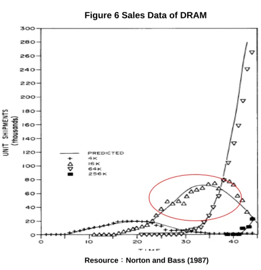
Norton and Bass (1987) assessed the market penetration of successful high-tech multi-generations products based on Bass model. They used 4k, 16k, 64k ,256k DRAM as samples, developing a model to deal with the substitution effect among

(31)

23

multi-generation products. To facilitate our later discussion, we use the term “Substitute Bass model” to represent their model. Following lists a formula of a simple situation between two generations:

τ2 is the launching time of second generation, Yi(t) is the cumulative sales at given

time T of generation i, Ｆi(t) is the cumulative adopted rate and mi is market potential

of generation i. This model captured the diffusion and substitution effect quite well. Next, Norton and Bass (1992) continually applied this substitution model to other industry such as recording media and computer products and pharmaceuticals. Mahajan and Muller (1996) explained a leapfrogging phenomenon: some consumer skip a generation, adopting the latest generation directly. Kim, Chang and Shocker (2000) tried to coordinate substitution effect and complementary effect in a new model.

(32)

24

Chapter 3 Research Methodology

3.1 The drawback of Substitution Bass Model

In Substitution Bass model, each generation has the same coefficient of external influence p, coefficient of internal influence q and has its own potential market (m1,

m2...mn). This assumption generated the same cumulative density function F of each

generation, which means generations have the same growth pattern if they don’t influence each other. The only difference among those cumulative density function is the emerging time. Then Bass identified these nonlinear equations:

Yi (t) = shipments of generation i, (where a is q/p and b is p + q),

mi = the incremental potential served by the ith generation, that is, that not capable of

being served by any generation j < i.

τ

i is the emerging time of generation i.

There is a crucial concept behind this model. It assumed that there exists two markets m1 and m2. m1 consists of the consumers who are attracted by the functions

of generation 1 while m2 are attracted by the new functions of generation 2. In

addition, most new generations own the functions of old generations. Thus, m1 may

change their mind to buy generation 2 but m2 has no possibility to buy generation 1

(33)

25

Since m1 and m2 are different market segments, the life style and the consumer

behavior of m1 and m2 may exists inconsistency. Some market segments are

influenced easily by words of mouth while the others are affected quickly by mass media.

Thus, the coefficients of external and internal influence of different generations should be different (p1≠p2≠….. pn and q1≠q2≠……qn) Our first step is to relax the

assumption of the Substitution Bass model that the coefficients of internal influence, q1, q2…qn and external influence p1, p2…pn are the same.

Returning to the Substitution Bass Model, we realize that parts of potential sales of the previous generation transfer to the next generation. For example, parts of potential market m1 switch to the sales of generation 2. Then sales S2 consist of its expanding

application and the transition from m1. Bass solved substitution behavior of

successive generations by giving all generations a certain cumulative function F, isolating each generation’s potential market, generating transferring equations and using data to observe the fitness between real data and estimated curves.

Consequently, the different shapes of curve are caused by its own potential market and the transfer of previous potential market. However, following our relaxation of the equal coefficients of external and internal influence, it should be generate two different cumulative functions F1 and F2.

Next, we try to prove F1 F2 …. Fn. As we can see in this graph derived from Bass’

(34)

26

Although its R2 values of those three curves are remarkably high (S1 (t): 0.9672, S2

(t): 0.9646, S3 (t): 0.9993), we can easily observe that the gap between real sales and

estimated sales becomes bigger when the next generation takes off. The forecast of generation i is inaccurate when generation i + n (n =1,2,3..etc) started to grow or have started growing. The forecast is only accurate in the preceding periods. Therefore, we may say that the high R2 values result from the preceding periods.

Besides, the Substitution Bass model aims to deal with the high-technology product. Nevertheless, the data it used is the unit shipments of different DRAM and SRAM. Today, most high-technology products we mentioned are consuming electronic

Resource：Norton and Bass (1987)

(35)

27

products. The tendency of consuming electronic products is very different from those elements which are inserted into them. The quantity of those elements is not equal to the real sales of consuming electronic products. As we know, in consuming electronic products, suppliers accept new generations and eliminate old ones to force consumer to buy a new generation. Thus, the tendencies of adopting different generations of DRAM and SRAM are more alike. In other words, using the data of DRAM and SRAM instead of the data of the sales of consumer electronic products is not a suitable method to handle this high-technology issue. The data of DRAM and SRAM cannot stand for the real sales of consumer and the timing of consumer’s adoption. To sum up, we think the high R2 values is caused by the data during preceding periods and by the data from inserted elements instead of the real sales of consuming

electronic products. According to previous discussion, generations influence each other. The method of calculating the coefficients of Substitution Bass model can only capture the sales tendency when generation i is not influenced by the following generations but fails to yield a good prediction to generation i when generation i+1 has started to grow.

We should focus on the phenomenon: When next generation starts to grow or has been started growing, the prediction will have a bigger deviation. Because

Substitution Bass model already captures the transitional behavior, we can easily presume that the inaccuracy is resulted from the unprecise emerging F. This

presumption fits with our relaxation that the same coefficients of external and internal influence of different generations are wrong. Different coefficients must result in different cumulative density function F. The identical cumulative density function F produced by Substitution Bass model, of course, will generate inaccurate

(36)

28 forecasting curve.

3.2 Research Framework

3.2.1 Parabola

To develop our equation, we have to explain our basic principle. Given two downward parabolas Y1 and Y2,

,

We can generate a new equation that:

From equation13, the combination Y remains a parabola as the following graph.

Besides, observing the following graph (figure 8) derived from Substitution Bass (13) Y Y Y2 Y1 X Figure 7 Parabola

(37)

29

model, we plus all the sales together and find that the curve of the sum seems to match with a certain parabola. This finding fits with the principle of equation 13. In diffusion behavioral aspect, the sum of all generations represents a diffusion process of a certain category so that the curve of the sum will match with a certain parabola. Therefore, in our model, we don’t separate each generation from others but combine them, using a systematic point of view to solve this issue. We think the forecast of the diffusion of whole market sales is more accurate than individual product sales.

On the other hand, equation 13 can help explain why the R2 of Bass’s evaluation are so high ( Norton, John A ; Bass, Frank M 1987, 1992).

Bass (1969) succeeded in using bell-curve to simulate the sales at a given time S(t).

Thus, in multi-generation environment, no matter the transition of sales occur or Figure 8 Sum of Generation

(38)

30

not, the sum of the sales of all generations at a given time T must forms a parabola. This explains why Bass always succeeded in good fitness because Bass investigated the whole market of a certain category. In our model, we’ll start from the whole market sales and try to assess the interaction among brands.

3.2.2 Conceptual Diffusion Model of Multi-Generations Products

Initial purchase or replacement purchase

Following that, we need to define all the purchases more clearly. In reality, most people buy old generation first and purchase a new generation few years (even few months) later. However, we can’t take this kind of behavior as “replacement

purchases” because they pursue a new one for stronger entertainment or for satisfying themselves. In other words, they won’t buy if the new one is similar with the old one. Therefore, we should still take this kind of purchases as what Bass defined, “initial purchase”. Since we take it as initial purchase, we can still follow Bass’ basic

accepted assumption, “the probability that an initial purchase will be made at T given that no purchase has yet been made is a linear function of the number of previous

buyers”. That is, , is a linear function of the number of previous buyers.

Unlike Substitution Bass model, we doubt that the transition behavior equation shouldn’t be written like equation 12.

(39)

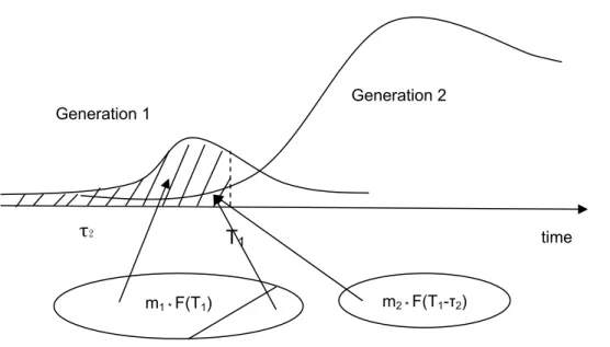
31 As we can see in figure 9,

When t = T1, parts of m1 times F(T1) people adopt generation 1 and the rest switch

to generation 2 while m2 times F(T2) people adopt generation 2 if there is no advanced

generation. Our argument about the Substitution Bass model lies on that m1 has no

impact from generation 2 before τ2. But according to their

equation , it seems that they presume all m1 is affected

by generation 2 at the given time t= T1. Thus, we set up a variable α(t) to represent the

transitional fraction of old generation and construct our model:

Where is the cumulative adopters of generation i, is the potential market of generation i, is the launching time of generation 2 and is the cumulative density function of generation i. Following our previous discussion, we relax the limitation of the same F, allowing different generation has different F.

(14) Figure 9 Constitutions of Generations

T1 Generation 1 time Generation 2 m1 * F(T1) m2 * F(T1-τ2) τ2

(40)

32

captures the transition behavior while equation 14 owns adoption and transition behavior.

Next, we add the concept of substitution model proposed by Fisher and Pry (1971). Their result is that the log of the ratio of the market share of the succeeding

technology to that of the first is a linear function of time:

; j > i

Where ai and aj are the fractional market shares of innovations at time t, j is newer

than i. k is a constant of proportionality, i and j are technologies. Equation 15 can be related to our transition fraction because what Fisher and Pry discussed is how new technology replace old one in original market. We can generate following equation from equation 15:

Since and has the same total market m = , we can rewrite equation 16:

;

From equation 17, we know and we can use present data to calculate the constant k. Then, according to , we construct the following equation:

Differentiating equation 14 and applying to equation 18:

(15)

(16)

(17)

(18)

(41)

33

To solve this linear first-order differential equation, we have to calculate the integration factor I(t) first:

Thus, following the solution that :

To solve the right complicated integration function, we have to apply numerical quadrature rules by matlab to calculate the real value of it. If we get the value of right item, can be measured due to the predictable . The calculation method will be discussed in next chapter. What we focus on here is the sales peak and the timing of sales peak. Since the value of has helped for predicting the future state of generations, it’s unnecessary to find .

Following is how to find the sales peak of S1(t) and the timing of it.

( Si(t) is the sales purchased at a given time t, )

Since , we, therefore, can calculate the value of S1(t) easily

by adding the predictable exogenous values S(t) and the exogenous constant k. Then we can draw the forecasting curve of S1(t).

Because equation 20 is a function of time, we are able to differentiate it:

(20) (20)

(42)

34

Given the formula consisted of coefficients p, q, m from Bass model,

We replace equation 21 by above formulas:

In order to find the timing of sales peak, we must set equation 22 equal to zero. And we note that the exponential value and coefficients of p, q, m must exceed zero.

Consequently, only at the time that or , the sales of

generation 1 per unit time reach its sales maximum or minimum amount. In next chapter, we’ll discuss which time is the timing of sales peak of generation 1.

(21)

(43)

35

Chapter 4 Discussion

4.1 Assessing sales amount

Following is the operating procedure of generating sales prediction.

When t = T1, there is only generation 1 existing in the market. By applying sales

data of generation 1, managers can easily predict by applying Bass’s method. This forecast is accurate because no sales of generation 1 switch to generation 2. However, the forecast appears deviation since generation 2 has launched. According to our previous discussion, we abandon the isolating data from generation 1 and generation 2 because the individual data from both generations actually affected by two potential adopters.

Therefore, combining both data to generate an aggregate data is a precise way to find . The finding of aggregate sales S(t) doesn’t directly help managers because what managers care is the sales and the future market position of their products. But by applying equation 20, we can produce the forecasting sales

τ

Generation2

Generation1

Figure 10 Assess sales amount

(44)

36

curve of S1(t) ( ) and can, of course, calculate S2(t).

From equation 23, obviously, we can get S1(t) and S2(t) after estimating the

constant k. By applying the sales of generation 1 and generation 2 to equation 18 as Fisher and Pry, a certain constant k is available. Finally, we obtain S1(t) and S2(t)

through the aggregate sales S(t) and the estimated constant k.

4.2 Assessing density function

The same as above method, using the data during the time before the launching time (τ of generation 2, the density function f1 and the cumulative density function F1

can be estimated by the coefficients p1, q1, m1. We emphasize that f1 cannot be used to

generate the accurate amount of sales when other generations appear but can help produce the potential density function f2 of next generation.

The method is simple. From figure 11, sales of generation 2 at a given time compose of switch from S1 and original sales of generation 2 S2. Thus, the gap

Original curve of Generation2 Original S2 Switch from S1 Practical curve of Generation2 Figure 11 Components of S2 (23)

(45)

37

between the practical sales of generation1 and the forecast of generation1 generated by f1 must be the switching part to generation 2.

Where S12(t) is the switching part to generation 2

Since the sales of generation 2 consist of the potential adopters of generation 2 and the switch of generation 1,

Practical data of generation 2 S2(t) minus the switching part S12(t) brings S2original.

By treating S2original as the original sales data of generation 2, we are able to produce

the coefficients of p2, q2, m2 and then the density function f2 can be formed. F2 can

also be found by integrating f2 but the density function f2 is enough for us to calculate

the variable α(t) which represents the transitional fraction of old generation.

4.3 The transitional fraction α(t)

According to equation 20 that , using numerical

quadrature rules through matlab can solve α(t). And if we let the time t be infinity, the ultimate allocation state of both generations can be estimated.

From above equation, managers will know how many adopters of generation 1 change to generation 2 and realize the whole practical markets of both generations they need to serve.

(46)

38

Estimating α(t) at any time is unnecessary because both S1(t) and S2(t) are available

by previous method and temporary cumulative sales Y1(t) and Y2(t) aren’t very

important to managers. However, we can still estimate them:

As the procedure of calculating α(t), both integrations of S1(t) and S2(t) need using

numerical quadrature rules by computer to solve it.

4.4 The timing of sales peak

Generation 1:

By setting equation 22 that

equal to zero, we can find that S1(t) reaches its sales maximum and minimum when

and .

4.4.1 Two extreme values

Comparing t1* and t2*, which is bigger depends on the amount of three coefficients.

If t1* is earlier than t2*, it means t1* is the timing of sales peak and t2* is timing of the

minimum sales. Since S1(t) goes up at early stage and is replaced step by step by

generation2, the presumption that the earlier time t1* is the timing of sales peak is

reasonable. Note that the timing t2* is equal to the timing of sales peak of the whole

market category S(t) (Bass,1969). Thus, the timing of sales minimum of S1(t) is the

(47)

39

generation2 and generation2 probably has a quite large potential adopters. Both conditions make S1(t) reaches its maximum at t1* and minimum at t2*. In contrast, if

t2* is earlier than t1*, it means the timing of sales peak of generation1 is equivalent to

the whole market, standing for that there is rare percentage of S1(t) changes to

generation2 and the potential adopters of generation1 is much bigger than generation2. This situation results in a small constant k and causes a longer time t1*.

4.4.2 Only one extreme value

If k is less than p plus q, we cannot count t1* because of the definition of napierian

logarithm (ln). In other words, the timing of sales peak of generation1 is equal to the whole market. Therefore, like above discussion, there is rare percentage of S1(t)

changes to generation2 and the potential adopters of generation1 is much bigger than generation2.

4.5 Sales peak

Generation 1:

If generation1 reaches its sales peak at T = t1*, we replace t1* with and S(t)

with the coefficients p, q, m into equation 20 that . The sales peak in

terms of the coefficients p, q, m is:

(48)

40

Finally, we know when is the timing of sales peak and the amount of sales peak of generation 1 as long as estimating the aggregate coefficients p, q, m and the constant k. In the end, we have to point that we can obtain two curves S1(t) and S2(t) by

generating coefficient k and aggregate sales curve. Consequently, we are able to find the sales peaks and the timings of sales peaks of both generations easily by observing the curves we produced.

(49)

41

Chapter 5 Conclusion and Suggestion

5.1 Conclusion

In order to forecast sales accurately, managers should understand the knowledge of new product growth. The first step is following Tellis and Golder (1997) that the takeoff tends to appear as an elbow-shaped discontinuity in the sales curve showing an average sales increase of over 400%. That is to say, managers have to observe the soaring sales increase of over 400% before applying sales data to produce sales forecast because Bass model need sales data which are made after takeoff point to generate an accurate prediction.

After crossing the takeoff point, managers who are responsible for the first generation just follow Bass’s method to generate coefficients p, q, m and then calculate the timing of sales peak and the sales amount.

Besides, using potential market m times the density function f1(t) is able to estimate

S1(t). Thus, by giving different times, managers can draw the predicted sales curve.

After new generation reaches the takeoff point, managers start calculating the sum of two generations’ sales and exploiting the aggregate data to generate the aggregate

(50)

42

sales forecast. Since the forecast of the total market is more precise and the interaction between two generations follows the conclusion of Fisher and Pry (1971), managers

are able to estimate the sales tendency by and .

Giving different times t, managers can also draw the sales curves of both generations. In addition, after new generation comes out, the reduction in S1(t) ( )

is switching to generation2. Therefore, using the sales data of gneration2 minus the switching part from generation1 produces the original coefficients p2,q2,m2 and the

density function of generation2. The purpose of getting original information of generation2 is to find the transitional fraction α(t).

By letting the time be infinite ∞ , managers can measure the ultimate distribution of both generations. Knowing the final distribution is very important because

managers can realize how many customers they need to serve and how many assets and facilities they need to invest. Calculating can prevent over-investing.

In the end, managers are able to find the timing of sales peak and the sales amount of generation1 by the coefficients from total sales:

If the timing of sales peak is ,

The sales amount will be

(51)

43

In regard to generation2, since we can draw the sales curve of generation2, it is not difficult to predict when will generation2 reaches its peak. In fact, generation2 are usually influenced by next generation. Thus, differentiating to find the timing without considering the impact from next generation is definitely generating a wrong forecast.

5.2 Limitation and Future research

5.2.1 A lack of data of generation2

In Mahajan and Muller’s review of new product growth (1990), they reveal that managers can apply their experience to guess the value of coefficients p, q, m when there is no data existing. Following their discussion, managers are able to draw the forecast curve without data.

However, there is no truly new product today. What we have is new generation. Therefore, managers get to know the new launching product must be influenced by previous generation. Thus, only founding the average values of coefficients k, p2, q2,

m2 can help managers guess the descending S1(t) and rising S2(t). Furthermore, given

that managers know the average values of coefficients, managers can decide the launching timing of new generation to prevent generation1 from losing too much sales to generation2. Managers should let generation2 substitutes for generation1 after generation1 matures.

(52)

44

5.2.2 Competition between different brands

This article aims to deal with the issue that new technology replace old one. Therefore, parts of potential sales of generation1 change to generation2.

We presume that people won’t go back to adopt old generation. But, if we research the competition behavior between different brands, the situation must be more

complex. People may switch to generation2 from generation1 and switch back to generation1 again. Thus, constituting an improved model based on the concept of this article may solve this issue.

(53)

45

Reference

Griffin, A.; Hauser, J.R.，” The Voice of the Customer”，Marketing Science，Vol. 12, No. 1， pp. 1-27，Winter 1993

Shocker, A.D.; Srinivasan, V.，” Multiattribute Approaches for Product Concept Evaluation and Generation: a Critical Review”，Journal of Marketing Research，Vol. 16，No. 2，pp. 159-180，May 1979

Silk, A.J.; Urban, G.L.，” Pre-Test-Market Evaluation of New Packaged

Goods: A Model and Measurement Methodology”，Journal of Marketing Research， Vol. 15，No. 2， pp. 171-191，May 1978

Ofek, E.; Sarvary, M.，” R&D, Marketing, and the Success of Next-Generation Products”，Marketing Science，Vol. 22，No. 3，pp. 355-370，Summer 2003

Sultan, F.; Farley, J.U.; DR Lehmann，” A Meta-Analysis of Applications of

Diffusion Models”，Journal of Marketing Research，Vol. 27， No. 1，pp. 70-77 ， Feb 1990

Bass, Frank M，” A New Product Growth for Model Consumer Durables”， Management Science (pre-1986)，15, 5，ABI/INFORM Global，Jan 1969

Tellis, G.J.; Stremersch, S.; Yin, E.，” The International Takeoff of New Products: The Role of Economics, Culture, and Country Innovativeness”，Marketing Science，

(54)

46 Vol. 22，No. 2，pp. 188-208，Spring 2003

Urban, G.L.; Weinberg, B.D.; Hauser, J.R.，” Premarket Forecasting of Really-New Products”，The Journal of Marketing，Vol. 60，No. 1，pp. 47-60，Jan 1996

Urban, G.L.; Katz, G.M.，” Pre-test-Market Models: Validation and Managerial Implications”，Journal of Marketing Research，Vol. 20，No. 3，pp. 221-234，Aug 1983

Gatignon, H.; Robertson, T.S.，” Technology Diffusion: An Empirical Test of

Competitive Effects”，The Journal of Marketing，Vol. 53，No. 1，pp. 35-49，Jan 1989

Norton, F.A.; Bass, Frank M，” A Diffusion Theory Model of Adoption and

Substitution for Successive Generations of High-Technology Products”，Management Science，Vol. 33，No. 9，pp. 1069-1086，Sep 1987

Norton, J.A.; Bass, Frank M，” Evolution of Technological Generations: The Law of Capture”，Sloan Management Review，33, 2，ABI/INFORM Global，Winter 1992

Hauser, John; Tellis, G.J.; Griffin, A.，“Research on Innovation: A Review and Agenda for Marketing Science”，Marketing Science，Nov/Dec 2006

Gort, M.; Klepper, S.，” Time Paths in the Diffusion of Product Innovations”，The Economic Journal，Vol. 92，No. 367，pp. 630-653，Sep 1982

Golder, P.N.; Tellis, G.J.，” Pioneer Advantage：Marketing Logic or Marketing Legend ?”， Journal of Marketing Research，Vol. 30，No. 2，pp. 158-170，May 1993

(55)

47

Golder, P.N.; Tellis, G.J.，” Will It Ever Fly? Modeling the Takeoff of Really New Consumer Durables”，Marketing Science，Vol. 16，No. 3，pp. 256-270，1997

Kohli, R.; Lehmann D.R.; Pae, Jae，” Extent and Impact of Incubation Time in New Product Diffusion”，Journal of Product Innovation Management，1999

Chandy, R.K.; Tellis, G.J.， ” The Incumbent's Curse? Incumbency, Size, and Radical Product Innovation”，The Journal of Marketing，Vol. 64，No. 3，pp. 1-17，July 2000

Rogers, E.M.，Diffusion of Innovations，1962

Nowlis, S.M.; Simonson, I，” The Effect of New Product Features on Brand Choice”， Journal of Marketing Research，Vol. 33，No. 1，pp. 36-46，Feb 1996

Ho, T.H.; Savin, S.; Terwiesch, C.，” Managing Demand and Sales Dynamics in New Product Diffusion under Supply Constraint”，Management Science，Vol. 48，No. 2， pp. 187-206，Feb 2002

Krishnan, T.V.; Bass, F.M.; Kumar, V.，” Impact of A Late Entrant on the Diffusion of A New Product/Service”，Journal of Marketing Research，2000

Mahajan, V.; Muller, E.; Bass, F.M.，” New Product Diffusion Models in Marketing: A Review and Directions for Research”，The Journal of Marketing，Vol. 54，No. 1， pp. 1-26，Jan 1990

(56)

48

Mahajan, V.; Muller, E.，” Timing, Diffusion, and Substitution of Successive

Generations of Technological Innovations：The IBM Mainframe Case”，Technological Forecasting and Social Change，1996

Mahajan, V.; Sharma, S.; Buzzell, R.D.，” Assessing the Impact of Competitive Entry on Market Expansion and Incumbent Sales”，The Journal of Marketing，Vol. 57，No. 3，pp. 39-52，July 1993

Shankar, V.; Carpenter, G.S.; Krishnamurthi, L，” Late Mover Advantage： How Innovative Late Entrants Outsell Pioneers”，Journal of Marketing Research，Vol. 35， No. 1，pp. 54-70，Feb 1998