國立交通大學
物理研究所
碩 士 論 文
原子序 1 到 4 的原子基態和氫原子高階諧波產生的計算
Calculation of the Ground State of Atom Z=1-4 and
High-Order Harmonic Generation for Hydrogen Atom
研 究 生:
范力文
指導教授:
江進福 教授
原子序
1 到 4 的原子基態和氫原子高階諧波產生的計算
Calculation of the Ground State of Atom Z=1-4 and High-Order Harmonic
Generation for Hydrogen Atom
研究生: 范力文
Student: Li-Wen Fan
指導教授: 江進福
Advisor: Tsin-Fu Jiang
國 立 交 通 大 學
物 理 研 究 所
碩 士 論 文
A Thesis
Submitted to Institute of Physics
College of Science
National Chiao Tung University
in partial Fulfillment of the Requirements
for the Degree of
Master
in
Physics
July 2014
Hsinchu, Taiwan, Republic of China
中華民國 一零三 年 七 月
i
原子序
1 到 4 的原子基態和氫原子高階諧波產生的計算
國立交通大學 物理研究所 碩士班
摘 要
最近數十年隨著密度泛函理論(density functional theory)和電腦的發展,藉由數值方 法達成原子系統相關性質的準確計算逐漸可行。本研究目標在於對原子系統基態的 Kohn-Sham 計算以及研究透過 Krieger-Li-Iafrate(KLI)程序近似最佳等效位能(optimized effective potential)對自我交互作用修正後的準確性。在基態計算的基礎上,模擬在強場 下的原子系統是另一個目標。廣義擬值譜法(generalized pseudo-spectral method)是對於數
值解Kohn-Sham 方程獲得 Kohn-Sham 軌域以及數值解 Poisson 方程獲得 Hartree 位能的
有效方法。對於時變計算,以分離運算子法(split operator method)處理時間算子。在結果
的部分,我們先從原子序 1 到 4 以不同的交換相關泛函的 Kohn-Sham 計算獲得總能和
其分量,再與前人的結果比較以驗證我們的計算可靠。再進一步,我們用KLI 程序近似
最佳等效位能並執行只有交換泛函的計算,結果顯示總能和游離能在自我交互作用修正 後的準確性。最後,我們模擬在雷射場的氫原子並獲得高階諧波產生頻譜。
ii
Calculation of the Ground State of Atom Z=1-4 and High-Order Harmonic
Generation for Hydrogen Atom
Student: Li-Wen Fan
Advisor: Tsin-Fu Jiang
Institute of Physics
National Chiao Tung University
ABSTRACT
The accurate calculation about properties of many-electron atomic system may be performed by numerical method in recent few decades due to the development of density functional theory and computer. The aim of the present research was to perform Kohn-Sham (KS) calculations in ground state of atomic system and investigate the accuracy of the KS calculations with optimized effective potential (OEP) approximated by Krieger-Li-Iafrate (KLI) procedure to correct the self-interaction. Based on the calculation of ground state, simulating dynamics of atomic system in intense field is the other aim. Generalized pseudo-spectral (GPS) was the useful method to numerically solve KS equation to find KS orbitals and Poisson’s equation to find Hartree potential. For time-dependent calculations, spilt operator method was used to deal with the time operators. In the results section, we first obtained the total energies and their components from the KS calculations for atoms Z=1-4 with various exchange-correlation functionals and compared them with other works to make sure our calculation is reliable. Next, we performed the KS calculations with exchange-only functional and OEP approximated by KLI procedure, and we displayed the accuracy of total energies and ionization energies without self-interaction. Finally, we simulated the dynamics of a hydrogen atom in the laser field and obtained the high-order harmonic generation (HHG) spectra.
iii
誌 謝
感謝江進福教授這兩年多的教導,使我受益良多。此外,特別感謝李
漢傑博士、唐平翰博士、鄧德明博士、鄭世達博士(按姓氏筆劃順序)在
研究過程中給與我各種幫助。最後感謝家人的支持,讓我無後顧之憂,完
成碩士學位。
Contents
Chinese Abstract i English Abstract ii Acknowledgement iii Table of Contents iv List of Tables viList of Figures vii
1 Intorduction 1
2 Methods 3
2.1 Quadratures and Grids . . . 3
2.1.1 Gaussian Quadrature . . . 3
2.1.2 Gaussian Grids and Weights . . . 4
2.1.3 Mapping Funciton . . . 5
2.2 Generalized Pseudo-Spectral Method (GPS) . . . 8
2.2.1 Polynomial Interpolation and Cardinal Functions . . . 8
2.2.2 Cardinal Functions for Orthogonal Polynomials . . . 9
2.2.3 Derivatives of Cardinal Functions . . . 9
2.2.4 Differential Matrix . . . 12
2.3 Application of GPS to Schr¨odinger Equation . . . 16
2.3.1 Radial Equation Represented in x Domain . . . . 16
2.3.2 Construction and Symmetrization of Hamiltonian Matrix . . . 18
2.4 Application of GPS on Poisson’s Equation . . . 24
2.4.1 Separation of Radial Part from Poisson’s Equation . . . 24
2.4.2 Construction of System of Linear Equations . . . 25
2.4.3 Determination of Boundary Conditions . . . 27
2.4.4 Correction to Solver . . . 28
2.4.5 Example: Potential Due to Square of Eigenstate . . . 30
2.5 Split Operator Method . . . 33
2.5.1 Intorduction . . . 33
2.5.2 Extension for Time-Dependent Schr¨odinger Equation . . . 34
2.5.3 Treatment of Hamiltonian Operator . . . 35
2.5.4 Programming Scheme . . . 38
3 Theory 40 3.1 Density Functional Theory (DFT) . . . 40
3.1.1 Kohn-Sham Theorem . . . 41
3.1.2 Exchange and Correlation Functionals . . . 42
3.1.3 Optimized Effective Potential (OEP) . . . 45
3.1.4 Krieger-Li-Iafrate Approximation (KLI) . . . 46
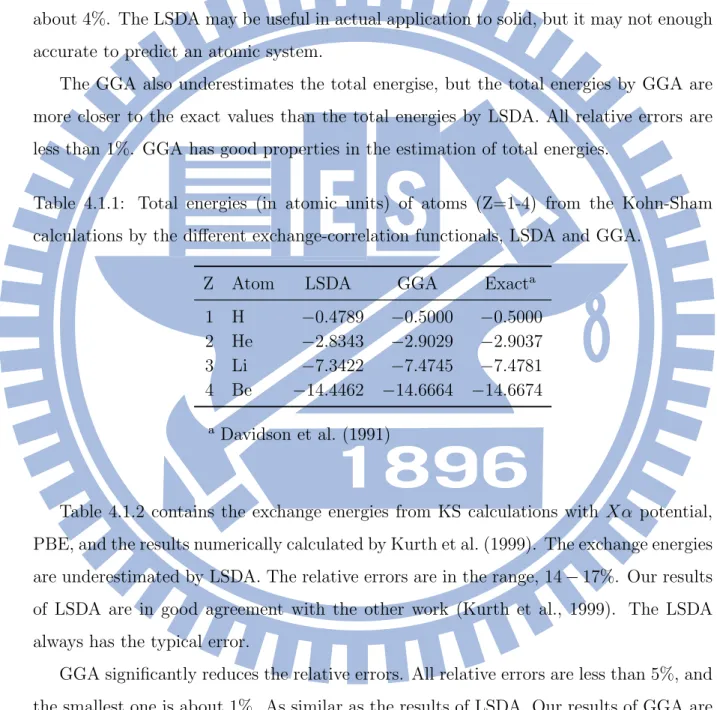
4 Results and Discussion 48 4.1 Kohn-Sham Calculation of Neutral Atom . . . 48
4.1.1 Kohn-Sham Calculation with Various Functionals . . . 48
4.1.2 Kohn-Sham Calculation with OEP Method and KLI Approximation 51 4.2 Hydrogen Atom in Intense Laser Fields . . . 53
4.2.1 High-Order Harmonic Generation (HHG) . . . 53
Bibliography 58
A Legendre Polynomials 62 B Numerical Calculations of Gradient and Laplacian 64
List of Tables
2.2.1 Relative errors of the first derivatives and second derivatives numerically calculated by method 1 and method 2 on 21 GLL grids. . . 14 2.2.2 Relative errors of the first and second derivatives individually evaluated by
method 1 and method 2 at the first point r(x0) = 0 of various numbers of
GLL grid. . . 15 2.3.1 Energy levels of neutral hydrogen atom from the solution of radial equation
with angular quantum numbers, l = 0− 2, by GPS method. . . 22 2.4.1 Relative errors of Hatree potential at the points near the boundaries from
the numerical solution of Poisson’s equation by GPS. . . 31 4.1.1 Total energies (in atomic units) of atoms (Z=1-4) from the Kohn-Sham
calculations by the different exchange-correlation functionals, LSDA and GGA. . . 49 4.1.2 Exchange energies (in atomic units) of atoms (Z=1-4) from the Kohn-Sham
calculations by the different exchange functionals, LSDA and GGA. . . 50 4.1.3 Correlation energies (in atomic units) of atoms (Z=1-4) from the
Kohn-Sham calculations by the different exchange-correlation functionals, LSDA and GGA. . . 50 4.1.4 Total energies (in atomic unit) for atoms (Z=1-4) from KS calculations
with the exchange-only functional through the OEP method and KLI ap-proximation. . . 51 4.1.5 Highest occupied orbital energies (in atomic unit) for atoms (Z=1-4) from
KS calculations with the exchange-only functional through the OEP method and KLi approximation. . . 52 4.2.1 Peak values in the HHG spectrum in Figure 4.2.3 . . . 57
List of Figures
2.1.1 Influence of various length scale L by mapping function on grid-point dis-tribution . . . 6 2.3.1 Radial function of a neutral hydrogen atom evaluated by GPS and
theo-retical formulae. The line is exact, and the points are numerical results. . 23 2.4.1 Logarithm of relatives errors of Hatree potential from the numerical
solu-tion of Poisson’s equasolu-tion by GPS. . . 31 4.2.1 Remaining probability Pr(t) of a hydrogen atom in the laser field of the
wavelength 775 nm and intensity 3× 10¹³W/cm2 duration 40 optical cycles. 54
4.2.2 Length-form dipole dL(t) induced in a hydrogen atom by a laser field with
the wavelength 775 nm and intensity 3× 10¹³W/cm2. . . 55 4.2.3 Harmonic spectrum obtained from the Fourier transform that takes 15
Chapter 1
Intorduction
The fundamental works of DFT are proposed by Hohenberg and Kohn (1964) and Kohn and Sham (1965). For decades in development, DFT has become an efficient way to deal with the many-electron problem. The atomic system in stationary state has finite number of electrons and fixed configuration in stationary state. DFT is very suitable for exploring the properties of atom. We first aim to calculate the total energies and the exchange-correlation energies of neutral atoms by Kohn-Sham (KS) calculation with different exchange-correlation functionals. Comparing with other works (Davidson et al., 1991; Kurth et al., 1999), it helps to establish the reliable KS calculation.
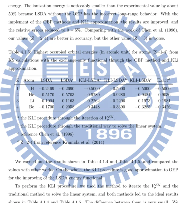
The exactly exchange-correlation functional is not yet known, so the approximation of exchange-correlation energy functionals is always one of the notable issues in DFT. The local spin-density approximation (LSDA) is widely employed. However, it has self-interaction such that the long-range behavior is not correct. The one of subjects in the present research is the correction to the self-interaction by the optimized effective potential (OEP) method and Krieger-Li-Iafrate (KLI) approximation (Krieger et al., 1992a). Based on the reliable KS calculation, we can establish the advanced techniques, OEP method and KLI approximation, and carry out the correctly total energies and highest occupied orbital energies for atomic system.
When an atomic or molecule system in intense field, the electronic response is highly non-linear. The non-linear process displays many interesting phenomena and applications. One consequence of them is the high-order harmonic generation (HHG) which converts the frequency of intense field into many integer multiples of the frequency. HHG spectra generally consist of a sharp decline, a plateau in which the harmonic intensity varies
weakly, and a sharp cut-off (see Figure 4.2.3). The maximum energy of harmonic photon is given by the cut-off law (Krause et al., 1992).
Ecut ≈ EI+ 3.17Up (1.0.1)
where EI is ionization energy, and Up is the pondermotive energy. The high-order
har-monic generation (HHG) is established as one of the best way to produce ultrashort coherent light (Midorikawa, 2011). It is worth researching with a theoretical aspect. In the present research, the other subject is the simulation of HHG of a hydrogen atom in the intense field. We directly solve the time-dependent Schr¨odinger equation to find the evolution of wave function and remark some features about HHG from the results. The results are also compared with the work (Tong and Chu, 1997b) to confirm the result. It is to build up our ability to deal with the time-dependent problems.
With the development of computer, the new device, graphics processing unit (GPU) accelerator and programming interface, OpenACC, are used in our computation. We perform the computation for the time iteration to simulate the HHG of a hydrogen atom in the intense field. It has an apparent effect on the computational speed, and the cost time is reduced to the acceptable range.
The necessarily numerical method for the present research are introduced in Chapter 2. Chapter 3 is a brief about density functional theory for the KS calculation. The result and discussion are in Chapter 4. From now on all of equations are in atomic unit. Following four fundamental constants are unity.
¯
h = e = me=
1 4πε0
Chapter 2
Methods
2.1
Quadratures and Grids
The integrations occur frequently in the inner product of two wave functions or an expan-sion in orthogonal basis. Its specific and non-uniform grids are also used in the generalized-pseudo spectral method throughout the numerical calculations in the present research. To numerical calculate these integrations, the quadrature and specific grids are necessary. Gauss-Legendre quadrature and Gauss-Legendre-Lobatto quadrature are introduced in this section.
2.1.1
Gaussian Quadrature
For the numerical integration, Gaussian quadrature has the highest accuracy in theory, but its grids and coefficients are hard to calculate. The general formula of Gaussian quadrature is b ∫ a w(x)f (x)dx =∑ i Wif (xi) (2.1.1)
where w(x) is the weighting function, xi are specific grids called Gauss nodes or
Gaus-sian grids, and Wi are the weights on the Gaussian grids. When the interval [a, b] and
weighting function w(x) are given, the Wi and xi are determined.
There are many typical forms for the interval [a, b] and weighting function w(x) derived from different orthogonal polynomials in (2.1.1). For a example, the interval [−1, 1] and weighting function 1/√1− x2 in common use are derived from Chebyshev polynomials of
2.1.2
Gaussian Grids and Weights
We only chose the [a, b] and w(x) based on the Legendre polynomials throughout the present research. For Legendre polynomials, the valid interval is [−1, 1]. The weighting function w(x) is a constant as follow
w(x) = 1 (2.1.2) In practice, the unity lets us avoid calculating the weighting function for the integral function. With the given interval [−1, 1] and weighting function w(x), there are three unique sets of Gaussian grids xi and weights Wi. We used two of them in calculation.
The first set is the roots of Legendre polynomial PN(x), x = cos θ, with degree N .
The roots can be numerically calculated by the recurrence relations, (A.0.3) and (A.0.4), and Newton’s method. The roots of PN(x) form following collocation points,
xi ∈ {x1, x2, . . . , xN−1, xN}. (2.1.3)
In this thesis, the set (2.1.3) of points is called Gauss-Legendre grids, abbreviated to GL grids. They are non-uniformly distributed over the abscissa and symmetric (or antisymmetry) to zero point. The relation between the polynomial degree N and the number of GL grids NGL is
NGL = N (2.1.4)
The weights Wi for GL grids are (Abramowitz and Stegun, 1972, p.887)
Wi =
2
(1− xi)[PN′ (x)]2
(2.1.5) The domain of GL grids is [−1, 1]. It is suitable for expressing the polar angle in spherical coordinate in discreteness without mapping.
The other set is the roots of the first derivative of Legendre polynomial PN′ (x), x = cos θ, with degree N . The roots can be numerically calculated by recurrence relations, (A.0.4) and (A.0.5) and Newton’s method. In addition, it includes the end points of interval [−1, 1]. The roots and end points form the collocation points,
xi ∈ {x0 =−1, x1, x2, . . . , xN−1, xN = 1} (2.1.6)
where x0 and xN are end points, and x1,· · · , xN−1 are the roots of PN′ (x). In this thesis,
Their distribution is the same as GL grid. The relation between the polynomial degree
N and the number of GLL grids NGLL′ is
NGLL′ = N + 1. (2.1.7)
The weights Wi for GLL grids are (Abramowitz and Stegun, 1972, p.888)
Wi =
2
N (N + 1)[PN(xi)]2
. (2.1.8)
Because of the inaccuracy close to the end points of interval, the subset of GLL grids was used more often than the GLL grids in actual calculation. The subset excluding the end points, x0 and xN, only has the roots of PN′ (x),
xi ∈ {x1, x2, ..., xN−1}. (2.1.9)
The relation between the polynomial degree N , the number of all GLL grids NGLL′ , and the number of this subset NGLL is
NGLL = N− 1 = NGLL′ − 2. (2.1.10)
2.1.3
Mapping Funciton
The GLL grids xi of which valid domain is [−1, 1] can not express the radius r of which
valid domain is [0,∞] in spherical coordinates. The connection of different domain is called mapping. To achieve mapping, it requires a function which is also called mapping
function.
Between the two intervals, x∈ [−1, +1] and r ∈ [0, ∞], there are two nonlinear map-ping, algebraic mapping and exponential mapmap-ping, to use. We only used algebraic mapping in the present research because the algebraic mapping is more accurate than exponential mapping in practice. The algebraic mapping is
r(x) = L1 + x + β
1− x + α (2.1.11) where α and β are constants to determine the boundaries, rmin and rmax. With x =−1,
r(−1) is the boundary rmin,
rmin = L
β
2 + α. (2.1.12)
With x = 1, r(1) is the boundary rmax,
rmax= L
2 + β
When α = β = 0, the interval [−1, 1] can be map to the interval [0, ∞].
The values of two constants α and β in (2.1.11) should be noted. The constant β may not be used and let itself be zero.
β = 0 (2.1.14)
The other constant α should be added and let itself be non-zero to avoid divergence of
r(x) at the last GLL point, r(1). r(x), rmin, and rmax with the given β are redefined as
r(x) = L 1 + x 1− x + α (2.1.15) rmin = 0 (2.1.16) rmax = L 2 α (2.1.17)
The other constant L in mapping functions, (2.1.11) and (2.1.15), is called length
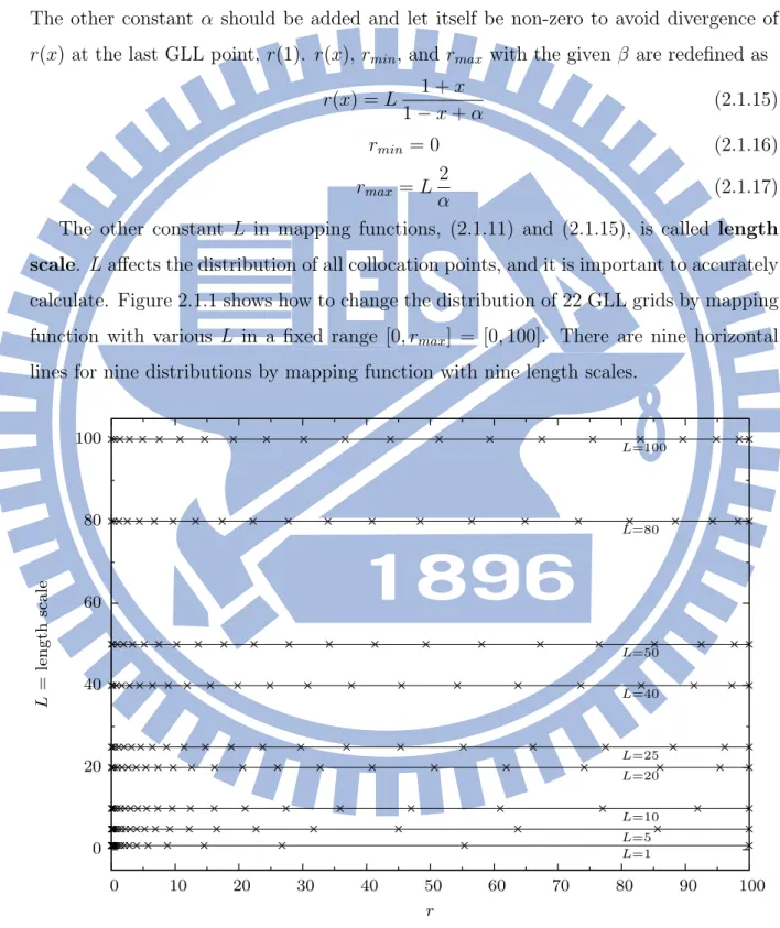
scale. L affects the distribution of all collocation points, and it is important to accurately
calculate. Figure 2.1.1 shows how to change the distribution of 22 GLL grids by mapping function with various L in a fixed range [0, rmax] = [0, 100]. There are nine horizontal
lines for nine distributions by mapping function with nine length scales.
0 20 40 60 80 100 0 10 20 30 40 50 60 70 80 90 100 L = length scale r L=1 L=5 L=10 L=20 L=25 L=40 L=50 L=80 L=100
Figure 2.1.1: Influence of various length scale L by mapping function on grid-point dis-tribution
L = 1 does not change the distribution. The distribution shows that the most grids
are close to the origin, r = 0, and very dense near the origin, r = 0. It can not correctly describe the shape of a function on the middle or far grids, and it may lead to inaccuracy calculation when L = 1. On increase of L, the influence of L on the distribution decreases gradually, and the distribution is changed a little. When L is over a value, the grids start to approach to the rmax.
In practice, the length scale L depends on the variation of function. With the adapted length scales for different problems, the grids can describe the functions well. In the present research, the most functions are the wave functions in stationary state. The wave functions oscillate near the nucleus and decay quickly, so we multiplied rmax/5 or rmax/10
to the mapping function r(x) as a length scale.
Map the interval [−1, 1] to interval [0, rmax] by the mapping function (2.1.15), and the
Gaussian quadrature requires a variable change,
r′(x) = d
dxr(x) = L
2 + α
(1− x + α)2, (2.1.18)
in term of x to work. The Gaussian quadrature with interval [−1, 1] and weighting function
w(x) = 1 becomes r∫max 0 f (r)dr =∑ i Wif (r(xi)) dr(xi) dx . (2.1.19)
where xi are GLL or GL grids, Wi are weights on GLL or GL grids.
More mapping functions that map finite interval to semi-infinite interval or infinite interval can be found in Canuto et al. (2007,§ 8.8 )
2.2
Generalized Pseudo-Spectral Method (GPS)
Generalized pseudo-spectral method (GPS) is to solve the ordinary differential equations (ODE) or partial differential equations (PDE). GPS uses a pseudo-spectral basis which is constructed by orthogonal polynomials to represent the functions in a differential equation on Gaussian grids. By GPS, ODE becomes an integration or eigenvalue problem. On the Gaussian grids and pseudo-spectral basis, it is easy to deal with the integration and eigenvalue problem. GPS plays a key role in the present research. This section and the next two sections provide the principles and its applications.2.2.1
Polynomial Interpolation and Cardinal Functions
Polynomial interpolation is one of interpolations methods. It is the generalization of linear interpolation which is the simplest interpolation. The Lagrange interpolation is one of algorithms to realize polynomial interpolation and better than other algorithms in time complexity.
The Lagrange interpolation is known that a unknown function f (x) with some given points xi is approximated by a polynomial p(x). In general, if there are N + 1 given
points, the unknown function f (x) is fitted by a degree-N polynomial pN(x) as follow
f (x)≈ pN(x) = N
∑
i=0
f (xi)gi(x) (2.2.1)
where gi(x) are cardinal functions. With these given points xj, the cardinal functions are
defined by gi(x) = N ∏ j=0 j̸=i x− xj xi− xj . (2.2.2)
In definition, it must satisfy following property,
gj(xi) = δij. (2.2.3)
The Lagrange interpolation with the given cardinal functions is also called cardinal
expansion or expansion in cardinal functions. The cardinal functions defined by
2.2.2
Cardinal Functions for Orthogonal Polynomials
By GLL grids and Legendre polynomials, define the cardinal functions gj(x) as follow
(Canuto et al., 1988, p.64) gj(x) =− 1 N (N + 1)PN(xj) (1− x2)P′ N(x) x− xj (2.2.4) Following paragraphs show that the cardinal functions (2.2.4) have the property (2.2.3).
When x = xi = xj on GLL grids, use a limit to approach.
lim x→xi gj(x) =− 1 N (N + 1)PN(xj) (1− x2 j)PN′ (xj) xj − xj (2.2.5) See both denominator and numerator are zero, so apply l’Hˆopital’s rule to the limit.
lim x→xi gj(x) = − 1 N (N + 1)PN(xj) [(1− x2)PN′ (x)]′ (x− xj)′ (2.2.6) With the relation (A.0.6) in appendix A,
lim x→xi gj(x) =− 1 N (N + 1)PN(xj) [−N(N + 1)PN(x)] 1 . (2.2.7)
The limit is a constant.
gj(xj) = − 1 N (N + 1)PN(xj) [−N(N + 1)PN(xj)] 1 = 1 (2.2.8) When x = xi ̸= xj on GLL grids, gj(xi) =− 1 N (N + 1)PN(xj) (1− x2i)PN′ (xi) xi− xj (2.2.9) Only the numerator is zero because (1−x2i) = 0, or PN′ (xi) = 0, and the other coefficients are not zero.
gj(xi) =− 1 N (N + 1)PN(xj) 0 xi− xj = 0 (2.2.10)
Combine two results, (2.2.8) and (2.2.10), and the cardinal functions satisfy the property (2.2.3).
2.2.3
Derivatives of Cardinal Functions
The cardinal expansion lets the operators in differential equation work on the cardinal functions to represent the operators in discrete variables. For the cardinal functions (2.2.4), its first and second derivatives which we applied in practice are analysed (Wang and Yan, 2012) and summarized (Telnov and Chu, 1999, appendix) in this subsection.
I From definition (2.2.4),
N (N + 1)PN(xj)(x− xj)gj(x) =−(1 − x2)PN′ (x). (2.2.11)
Differentiate both sides with respect to x.
N (N + 1)PN(xj)gj(x) + N (N + 1)PN(xj)(x− xj) dgj(x) dx =− d dx[(1− x 2)P′ N(x)] (2.2.12) Replace [(1− x2)PN′ (x)]′ by (A.0.6). N (N + 1)PN(xj)gj(x) + N (N + 1)PN(xj)(x− xj) dgj(x) dx = N (N + 1)PN(x) (2.2.13)
Eliminate the coefficient N (N + 1) occurring on both sides.
PN(xj)gj(x) + PN(xj)(x− xj) dgj(x) dx = PN(x) (2.2.14) When x = xi ̸= xj on GLL grids, PN(xj)gj(xi) + PN(xj)(xi− xj) dgj(xi) dx = PN(xi). (2.2.15)
gj(xi) = 0 because xi ̸= xj, and rearrange the equation.
dgj(xi) dx = 1 (xi− xj) PN(xi) PN(xj) (2.2.16)
II Take the derivatives of the terms on both sides of (2.2.14) with respect to x. 2PN(xj) dgj(x) dx + PN(xj)(x− xj) d2g j(x) dx2 = P ′ N(x) (2.2.17)
When x = xi = xj on GLL grids, and x̸= x0 ̸= xN,
2PN(xj) dgj(xj) dx + PN(xj)(xj − xj) d2gj(xj) dx2 = P ′ N(xj). (2.2.18)
(xj − xj) and PN′ (xj) are zero, and PN(xj) is not zero.
dgj(xj)
dx = 0 (2.2.19)
III When x = xi = xj = x0 =−1 on GLL grids, from (2.2.17),
2PN(−1) dgj(−1) dx + PN(−1)(−1 + 1) d2g j(−1) dx2 = P ′ N(−1) (2.2.20)
The second term is zero, and the PN(±1) and PN′ (±1) are given by (A.0.1) and (A.0.2)
in Appendix A.
2(−1)Ndgj(x0)
dx + 0 = (−1)
N +1N (N + 1)
Rearrange the equation.
dgj(x0)
dx =−
N (N + 1)
4 (2.2.22)
When x = xi = xj = xN = 1 on GLL grids, by the same way,
dgj(xN)
dx =
N (N + 1)
4 (2.2.23)
Following equation summarizes the formulae, (2.2.16), (2.2.19), (2.2.22), and (2.2.23), of the first derivative of the gj(x) on GLL grids.
dgj(xi) dx = g ′ j(xi) = d′ij PN(xi) PN(xj) (2.2.24) where d′ij = 1 xi− xj i̸= j 0 i = j ̸= 0 ̸= N −N (N + 1) 4 (i, j) = (0, 0) N (N + 1) 4 (i, j) = (N, N ) (2.2.25)
The calculation of the second derivative of the gj(x) on GLL grids based on its first
derivative on GLL grids. Following paragraphs are the derivation of the formulae for the second derivative of gj(x) on GLL grids.
I When x = xi ̸= xj on GLL grids, and xi ̸= 0 ̸= N, from (2.2.17),
2PN(xj) dgj(xi) dx + PN(xj)(xi− xj) d2gj(xi) dx2 = P ′ N(xi). (2.2.26)
PN′ (xi) is zero, and the gj′(xi) where xi ̸= xj is given by (2.2.16).
2PN(xi)
xi− xj
+ PN(xj)(xi− xj)
d2gj(xi)
dx2 = 0 (2.2.27)
Rearrange the equation.
d2g j(xi) dx2 =− 2 (xi− xj)2 PN(xi) PN(xj) (2.2.28)
II Differentiate both sides of (2.2.17) with respect to x. 3PN(x) d2gj(x) dx2 + (x− xj)PN(xj) d3gj(x) dx3 = P ′ N(x) (2.2.29)
When x = xi = xj on GLL grids, xi = xj ̸= x0, and xi = xj ̸= xN,
3PN(xj) d2gj(xj) dx2 + (xj − xj)PN(xj) d3gj(xj) dx3 = P ′ N(xj). (2.2.30)
The second term is zero because of its coefficient, (xj−xj) = 0. With the relation (A.0.10) in Appendix A, 3PN(xj) d2gj(xj) dx2 + 0 = N (N + 1)PN(xj) (x2 j − 1) . (2.2.31)
Rearrange the equation.
d2g j(xj) dx2 = N (N + 1) (x2 j − 1) PN(xj) PN(xj) =−N (N + 1) 3(1− x2 j) (2.2.32) Following equation summarizes the formulae, (2.2.28), (2.2.32), and remaining formu-lae that we did not use in the present research.
d2g j(xi) dx = g ′′ j(xi) = d′′ij PN(xi) PN(xj) (2.2.33) where d′′ij = − 2 (xi− xj)2 i̸= j (i, j) ̸= (0, N) ̸= (N, 0) −N (N + 1) 3(1− x2 j) i = j (i, j)̸= (0, 0) ̸= (N, N) N (N + 1)− 2 4 (i, j) = (0, N ) = (N, 0) N (N + 1)[N (N + 1)− 2] 24 (i, j) = (0, 0) = (N, N ) (2.2.34)
Pseudo-spectral methods are closely related to the spectral methods. The famous publications, Peyret (2002) and Canuto et al. (2007), about spectral methods also offer the materials for pseudo-spectral methods.
2.2.4
Differential Matrix
(2.2.24) points out a direct application to numerical differential. Assume that f (r(x)) is a function which maps from the r domain to the x domain. Take the derivative with respect to r. df (r(x)) dr = dx dr(x) df (r(x)) dx (2.2.35)
Expand f (x) in the cardinal functions (2.2.4).
df (r(x)) dr = 1 r′(x) ∑ j dgj(x) dx f (r(xj)) (2.2.36) Discretize x on GLL grids, x = xi. df (r(xi)) dr = 1 r′(xi) ∑ j dgj(xi) dx f (r(xj)) (2.2.37)
Equation (2.2.37) is a matrix-vector product. With all GLL grids, xi and xj, the g′j(xi)
with the coefficient [r′(xi)]−1 form a (N + 1)× (N + 1) matrix D. The element Dij of the
matrix D is Dij = 1 r′(xi) dg(xi) dx = 1 r′(xi) d′ijPN(xi) PN(xj) (2.2.38) where d′ij is given by (2.2.25). If f (r(xi)) is given, the matrix-vector product of Dij and
f (r(xj)) can directly give the derivatives f′(r(xi)) with respect to r without other
tech-niques. The work of D is the same as a differential operator, and D is called differential
matrix.
When more grids are used in a numerical calculation, more round-errors occur in numerically calculating the derivatives by the differential matrix D. Bayliss et al. (1995) offer a technique to reduce the round-off errors to make the derivatives more accurate. It is easy to derive the technique. Let a operator d/dx work on a constant function, f (x) = c where c is a constant.
d
dxf (x) = d
dxc = 0 (2.2.39)
Discretize x on GLL grids, and substitute the operator by the differential matrix D. ∑
j
Dijf (xj) = 0 (2.2.40)
Let the diagonal elements of D be correction terms.
Diif (xi) =−
∑
j i̸=j
Dijf (xj) (2.2.41)
Divide both sides by c, and the diagonal elements now become
Dii =−
∑
j j̸=i
Dij. (2.2.42)
The off-diagonal elements follow the original definition. The diagonal elements (2.2.42) eliminate the round-off errors of the off-diagonal elements. The differential matrix with the correction is denoted Dcor.
For an example of which derivative is analysis and easy to calculate,
f (r(x)) = exp(−r(x)). (2.2.43) We numerically calculated its first and second derivative with respect to r by the differ-ential matrix D.
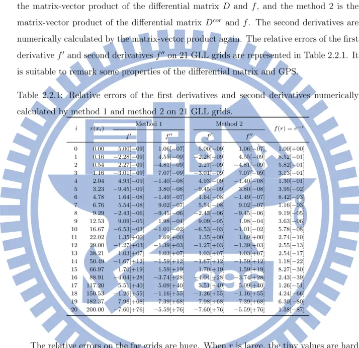
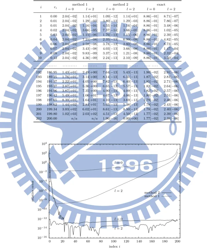
By the mapping function (2.1.15) with L = 20, the valid interval of r is [0, 200]. 21 GLL grids are used in the numerical calculation, and 21 derivatives are numerically calculated by method 1 and method 2. For the numerical differential, the method 1 is the matrix-vector product of the differential matrix D and f , and the method 2 is the matrix-vector product of the differential matrix Dcor and f . The second derivatives are numerically calculated by the matrix-vector product again. The relative errors of the first derivative f′ and second derivatives f′′ on 21 GLL grids are represented in Table 2.2.1. It is suitable to remark some properties of the differential matrix and GPS.
Table 2.2.1: Relative errors of the first derivatives and second derivatives numerically calculated by method 1 and method 2 on 21 GLL grids.
i r(xi) Method 1 Method 2 f (r) = e−r f′ f′′ f′ f′′ 0 0.00 5.00[−09] 1.06[−07] 5.00[−09] 1.06[−07] 1.00[+00] 1 0.16 −2.28[−09] 4.55[−09] −2.28[−09] 4.55[−09] 8.52[−01] 2 0.54 2.27[−09] −4.81[−09] 2.27[−09] −4.81[−09] 5.82[−01] 3 1.16 −3.01[−09] 7.07[−09] −3.01[−09] 7.07[−09] 3.13[−01] 4 2.04 4.93[−09] −1.40[−08] 4.93[−09] −1.40[−08] 1.30[−01] 5 3.23 −9.45[−09] 3.80[−08] −9.45[−09] 3.80[−08] 3.95[−02] 6 4.78 1.64[−08] −1.49[−07] 1.64[−08] −1.49[−07] 8.42[−03] 7 6.76 5.54[−08] 9.02[−07] 5.54[−08] 9.02[−07] 1.16[−03] 8 9.29 −2.43[−06] −9.45[−06] −2.43[−06] −9.45[−06] 9.19[−05] 9 12.53 9.09[−05] 1.98[−04] 9.09[−05] 1.98[−04] 3.63[−06] 10 16.67 −6.53[−03] −1.01[−02] −6.53[−03] −1.01[−02] 5.78[−08] 11 22.02 1.35[+00] 1.69[+00] 1.35[+00] 1.69[+00] 2.74[−10] 12 29.00 −1.27[+03] −1.39[+03] −1.27[+03] −1.39[+03] 2.55[−13] 13 38.21 1.03[+07] 1.03[+07] 1.03[+07] 1.03[+07] 2.54[−17] 14 50.49 −1.67[+12] −1.59[+12] −1.67[+12] −1.59[+12] 1.18[−22] 15 66.97 1.70[+19] 1.59[+19] 1.70[+19] 1.59[+19] 8.27[−30] 16 88.91 −4.04[+28] −3.74[+28] −4.04[+28] −3.74[+28] 2.43[−39] 17 117.20 5.51[+40] 5.09[+40] 5.51[+40] 5.09[+40] 1.26[−51] 18 150.53 −1.26[+55] −1.16[+55] −1.26[+55] −1.16[+55] 4.24[−66] 19 182.37 7.98[+68] 7.39[+68] 7.98[+68] 7.39[+68] 6.30[−80] 20 200.00 −7.60[+76] −5.59[+76] −7.60[+76] −5.59[+76] 1.38[−87]
The relative errors on the far grids are huge. When r is large, the tiny values are hard to be described by the pseudo-spectral basis. It does not affect the numerical calculation because the order of magnitude is too small. If the cases is that exp(−r) fast decay when
r increase, the values on the grids near the point, r = 0, are leading terms, and the values
on the grids far from the point, r = 0, can be ignored.
As listed in Table 2.2.1, the first derivatives f′ and second derivatives f′′ numerically calculated by the method 1 and 2 are almost identical to each other. It is evident that the accuracy of f′′ is less than the accuracy of f′ especially at the point r(x0). The round-off
of Bayliss et al. (1995). The correction to round-off errors on the less grids is not easily obvious in Table 2.2.1.
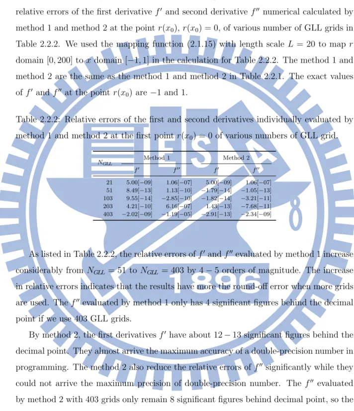
To show the efficacy of the technique for reducing the round-off errors, we present the relative errors of the first derivative f′ and second derivative f′′ numerical calculated by method 1 and method 2 at the point r(x0), r(x0) = 0, of various number of GLL grids in
Table 2.2.2. We used the mapping function (2.1.15) with length scale L = 20 to map r domain [0, 200] to x domain [−1, 1] in the calculation for Table 2.2.2. The method 1 and method 2 are the same as the method 1 and method 2 in Table 2.2.1. The exact values of f′ and f′′ at the point r(x0) are −1 and 1.
Table 2.2.2: Relative errors of the first and second derivatives individually evaluated by method 1 and method 2 at the first point r(x0) = 0 of various numbers of GLL grid.
NGLL Method 1 Method 2 f′ f′′ f′ f′′ 21 5.00[−09] 1.06[−07] 5.00[−09] 1.06[−07] 51 8.49[−13] 1.13[−10] −1.79[−14] −1.05[−13] 103 9.55[−14] −2.85[−10] −1.82[−14] −3.21[−11] 203 4.21[−10] 6.16[−07] 1.43[−13] −7.68[−11] 403 −2.02[−09] −1.19[−05] −2.91[−13] −2.34[−09]
As listed in Table 2.2.2, the relative errors of f′and f′′evaluated by method 1 increase considerably from NGLL = 51 to NGLL = 403 by 4− 5 orders of magnitude. The increase
in relative errors indicates that the results have more the round-off error when more grids are used. The f′′ evaluated by method 1 only has 4 significant figures behind the decimal point if we use 403 GLL grids.
By method 2, the first derivatives f′ have about 12− 13 significant figures behind the decimal point. They almost arrive the maximum accuracy of a double-precision number in programming. The method 2 also reduce the relative errors of f′′ significantly while they could not arrive the maximum precision of double-precision number. The f′′ evaluated by method 2 with 403 grids only remain 8 significant figures behind decimal point, so the number of grid should be adequate. On the whole, the technique offered by Bayliss et al. (1995) has beneficial effect on reducing the round-off errors.
2.3
Application of GPS to Schr¨
odinger Equation
The time-independent Schr¨odinger equation, which is abbreviated to SE, readsˆ Hψ(r) =− ¯h 2 2m∇ 2 ψ(r) + V ψ(r) = Eψ(r) (SI). (2.3.1) Suppose the external potential V only depends on radius r in spherical coordinates. By separation of variables and variable change, u(r) = rR(r), the radial equation in atomic unit is −1 2 d2 dr2u(r) + [ l(l + 1) 2r2 + V (r)]u(r) = Eu(r). (2.3.2)
By the expansion in spherical harmonics, we only solved the radial equation.
The first application of GPS is a solver for Schr¨odinger equation. In this section, remove the undesirable feature due to the non-linear mapping at first, and construct the Hamiltonian matrix by GPS. The technique to symmetrize the Hamiltonian matrix is also introduced in this section. We solved the SE of a hydrogen atom in the last subsection.
2.3.1
Radial Equation Represented in x Domain
For the application of GPS, discretize u(r) on the GLL grids by the mapping function (2.1.15). The non-linear mapping of the second derivative of u(r(x)) with respect to r leads to the first derivative of u(r(x)) with respect to x occurring in the radial equa-tion. The elimination of the undesirable first derivative with respect to x is necessary for symmetrizing the Hamiltonian matrix. This subsection represents how to eliminate the redundant derivative.
Mapping u(r) from r domain to x domain, the first derivative of u(r) with respect to
r is d dru(r(x)) = dx dr d dxu(r(x)) = 1 r′ d dxu(r(x)). (2.3.3)
Take a derivative of the terms on both sides with respect to r again.
d2 dr2u(r(x)) = 1 (r′)2[− r′′ r′ d dx + d2 dx2]u(r(x)) (2.3.4)
With (2.3.4), the radial equation (2.3.2) becomes 1 2(r′)2[− r′′ r′ d dx + d2 dx2]u(r(x)) + [ l(l + 1) 2r2 + V (r)]u(r(x)) = Eu(r(x)). (2.3.5)
To eliminate the first derivative, the variable change makes
u(r) = (dr(x) dx )
C
where the f (x) is a function which can be expanded in the cardinal functions (2.2.4) in x domain, and the exponent C is a undetermined coefficient. Determine C by substituting (2.3.6) into (2.3.4). d2u(r(x)) dr2 = 1 (r′)2 [ −r′′ r′ ( C(r′)C−1r′′+ (r′)C d dx ) +(C(C− 1)(r′)C−2(r′′)2 + C(r′)C−1r′′′+ 2C(r′)C−1r′′ d dx + (r ′)C d2 dx2 )] f (x) (2.3.7)
Rearrange and bracket the first derivatives.
d2u(r(x)) dr2 = 1 (r′)2 [ C(C− 2)(r′)C−2(r′′)2+ C(r′)C−1r′′′ +(2C(r′)C−1r′′− (r′)C−1r′′) d dx + (r ′)C d2 dx2 ] f (x) (2.3.8)
Let the coefficient of the first derivative be zero
2C(r′)C−1r′′− (r′)C−1r′′ = 0 (2.3.9) Calculate the C.
C = 1
2 (2.3.10)
The exponent C is determined now.
With the given C, observe these terms without the first derivatives and second deriva-tives in (2.3.8). C(C− 2)(r′)C−2(r′′)2+ C(r′)C−1r′′′ =−3 4(r ′)−3 2(r′′)2 +1 2(r ′)−1 2r′′′ (2.3.11)
r(x) is given, and its derivatives, r′(x), r′′(x), and r′′′(x), are easy to derive.
C(C − 2)(r′)C−2(r′′)2+ C(r′)C−1r′′′ =− 3 4[ (1− x + α)2 2 ] 3 2[ 4 (1− x + α)3] 2+1 2[ (1− x + α)2 2 ] 1 2 12 (1− x + α)4 =− 3 4 (1− x + α)3 2√2 16 (1− x + α)6 + 1 2 (1− x + α) √ 2 12 (1− x + α)4 = 0 (2.3.12)
The given C also lets the summation be zero.
The variable change (2.3.6) with the given exponent C, C = 1/2, is
By the variable change (2.3.13), the second derivative of u(r(x)) with respect to r can be found from (2.3.8), (2.3.9), and (2.3.12) with the given C,
d2u(r(x)) dr2 = 1 (r′)2[0 + 0 + (r ′)1 2 d 2 dx2]f (x) = (r ′)−3 2d 2f (x) dx2 , (2.3.14)
and the radial equation (2.3.2) becomes
−1 2(r ′)−3 2d 2f (x) dx2 + [ l(l + 1) 2r2 + V (r)](r ′)1 2f (x) = E(r′) 1 2f (x). (2.3.15)
2.3.2
Construction and Symmetrization of Hamiltonian Matrix
The discretization of the differential operator by GPS and symmetrization of Hamiltonian matrix are introduced in this subsection.
Following paragraph describes how to apply GPS to the discretization of the differ-ential operator. For the function f (x) in (2.3.15), expand f (x) in the cardinal functions
gj(x) defined by (2.2.4),
f (x) =∑
j
gj(x)f (xj), (2.3.16)
and the differential operator with respect to x works on the cardinal functions gj(x) but
not f (xj). d2f (x) dx2 = ∑ j d2g(x) dx2 f (xj) (2.3.17)
With (2.3.16) and (2.3.17), the radial equation (2.3.15) is on the pseudo-spectral basis.
− 1 2[r ′(x i)]− 3 2 ∑ j d2gj(x) dx2 f (xj) + ( l(l + 1) 2[r(x)]2 + V (r(x)) ) [r′(x)]12 ∑ j gj(x)f (xj) = E [r′(x)]12 ∑ j gj(x)f (xj) (2.3.18)
Subsequently discretize x on GLL grids, x = xi.
− 1 2[r ′(x i)]− 3 2 ∑ j d2g j(xi) dx2 f (xj) + ( l(l + 1) 2[r(xi)]2 + V (r(x)))[r′(xi)] 1 2 ∑ j gj(xi)f (xj) = E [r′(xi)] 1 2 ∑ j gj(xi)f (xj) (2.3.19) Both sides of (2.3.19) are divided by [r′(xi)]
1
out of the square brackets. ∑ j [ −1 2[r ′(x i)]−2 d2g j(xi) dx2 + ( l(l + 1) 2[r(xi)]2 + V (r(xi)) ) gj(xi) ] f (xj) = E ∑ j gj(xi)f (xj) (2.3.20)
The GPS has been performed, and whole equation is represented by discrete variables, xi
and xj, in x domain.
In (2.3.20), the square bracket is a Hamiltonian matrix H. The H is non-symmetric due to the coefficient [r′(xi)]−2 of the second derivative. The non-symmetry leads to
generalized eigenvalue problem of which eigenvalues and eigenfunction may have complex numbers. The rest in the subsection is to symmetrize the H to avoid the complex number occurring in solutions and speed up in solving the eigenvalue problem.
Substitute (2.2.3) and (2.2.33) into (2.3.20). ∑ j [ −1 2[r ′(x i)]−2d′′ij PN(xi) PN(xj) +( l(l + 1) 2[r(xi)]2 + V (r(xi)) ) δij ] f (xj) = E ∑ j δijf (xj) (2.3.21) f (xj) multiplied by r′(xj)[PN(xj)]−1 becomes Aj. ∑ j [ −1 2[r ′(x i)]−2d′′ij PN(xi) r′(xj) +( l(l + 1) 2[r(xi)]2 + V (r(xi)) ) δij PN(xj) r′(xj) ] Aj = E ∑ j δij PN(xj) r′(xj) Aj (2.3.22) where Aj = r′(xj)f (xj) PN(xj) . (2.3.23)
Because the property of δij, let
PN(xj) r′(xj) δij = PN(xi) r′(xi) δij.
Eliminate the same coefficient, PN(xi)[r′(xi)]−1, on both sides.
∑ j [ −1 2[r ′(x i)]−1d′′ij[r′(xj)]−1+ ( l(l + 1) 2[r(xi)]2 + V (r(xi)) ) δij ] Aj = E ∑ j δijAj (2.3.24)
Because of δij, the term, i = j, remains on the right side of the equation. ∑ j [ −1 2[r ′(x i)]−1d′′ij[r′(xj)]−1+ ( l(l + 1) 2[r(xi)]2 + V (r(xi)) ) δij ] Aj = E Aj (2.3.25)
The terms in the square brackets form a symmetric Hamiltonian matrix H. The elements of the H are Hij =− 1 2[r ′(x i)]−1d ′′ ij[r′(xj)]−1+ ( l(l + 1) 2[r(xi)]2 + V (r(xi)) ) δij. (2.3.26)
The centrifugal term and V (r(xi)) only occur on the diagonal elements of the H. (2.3.25)
is a symmetric eigenvalue problem. In physics, the Dirichlet boundary conditions,
A0 = AN = 0, (2.3.27)
are usually used for the wave functions in quantum mechanics. We used the subset of GLL grids (2.1.9) that excludes the end points, x0 = −1 and xN = 1, to solve (2.3.25), and
found the eigenvalues {En|n = 1, . . . , N − 1} and the eigenstates {Aj|j = 1, . . . , N − 1}.
There are a brief of this section in Telnov and Chu (1999), and a similar work (Wang et al., 1994) that applies GPS to a Schr¨odinger equation.
2.3.3
Example: Hydrogen Atom
GPS with dense mesh is a good method to treat a system with the central potential. The dense mesh can effectively describe the variation near the point, r = 0, in the system. It lets the numerical calculation for the system by GPS be more accurate. For a example, we solved the Schr¨odinger Equation (SE) of a hydrogen atom that only has Coulomb potential.
The hydrogen atom is the simplest atomic problem. The single electron faces the bare Coulomb potential, V (r) =− 1 4πε0 e2 r (SI) =− 1 r, (2.3.28)
of nucleus. From (2.3.1), the full SE of the electron with potential (2.3.28) under the assumption of infinite nucleus mass reads
[−1 2∇
2− 1
r]ψ(r) = Eψ(r) (2.3.29)
The equation is analytically solvable. For bound states, the eigenvalues are
En(l) =−
1
and the eigenfunctions,
ψ(r) = Rn,l(r)Yl,m(θ, ϕ), (2.3.31)
are composed of the radial and angular parts. The solutions of the angular part are spherical harmonics Yl,m(θ, ϕ), and the solutions of the radial part are
Rn,l(r) = Nn,lexp(− r n)( 2r n ) lL2l+1 n−l−1( 2r n ) (2.3.32)
where Nn,l is the normalization constant, and L2l+1n−l−1 is associated Laguerre polynomials.
(2.3.30) and (2.3.32) are the theoretical formulae to compare with numerical results. For the numerical calculation, we suppose the angular part is given and only solve the radial equation (2.3.2) with the potential (2.3.28),
−1 2 d2 dr2u(r) + [ l(l + 1) 2r2 − 1 r]u(r) = Eu(r). (2.3.33)
The radial equation of discretization is given by (2.3.25). ∑ j [ −1 2[r ′(x i)]−1d′′ij[r′(xj)]−1+ ( l(l + 1) 2[r(xi)]2 − 1 r(xi) ))δij ] Aj = E Aj (2.3.34)
In programming, the eigenvalue problem is solved by the library, LAPACK, built in the MKL (Math Kernel Library) which is developed and optimized by Intel. The numeri-cal results are the eigenvalues and eigenfunctions. From the eigenfunctions, the radial functions are Rn,l(r(xj)) = AjPN(xj) r(xj) √ r′(xj) . (2.3.35)
Note that the Rn,l(r(xj)) are not normalized yet.
We discretized r on 101 GLL grids that exclude end points, x0 = −1 and xN = 1,
by the mapping function (2.1.15) with the length scale, L = 10. The maximum radius is
rmax = 100 a.u..
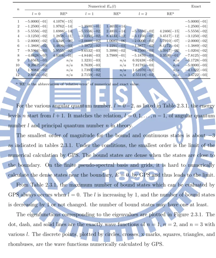
With the 101× 101 Hamiltonian matrix, 101 eigenvalues should be carried out. Table 2.3.1 gives the first 12 eigenvalues of (2.3.34) with angular quantum numbers, l = 0− 2. On the 101 eigenvalues, only 8 eigenvalues are positive numbers, and the rest are negative numbers. The negative and positive eigenvalues are the bound and continuous states of hydrogen atom. The analysis formula of energy levels is only used for the the bound states, so the relative errors of continuous states and exact values are denoted the abbreviation of ”not applicable”.
Table 2.3.1: Energy levels of neutral hydrogen atom from the solution of radial equation with angular quantum numbers, l = 0− 2, by GPS method.
n Numerical En(l) Exact l = 0 REa l = 1 REa l = 2 REa 1 −5.0000[−01] 4.1078[−15] −5.0000[−01] 2 −1.2500[−01] 1.9762[−14] −1.2500[−01] 1.4655[−14] −1.2500[−01] 3 −5.5556[−02] 1.6986[−14] −5.5556[−02] 2.4855[−14] −5.5556[−02] 4.2466[−15] −5.5556[−02] 4 −3.1250[−02] 1.2858[−11] −3.1250[−02] 8.4733[−12] −3.1250[−02] 3.4517[−12] −3.1250[−02] 5 −2.0000[−02] 1.4248[−06] −2.0000[−02] 1.0685[−06] −2.0000[−02] 5.7910[−07] −2.0000[−02] 6 −1.3868[−02] 1.4696[−03] −1.3872[−02] 1.2291[−03] −1.3877[−02] 8.4172[−04] −1.3889[−02] 7 −9.5964[−03] 5.9555[−02] −9.6532[−03] 5.3990[−02] −9.7560[−03] 4.3917[−02] −1.0204[−02] 8 −4.6628[−03] 4.0316[−01] −4.8446[−03] 3.7989[−01] −5.1876[−03] 3.3599[−01] −7.8125[−03]
9 1.6561[−03] n/a 1.3231[−03] n/a 6.92438[−04] n/a −6.1728[−03]
10 9.2667[−03] n/a 8.7639[−03] n/a 7.81785[−03] n/a −5.0000[−03]
11 1.8084[−02] n/a 1.7393[−02] n/a 1.61070[−02] n/a −4.1322[−03]
12 2.8055[−02] n/a 2.7159[−02] n/a 2.55118[−02] n/a −3.4722[−03]
a’RE’ is the abbreviation of ’relative error’ of numerical and exact value.
For the various angular quantum number, l = 0−2, as listed in Table 2.3.1, the energy levels n start from l + 1. It matches the relation, l = 0, 1, . . . , n− 1, of angular quantum number l and principal quantum number n in theory.
The smallest order of magnitude for the bound and continuous states is about −3 as indicated in tables 2.3.1. Under the conditions, the smallest order is the limit of the numerical calculation by GPS. The bound states are dense when the states are close to the boundary. On the finite pseudo-spectral basis and grids, it is hard to numerically calculate the dense states near the boundary, E = 0, by GPS and thus leads to the limit. From Table 2.3.1, the maximum number of bound states which can be evaluated by GPS always occurs when l = 0. The l is increasing by 1, and the number of bound states is decreasing by 1 or not changed. the number of bound states may have one at least.
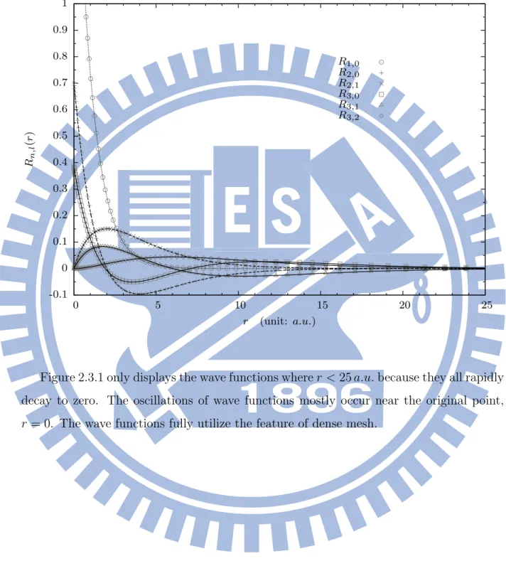
The eigenfunctions corresponding to the eigenvalues are plotted in Figure 2.3.1. The dot, dash, and solid lines are the exactly wave functions of n = 1, n = 2, and n = 3 with various l. The discrete points, plotted by circles, crosses, x marks, squares, triangles, and rhombuses, are the wave functions numerically calculated by GPS.
Figure 2.3.1: Radial function of a neutral hydrogen atom evaluated by GPS and theoretical formulae. The line is exact, and the points are numerical results.
-0.1 0 0.1 0.2 0.3 0.4 0.5 0.6 0.7 0.8 0.9 1 0 5 10 15 20 25 Rn,l (r ) r (unit: a.u.) R1,0 R2,0 R2,1 R3,0 R3,1 R3,2
Figure 2.3.1 only displays the wave functions where r < 25 a.u. because they all rapidly decay to zero. The oscillations of wave functions mostly occur near the original point,
2.4
Application of GPS on Poisson’s Equation
The Hartree potential VH(r) is a model that approximate the electrostatic interaction
of a electron due to all the other electrons in a system. The model assumes that the summation of state of individual electron is straightforward to construct the charge density distribution ρ(r). By integration of ρ(r) over all space, the VH(r) is
VH(r) =
∫
ρ(r′)
|r − r′|dr′. (2.4.1)
It is not easy to directly calculate the integration due to the|r−r′|−1, so the other method to calculate the VH(r) is necessary. The VH(r) satisfies the Poisson’s equation by Gauss
law.
∇2
VH(r) =−4πρ(r) (2.4.2)
Through solving the Poisson’s equation, the VH(r) can be found.
The second application of GPS is a solver for Poisson’s equation. The main body of this section is the discretization of the derivatives by GPS and construction of the the system equation. The boundary conditions can correct the solver, and make the calculation more accurate. The end of this section is a example.
2.4.1
Separation of Radial Part from Poisson’s Equation
The Poisson’s equation in atomic unit reads
∇2V (r) =−4πρ(r) (2.4.3)
where V (r) is the potential due to the source ρ(r), and ρ(r) is the electric charge distri-bution. Expand both V (r) and ρ(r) in spherical harmonics Yl,m(θ, ϕ).
V (r) =∑ l ∑ m Vl,m(r)Yl,m(θ, ϕ) (2.4.4) ρ(r) =∑ l ∑ m ρl,m(r)Yl,m(θ, ϕ) (2.4.5)
Assume that ρ(r) is azimuthal symmetry. The ρ(r) is independent of ϕ, and let m = 0 in the expansion. V (r) =∑ l Vl(r)Yl,0(θ, ϕ) = ∑ l ul(r) r Yl,0(θ, ϕ) (2.4.6) ρ(r) =∑ l ρl(r)Yl,0(θ, ϕ) (2.4.7)
Substitute the expansions of V (r) and ρ(r), (2.4.7) and (2.4.6), into Poisson’s equation (2.4.3). ∑ l ∇2 [ ul(r) r Yl,0(θ, ϕ) ] =−4π∑ l ρl(r)Yl,0(θ, ϕ) (2.4.8) Because Yl,0(θ, ϕ) = √ 2l + 1 4π Pl(x) (2.4.9)
where x = cos θ, the differential operators with respect to ϕ have no work, and (2.4.8) becomes ∑ l [ Yl,0(θ, ϕ) 1 r2 d dr ( r2 d dr( ul(r) r ) ) + (ul(r) r ) 1 r2sin θ d dθ ( sin θdYl,0(θ, ϕ) dθ )] =− 4π∑ l ρl(r)Yl,0(θ, ϕ) (2.4.10)
Yl,0(θ, ϕ) are the eigenfunctions of the angular momentum operator L2, so the angular
momentum operator L2, which works on its eigenfunctions Y
l,0(θ, ϕ), can be replaced by its eigenvalue−l(l + 1). ∑ l [ Yl,0(θ, ϕ) r d2ul(r) dr2 − ( ul(r) r ) l(l + 1) r2 Yl,0(θ, ϕ) ] =−4π∑ l ρl(r)Yl,0(θ, ϕ) (2.4.11)
Take Yl,0(θ, ϕ) out of the square brackets, and multiply r to both sides.
∑ l [ d2u l(r) dr2 − l(l + 1) r2 ul(r) ] Yl,0(θ, ϕ) =−4πr ∑ l ρl(r)Yl,0(θ, ϕ) (2.4.12)
The coefficients of Yl,0(θ, ϕ) provide
d2ul(r)
dr2 −
l(l + 1)
r2 ul(r) =−4πrρl(r) (2.4.13)
(2.4.13) is one of partially radial equations.
2.4.2
Construction of System of Linear Equations
Remaining steps are the discretization of the partially radial equation (2.4.13). Apply variable change, (2.3.13) and (2.3.14), to (2.4.13).
[r′(x)]−32d 2f l(x) dx2 − l(l + 1) r2 [r ′(x)]1 2fl(x) =−4πrρl(r) (2.4.14)
This equation is mapped to x domain. Multiply [r′(x)]3/2 to both sides of (2.4.14), and the coefficient of fl′′(x) becomes unity,
d2f l(x) dx2 − l(l + 1)( r′(x) r(x)) 2f l(x) =−4πr(x)[r′(x)] 3 2ρl(r). (2.4.15)
Apply GPS to discretize the fl(x) on the pseudo-spectral basis. Expand fl(x) in the cardinal functions (2.2.4). ∑ j [ d2g j(x) dx2 − l(l + 1)( r′(x) r(x)) 2g j(x) ] fl(xj) =−4πr(x)[r′(x)] 3 2ρl(r) (2.4.16) Discretize x on GLL grid, x = xi. ∑ j [ d2gj(xi) dx2 − l(l + 1)( r′(xi) r(xi) )2gj(xi) ] fl(xj) = −4πr(xi)[r′(xi)] 3 2ρ l(r(xi)) (2.4.17)
gj′′(xi) and gj(xi) are given by (2.2.24) and (2.2.33).
∑ j [ d′′ijPN(xi) PN(xj) − l(l + 1)(r′(xi) r(xi) )2δij ] fl(xj) = −4πr(xi)[r′(xi)] 3 2ρl(r(xi)) (2.4.18)
Inserting PN(xi)[PN(xj)]−1 to δij as a coefficient does not affect this equation because of
the property of δij. ∑ j [ d′′ijPN(xi) PN(xj) − l(l + 1)(r′(xi) r(xi) )2δij PN(xi) PN(xj) ] fl(xj) = −4πr(xi)(r′(xi)) 3 2ρ l(r(xi)) (2.4.19) Take [PN(xj)]−1 out the square brackets, and eliminate PN(xi) on both sides.
∑ j [ d′′ij − l(l + 1)(r ′(x i) r(xi) )2δij ] fl(xj) PN(xj) =−4πr(xi)[r′(xi)] 3 2ρl(r(xi)) PN(xi) (2.4.20)
With all GLL grids{xi|i = 0, 1, · · · , N}, the partially radial equations form a system of
linear equations, D0,0 D0,1 · · · D0,N−1 D0,N D1,0 D1,1 · · · D0,N−1 D1,N .. . ... . .. ... ... DN−1,0 DN−1,1 · · · DN−1,N−1 DN−1,N DN,0 DN,1 · · · DN,N DN,N a0 a1 .. . aN−1 aN = b0 b1 .. . bN−1 bN (2.4.21) where Dij = d′′ij − l(l + 1)( r′(xi) r(xi) )2δij, (2.4.22) aj = fl(xj) PN(xj) , (2.4.23) bi =−4πr(xi)[r′(xi)] 3 2ρl(r(xi)) PN(xi) . (2.4.24)
If all aj are carried out directly from the linear system (2.4.21) without any correction,
the inaccuracy is unavoidable because boundary the conditions, a0 and aN, are unknown.
2.4.3
Determination of Boundary Conditions
This subsection represents the numerical calculation of the boundary conditions by Gaus-sian quadrature.
When the electric charge distribution ρ(r) is given, the potential can be calculated by the integration over all space,
V (r) =
∫
ρ(r′)
|r − r′|d3r′. (2.4.25)
The expansion of V (r) and ρ(r) in spherical harmonics are given by (2.4.6) and (2.4.7). ∑ l′ ul′(r) r Yl′,0(θ, ϕ) = ∑ l′ ∫ ρl′(r′)Yl′,0(θ′, ϕ′) |r − r′| d 3 r′ (2.4.26)
The fraction |r − r′|−1 can also be expanded in the spherical harmonic functional space. 1 |r − r′| = ∑ l ∑ m 4π 2l + 1 rl< rl+1> Yl,m∗ (θ′, ϕ′)Yl,m(θ, ϕ) (2.4.27)
With the expansion of |r − r′|−1, (2.4.26) becomes ∑ l′ ul′(r) r Yl′,0(θ, ϕ) =∑ l′,l,m 4π 2l + 1Yl,m(θ, ϕ) ∫ rl< r>l+1 ρl(r′)r′2dr′ ∫ Yl,m∗ (θ′, ϕ′)Yl′,0(θ′, ϕ′)dΩ′ (2.4.28)
The integration of the production of two spherical harmonics is analysis by the orthogo-nality of spherical harmonics,
∫
Yl,m∗ (θ, ϕ)Yl′,0(θ, ϕ)dΩ = δl,l′δm,0 (2.4.29)
Because of the property of Kronecker delta δij, the terms only with l′ = l and m = 0
remain in (2.4.28). ∑ l ul(r) r Yl,0(θ, ϕ) = ∑ l 4π 2l + 1 ∫ rl < rl+1> ρl(r ′)r′2dr′Y l,0(θ, ϕ) (2.4.30)
The coefficients of Yl,0(θ, ϕ) provide
ul(r) r = 4π 2l + 1 ∫ rl < rl+1> ρl(r ′)r′2dr (2.4.31)
The infinite interval [0,∞] is limited to the finite interval [rmin, rmax] on the Gaussian
[rmin, r] and [r, rmax]. r> and r< are determined in individual subinterval. In the
subin-terval, [rmin, r], r> and r< are r and r′. In the other subinterval, [r, rmax], r> and r< are
r′ and r. ul(r) r = 4π 2l + 1[ r ∫ rmin r′l rl+1ρl(r ′)r′2dr′ + r∫max r rl r′l+1ρl(r ′)r′2dr′] (2.4.32)
Rearrange the equation.
ul(r) = 4π 2l + 1[ 1 rl r ∫ rmin r′lρl(r′)r′2dr′+ rl+1 r∫max r ρl(r′) r′l−1dr ′] (2.4.33)
At the first point, r = rmin, ul(rmin) is one of two boundary conditions,
ul(rmin) = 4π 2l + 1[ 1 rl min r∫min rmin r′lρl(r′)r′2dr′+ rl+1min r∫max rmin ρl(r′) r′l−1 dr ′]. (2.4.34)
According to the definition of calculus, the first integration is zero, so
ul(rmin) = 4πrl+1min 2l + 1 r∫max rmin ρl(r′) r′l−1 dr ′. (2.4.35)
At the last point rmax, u(rmax) is the other one of two boundary conditions,
ul(rmax) = 4π 2l + 1[ 1 rl max r∫max rmin r′lρl(r′)r′2dr′+ rl+1max r∫max rmax ρl(r′) r′l−1 dr ′]. (2.4.36)
By the same way, the second integration is zero, so
ul(rmax) = 4π (2l + 1)rl max r∫max rmin r′l+2ρl(r′)dr′. (2.4.37)
Discretize ul(r) on the GLL grids by the mapping function (2.1.15). rmin and rmaxare
r0 and rN given by (2.1.16) and (2.1.17). After ul(r0) and ul(rN) are calculated by the
equations, (2.4.35) and (2.4.37), a0 and aN can be calculated by the relations, (2.3.13)
and (2.4.23). Actually, ul(rmin) can be ignored because rmin = r0 = 0 in (2.4.35).
2.4.4
Correction to Solver
With the given boundary conditions, a0 and aN, correct and simplify (2.4.21) in this