ANALYSIS OF RANDOM DYNAMICAL SYSTEMS
BY INTERPOLATED CELL MAPPING
Z.-M. G S.-C. L
Institute of Mechanical Engineering, National Chiao Tung University, Hsinchu, Taiwan, Republic of China
(Received 10 October 1994, and in final form 22 January 1996)
A method of interpolated cell mapping (ICM) is developed for global analysis of random dynamical systems. In this method, one first analyzes a random system by constructing a uniform number of sample interpolated trajectories for each cell. More sample interpolated trajectories are then constructed for critical cells sensitive to random effects to characterize the global behaviour of the system. When applied to the global analysis of non-linear systems with uncertain external loadings or system parameters, the proposed method yields more precise results than the generalized cell mapping (GCM) method. These results agree well with those obtained by Monte Carlo simulation. Additionally, the proposed method allows global analyses of random systems to be improved easily when the original regions of study are too large to give precise analyses.
7 1996 Academic Press Limited
1. INTRODUCTION
It is well known that there may be multiple attracting steady states, called attractors, in a non-linear dynamical system. Different initial conditions may lead to different attractors. Thus, the attractors and corresponding basins of attraction in the region of interest must be delineated to characterize the global behaviour of the system [1]. No analytical method can accomplish such a global analysis effectively. The conventional numerical approach, called the integration of a grid of points method, is to take a grid of starts and iterate each forwards until a steady state behaviour is approximately realized. In this approach, the Poincare´ map is provided to simplify the locations of the attractors and their basins of attraction. As the number of points is increased, the location of the basin boundaries becomes better approximated. However, the computational effort required can soon become restrictive [2, 3]. Two kinds of cell mapping methods were provided to improve computational efficiency.
The first, developed by Hsu and co-workers, are called the simple cell mapping (SCM) and generalized cell mapping methods [4, 5]. SCM and GCM both divide the region of interest in phase space into an array of cells in the cell state space. The complement of the region of interest forms a large cell, called the sink cell. SCM then constructs only one image cell for each cell by the center point method, but GCM constructs multiple image cells by the sampling method. From these image cells, SCM locates the sets of periodic cells (attractors) and transient cells (basins of attraction) by using the concept of cell state space; GCM locates the persistent groups (attractors), single domicile transient cells (basins of attraction), and multiple domicile transient cells (boundary regions) by applying the theory of finite Markov chains. When constructing the mappings of a cell, SCM assigns the center of the cell visited by a mapping to the starting point of the next mapping. This often causes incorrect locations of the attractors of cells near the basin boundaries. If all
521
attractors in the region of interest are located by GCM, the basins of attraction located generally reside inside the precise basins of attraction located by the integration of a grid of points method. However, GCM also locates large boundary regions separating the basins of attraction, which are just separatrices for deterministic systems. GCM then refines the located persistent groups and boundary regions to obtain further information of the system [6]. This approach preserves the accuracy of analysis and improves computational efficiency as compared with direct analysis of the entire refined cell space, if all attractors in the region of interest have been located by global analysis of the original cell space.
The second, developed by Tongue and Gu, is called the interpolated cell mapping method [7, 8]. ICM is also called the interpolated mapping (IM) method since it is not based on the concept of cell state space [9]. This method records the first mappings of all nodes (centers of cells) as reference mappings for interpolation. A formula of interpolation is then used to construct approximate trajectories of nodes as interpolated mapping sequences. These trajectories are less distorted than those from SCM as compared to the precise trajectories yielded by numerical integration [7–9]. The attractors of cells are then located by the final mappings in these mapping sequences. The applications indicate that ICM locates attractors and basins of attraction more precisely than SCM and GCM [7, 10]. Additionally, ICM gives a high resolution analysis for a system by yielding trajectories of points not situated at nodes. This ability is often applied to determine the fractal-like basins of attraction of dynamical systems [8, 11]. The two kinds of cell mapping methods stated above use only the exact first mappings of cells given by numerical integration to characterize the global behaviour of a dynamical system in the region of interest, thus improving the computational efficiency of global analysis. However, there is a difference in how these methods locate the attractors and their basins of attraction: ICM takes the final interpolated mappings of cells to locate the attractors, whereas SCM and GCM take the first exact mappings to do so.
Before global analysis of a dynamical system is performed, an appropriate mathematical model of the real system must be constructed. Deterministic models of dynamical systems give simpler analyses than stochastic models. However, uncertainties about external loadings and system parameters are often present in real physical systems and will eventually cause transitions between the stable attractors located by the deterministic analysis [12]. If such uncertainties exist, they must be taken into account when characterizing the global behaviour of the system, apparently, no analytical method is able to accomplish this effectively. Monte Carlo simulation [13] may be the only viable method and is notably costly [14, 15]. The number of sample records that are necessary to estimate of the response statistics, within commonly acceptable engineering confidence levels, is of the order of 500 [16]. Therefore, this method is inappropriate for direct application to global analysis of random systems. In addition, GCM was applied to global analysis of random systems to improve computational efficiency over that of Monte Carlo simulation [6, 15, 17].
In this paper, global analysis of random dynamical systems is studied by ICM. GCM is first applied to global analysis of a dynamical system that has multiple attractors and is influenced by a random excitation. The analysis is then checked by varying cell size and the number of sample functions applied to each sampling point. These further analyses locate inconsistent attractors and basins of attraction in the system under investigation. When a larger cell size is used, or more sample mappings are applied to each sampling point, it becomes more difficult to locate the attractor with a small basin of attraction. Moreover, the missing attractor will never be found after global analysis, since the result provides no information about it. This unexpected inconsistency leads us to study the
correctness of global analysis using GCM. It is found that the shortcomings of GCM can be remedied by applying ICM. Thus, a method of using ICM is developed for global analysis of random dynamical systems. In this method, one first constructs an identical number of sample interpolated trajectories for each cell to locate the attractors, basins of attraction and multiple attractor boundary cells of a random system. It further constructs more sample interpolated trajectories for critical cells sensitive to random effects to reveal the global behaviour of the system. When applied to global analysis of random systems, the proposed method obtains more precise results than GCM. Moreover, the computational times required by this method and by GCM are of the same order. In addition to increased accuracy, the result obtained by the proposed method also provides information about how to improve a global analysis when the original region of study is too large to give a precise analysis.
2. GLOBAL ANALYSIS OF RANDOM DYNAMICAL SYSTEMS BY GCM The procedure of using GCM for global analysis of random dynamical systems [6, 17] is summarized here. When analyzing a system forced by a random excitation, GCM takes
M1 sampling points within each cell and applies M2 sample functions of the random
excitation to each sampling point. From these M = M1× M2sample first mappings, image
cells are located for each cell. These image cells are used to locate the attractors, basins of attraction and boundary regions according to the algorithm stated in reference [4]. GCM is then applied to global analysis of a Duffing oscillator, which was also studied by Sun and Hsu [15], governed by the equation
x¨+ 0·25x˙ + 0·02x + x3= 8·5 cos (t) + w(t), (1)
where the noise w(t) is Gaussian and satisfies
E[w(t)] = 0, E[w(t)w(t +t)] = s2
wd(t). (2)
In the absence of w(t), the corresponding deterministic system has a periodic attractor and a strange attractor [18]. Attractors and basins of attraction at various strengths of the random excitation are studied by GCM as follows. The white noise w(t) is first approximated as a band-limited white noise [19] with the spectral density ofs2
w/2p within
the frequency range [−3, 3], and zero otherwise. A sequence of w(t) values is then simulated by the algorithm described in reference [20] over 2001 periods with 200 w(t) values evenly spaced in each period, 2p. Each piece of 200 w(t) values is taken to be a sample function of the ensemble representing the random excitation. These sample functions are successively and cyclically applied to construct the image cells of cells through numerical integration. Here the region of interest, (1·5, 4·2) × (−3·0, 6·0), is divided into 1512cells, and ten sample functions of w(t) are applied to each of 32sampling points of
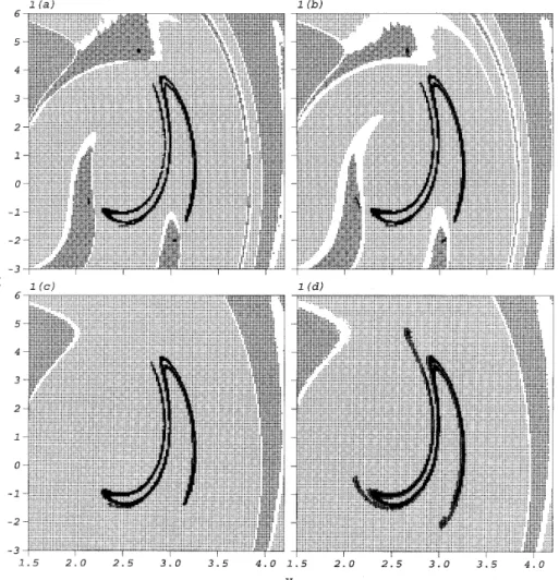
each cell to consider the effect of the random excitation, as in reference [15]. The attractors and basins of attraction located by GCM at varioussware shown in Figure 1. It is found
that as the noise level increases, the transient groups of multiple domicile cells and the persistent groups become larger. The periodic attractor of the corresponding deterministic system is destroyed by the noise at sw= 0·02. The two attractors of the corresponding
deterministic system are then combined into a large attractor by the noise at sw= 0·05.
Evolution of these results is physically reasonable. However, further study is necessary to determine the correctness of analysis using GCM.
As mentioned previously, GCM is applied to global analysis of random systems since it is more computationally efficient than Monte Carlo simulation. However, the number of sample records necessary to obtain reliable response statistics by Monte Carlo
simulation is of the order of 500. It is doubtful therefore that only ten sample functions can reflect the effect of the random excitation efficiently. Accuracy of analysis should not be sacrificed for the sake of computational efficiency, so we check the previous analysis by applying more sample functions to each cell. Moreover, a stable numerical method obtains consistent results when different parameter values are used in analysis, so we also vary the number of cells used for the identical region of interest. Some analyses for
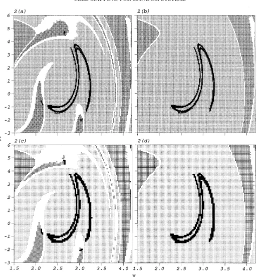
sw= 0·008 are shown in Figure 2. When the region of interest is divided into either 1512
or 1012cells, only one attractor in the region of interest is located by GCM as 20 sample
functions applied to each sampling point, but two attractors are located as 15 sample functions applied. Additionally, the located basins of attraction are very different in these analyses, as shown in Figure 2.
This inconsistency raises the question of which result is the most precise. Although the existing literature pays little attention to the correctness of global analysis, by using GCM, it is interesting to study the source of inconsistency among these results. It is found that
Figure 1. The attractors and basins of attraction of the Duffing oscillator, equation (1), located by GCM at various strengths of the random excitation: (a)sw= 0; (b)sw= 0·008; (c)sw= 0·02; (d)sw= 0·05. The symbol
‘‘+’’ denotes the basin of attraction of the sink cell, ‘‘×’’ and ‘‘·’’ for those of other attractors. Blank areas denotes the boundary regions, and black cubes the persistent groups.
Figure 2. The attractors and basins of attraction of the Duffing oscillator, equation (1), located by GCM at
sw= 0·008 for different numbers of cells and of sample functions of the random excitation applied to each
sampling point: (a,b) 1512cells, 15 and 20 sample functions; (c,d) 1012cells, 15 and 20 sample functions. The
symbols have the same meanings as in Figure 1.
this inconsistency should be due to the location of persistent groups based on various numbers of sample first mappings of cells. If more sample functions of the random excitation are applied to a set of cells that form a persistent group, the set may be expanded into a larger set of cells that still include all their sample first mappings. Otherwise, the corresponding attractor is destroyed by the random excitation. This condition of location of persistent groups is reasonable and conforms to analysis by Monte Carlo simulation, since the external loadings include a random excitation. However, the sample first mappings of cells are just the mappings of sampling points through one period. Thus, almost all of them are only transient mappings and cannot indicate the actual positions of attractors. Locating persistent groups in such a manner conflicts with the concept that an attractor is the stable motion of initial conditions over long enough periods. It overestimates the regions of the attractors located by GCM. Additionally, GCM uses multiple sampling points to represent a cell. If a sample first mapping of a sampling point of a cell in a persistent group reaches another cell, the reached cell must be included in
the persistent group to enable GCM to locate the corresponding attractor, and so must all image cells of the reached cell. This further overestimates the regions of the attractors located by GCM. An attractor is then not located if a sample first mapping of the corresponding persistent group reaches a multiple domicile boundary cell, even near the edge. However, the region of multiple domicile cells located by GCM is also much larger than the actual uncertain region of the system because of the latter two reasons. Thus, locating persistent groups by sample first mappings of cells makes difficulties in locating the attractors by GCM, for both deterministic and random dynamical systems.
Increasing the cell size then has more difficulty in locating persistent groups and is apt to make the attractor with a small basin of attraction not to be located in anlaysis for this system. Global analysis by GCM is then stopped since it leads to the false conclusion that this system has a single attractor in the region of interest and requires no further analysis. Moreover, the missing attractor will never be found after analysis, since global analysis by GCM is based on the persistent groups located and the result provides no information on the missing attractor. Decreasing the cell size by using more cells can of course improve the accuracy of analysis; however, the computational effort and memory required will severely limit application. These considerations imply that successful application of GCM to global analysis of a system is based on assigning an appropriate cell size. However, there is no easy way to assign an appropriate cell size in the region of interest unless all attractors have been located by other methods previously. These shortcomings of GCM can be remedied by using ICM instead. When applied to analysis of deterministic systems, ICM locates the attractors of initial conditions by the final mappings in the interpolated mapping sequences. ICM also defines a ‘‘strange attractor’’ as the attractor of all the initial conditions not attracted by the periodic attractors located. If there are missing attractors, this strange attractor provides information on them. These merits of ICM motivate us to develop a procedure using ICM for global analysis of random systems.
3. GLOBAL ANALYSIS OF RANDOM DYNAMICAL SYSTEMS BY ICM
The procedure of using ICM for global analysis of deterministic dynamical systems was stated in detail in references [7, 8]. The procedure is modified here, and the technique of Monte Carlo simulation included, for global analysis of random dynamical systems. In order to simplify development, the proposed procedure is applied only to analysis of systems forced by an ergodic random excitation [19], and the procedure for analysis of the systems with uncertain parameters is described later in this section. This two-stage procedure assumes that all initial conditions in a cell eventually reach the attractor of the node (the center of the cell). Before the analysis, a large number of sample functions through one period are simulated according to the characteristics of the random excitation. These sample functions are successively and cyclically assembled into Nn sets, with each
including Nr sample functions; here Nn is the total number of nodes. In the first stage of
analysis, each set of Nr sample functions is first applied to the corresponding node to
construct the Nr sample reference mappings of the node by numerical integration. Each
cell then has initial Nr sample mapping sequences including the effect of the random
excitation. The Nrfirst elements are its sample reference mappings at the first period, and
other elements are its sample mappings at later periods, given by interpolation of the sample reference mappings of nodes in the same order.
Note that as ICM is applied to analysis of a system forced by an ergodic excitation of zero average, a procedure of simulating only Nrsample functions and applying them to
each node in the same order is inappropriate for the following reasons. The sample functions of the ergodic excitation have zero time averages only if the sampled times
approach infinity [19]. However, these sample functions are simulated over only one period and have non-zero averages. The sample reference mappings of all nodes in the same order are thus constructed by an identical deterministic force of non-zero average, and so are all sample mappings of nodes in the same order given by interpolation. This violates the condition of zero average. A large number of sample functions, simulated and assembled into Nnsets as stated above, can reduce the error of construction of the sample mappings
of nodes through interpolation.
When ICM is applied to global analysis of a deterministic system, the periodic attractors and their basins of attraction are first located by the assigned criterion from the mapping sequences of cells within the assigned periods [7]. The cells which are not in the basins of attraction of the located periodic attractors are all considered to be in the basin of attraction of a ‘‘strange attractor’’: that is, the set of the final mappings of these cells. This strange attractor is introduced merely to indicate the attractors not located by the assigned criterion. Unless the periodic attractors and their basins of attraction are first located in such a manner, different basins of attraction cannot be delineated, since ICM does not register the final mappings of cells and no further analyses of attractors and basins of attraction can be processed after constructing the mapping sequences of cells. If this strange attractor still includes multiple attractors, global analysis by ICM fails since it does not delineate these attractors and their basins of attraction.
When ICM is applied to global analysis of a random system, the sample mappings of a cell are samplings of a discrete valued and discrete parameter vector stochastic process [19]; that is, positions of sample mappings are discrete at discrete sampled times. In addition, attractors of random systems are indecomposable closed invariant sets [3], and primarily indicated by their vector mean values and standard deviations. As in analysis of deterministic systems using ICM, attractors with cyclically stable vector mean values and standard deviations, and their basins of attraction, must be first delineated. Thus, the sample mappings of all nodes are constructed by interpolation of sample reference mappings in iterated Np, typically ten, periods to locate the attractors with periods of less
than Npand their basins of attraction. Each node has Nrsample mappings, a vector mean
value, and a vector standard deviation at each of the current Npperiods. The following
criteria are used to locate these attractors and their basins of attraction due to the use of a finite number of sample mappings. If two vector mean values of the sample mappings of a cell at different periods are within 0·05 of the cell size and the two corresponding vector standard deviations differ by a factor of less than 0·1, an attractor is considered to have been located. If all sample mappings of a cell lead outside the region of interest, the cell is considered to be in the basin of attraction of the sink cell. Additionally, if all the sample
Npth mappings of a cell lead to the vector mean values of an attractor with distances of
less than either the corresponding vector standard deviations or half a cell size, the cell is considered to be in the basin of attraction of the attractor. If the sample Npth mappings
of a cell lead to more than one located attractor, the cell is considered to be a multiple attractor boundary cell. The cells meeting each of these three cases require no further study since their attractors have been located. If some sample Npth mappings of a cell are not
attracted by the located attractors, they are assigned to the sample first mappings and then iterated forwards to construct the following sample mapping sequences. Sample mappings of different cells are so constructed through various periods to locate the attractors.
The first stage of global analysis of a random system is finished when the number of sample mappings of cells attracted by the located attractors is not increased and other sample mappings are iterated forwards over 50 periods. Here the maximum number of periods, Npm, used to construct the interpolated sample mappings of nodes is registered
been located. Other sample mappings are assumed to be attracted by an ‘‘undetermined attractor’’. This undetermined attractor is the set of attractors that exist in the region of interest and are not located by the assigned criteria. After this preliminary analysis, a cell with only some sample final mappings leading to a located attractor or residing in the basin of attraction of a located attractor is considered as a multiple attractor boundary cell, since its other sample final mappings lead to the undetermined attractor. Note that a set of cells that includes only some sample final mappings does not correspond to a closed set; also, a set of cells that includes all sample final mappings is just a positively invariant set [3, 4]. The algorithm used by GCM to locate persistent groups [4] is here introduced to reduce the sets of cells in which the located attractors and the undetermined attractor reside to indecomposable closed invariant sets of attracting cells based on sample final mappings of cells. Each attractor eventually has a corresponding closed invariant set of attracting cells. This algorithm for locating the sets of attracting cells is notably unlike that for locating persistent groups by GCM, since it uses the sample final interpolated mappings of cells, whereas GCM uses the sample first exact mappings of cells. Then the attracting cells of all attractors located by ICM must be further examined by Monte Carlo simulation. If a set of attracting cells includes more than one attractor, of course this global analysis by ICM fails. However, the analysis can generally be improved by reducing the region of study according to the positions of attractors. The attracting cells of the attractors located by ICM thus provide information on the correctness of global analysis using ICM and on how to improve global analysis.
In the second stage of analysis, the attractors and basins of attraction previously located must be further examined by more sample functions according to the technique of Monte Carlo simulation. Each multiple attractor boundary cell located requires no further study, since its existing sample mappings lead to at least two attractors. The cells adjoining the located boundary cells are possible multiple attractor boundary cells since the located boundary cells are sensitive to the random excitation. Additionally, the attracting cells of attractors must be studied further to characterize the transitions of attractors caused by the random excitation. Additional sample functions of the random excitation are hence applied to these critical cells to construct the new sample reference mappings for these critical cells. Sample mappings of the critical cells are then constructed by interpolation over Npm periods, with those at the last period used to characterize the transitions of the
attractors and their basins of attraction. When more sample functions are applied, the regions of the located boundary and attracting cells will increase, and the regions of the basins of attraction will decrease. If a new sample final mapping of a cell in the basin of attraction of an attractor leads to another attractor, the cell becomes a boundary cell. Additionally, if a new sample final mapping of an attracting cell reaches a cell in the same basin of attraction, the cell reached is considered to be an attracting cell in the identical set of attracting cells. Otherwise, the set of attracting cells is not a closed set of cells to meet the necessary condition for attractors. If a new sample final mapping of an attracting cell of an attractor reaches an attracting cell of another attractor, the former attractor is destroyed and all cells in its basin of attraction are considered to be attracted by the latter attractor. All boundary cells then need further analysis as before to locate their attractors. Global analysis of a random dynamical system by using ICM and Monte Carlo simulation is finished when the located boundary and attracting cells no longer change and each critical cell has been studied by at least fifty sample functions. The global analysis by ICM is finished here. The attractors, basins of attraction and boundary cells of the system are located.
Note that the boundary cells lead to at least two attractors with probabilities greater than zero and less than one. The final motions of these cells are therefore uncertain. On
the other hand, the cells in a basin of attraction are always attracted by only one attractor. This procedure is developed to locate the cells with definite final motions and those with uncertain final motions. Though this procedure is developed to study a system forced by a random excitation, it can be easily expanded to study systems forced by more than one random excitation. For analysis of the systems with uncertain parameters, samples of the uncertain parameters can be generated by numerous techniques [13]. Most of these techniques use random generators to produce independent realizations which are uniformly distributed over (0, 1). Random number generators are currently available in most computer software. The samples of uncertain parameters are then applied to construct the sample reference mappings of nodes by numerical integration. Other steps in the procedure are the same as those detailed above.
4. EXAMPLES OF APPLICATION
The method developed above is here applied to global analysis of random systems with uncertainties in external loadings or system parameters. These analyses are then compared with analyses using Monte Carlo simulation as fully as possible.
4.1. 1
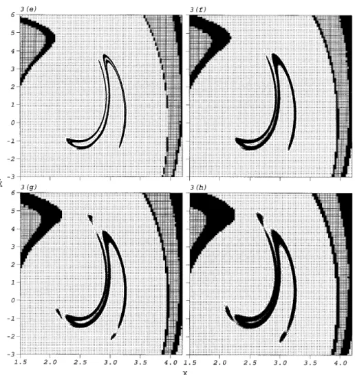
The proposed method is first applied to global analysis of the system governed by equation (1) at various strengths of the random excitation. The located attractors and basins of attraction for critical values of sw are shown in Figure 3. It can be seen that,
as the strength of the random excitation increases, the regions of attractors and of boundary cells become larger. The periodic attractor of the corresponding deterministic system is destroyed by the random excitation atswe 0·05. Then the two attractors of the
corresponding deterministic system are combined into a large attractor by the random excitation at swe 0·11. The evolution of these results is physically reasonable. At some
level of strength the random excitation may destroy the closeness of an attractor of the corresponding deterministic system; however, the attractiveness of the attractor due to the properties of the corresponding deterministic system always exists. For the attractor of period three at sw= 0·01, its vector mean values are (2·664, 4·663), (2·136, −0·622) and
(3·043, −2·000) located by ICM from the initial Nr sample mappings and (2·663, 4·676),
(2·133, −0·604) and (3·041, −2·004) located by Monte Carlo simulation; its vector standard deviations are (0·001, 0·009), (0·002, 0·012) and (0·002, 0·007) located by ICM and (0·002, 0·010), (0·002, 0·012) and (0·002, 0·008) located by Monte Carlo simulation. These results show good agreement.
Global analyses of this system by ICM require computational times ranging from one to three hours at various values of sw, based on the region of interest divided into 1012
cells, and Nr= 20 sample mappings constructed once for each cell and all critical cells. The
highest number of sample functions applied to the critical cells at various values ofswrange
from 540 to 1560. The computational times required for global analyses by GCM in section 2 range also from one to three hours, depending on the numbers of cells used and of sample functions applied to each sampling point. Some computational times required for analyses using ICM and GCM are listed in Table 1, based on computations performed on an IRIS Indigo workstation with 16 MB main memory. Generally, the global analysis by GCM with more sample functions applied to each sampling point requires more computational time but does not ensure more precise analysis. Despite the accuracy of the analysis, the computational times required for analyses by ICM and GCM are of the same order.
However, the highest number of sample mappings used by ICM is much greater than that used by GCM, since ICM constructs more sample mappings only for critical cells, and GCM constructs a uniform number of sample mappings for all sampling points of cells. In addition, the computational time required for global analysis by Monte Carlo simulation at each value of sw is at least 33 days according to the estimate of the time
necessary to construct all 1000 sample mappings for 1012initial conditions over 100 periods
by numerical integration. It is thus possible to examine only the transitions of attractors at various values of sw by Monte Carlo simulation.
Two initial conditions used, (2·66, 4·68) and (2·95, 1·50), are situated near the periodic attractor and strange attractor of the corresponding deterministic system. For a strength of the random excitation, if a sample mapping of the first initial condition leads to the region of the strange attractor of the corresponding deterministic system, the periodic attractor of the corresponding deterministic system is destroyed by the random excitation. If a sample mapping of the second initial condition leads to the region of the periodic attractor of the corresponding deterministic system, the two attractors of the corresponding deterministic system are combined into a large attractor by the random
Figure 3. The attractors and basins of attraction of the Duffing oscillator, equation (1), located by ICM at various strengths of the random excitation: (a) sw= 0·01; (b) sw= 0·02; (c) sw= 0·03; (d) sw= 0·04; (e)sw= 0·05; (f)sw= 0·10; (g)sw= 0·11; (h)sw= 0·16. The meanings of symbols ‘‘+’’, ‘‘×’’ and
‘‘·’’ are the same as in Figures 1 and 2. Black cubes denote the boundary cells, and small dots the attractors.
excitation. The sample mappings of these two initial conditions for the critical values of
sware shown in Figure 4, in which large dots denote the initial conditions used and small
dots the 500 sample mappings within the range of 50 and 500 periods. Figure 4(a) shows the sample mappings of these two initial conditions atsw= 0·04 and indicates that
there are still two attractors. Figure 4(b) shows the sample mappings of the first initial condition at sw= 0·05 and indicates that the periodic attractor of the corresponding
deterministic system is destroyed by the random excitation. Figure 4(c) shows the sample mappings of the second initial condition forsw= 0·09 and indicates that there is still only
one attractor. Figure 4(d) shows the sample mappings of the second initial condition at
sw= 0·10 and implies that two attractors of the corresponding deterministic system are
combined into a large attractor by the random excitation. The transition of the attractors studied by ICM is in good agreement with that studied by Monte Carlo simulation for this example.
4.2. 2
The proposed method is now applied to study global behaviour of a dynamical system with an uncertain system parameter. Consider a van der Pol oscillator governed by
x¨+z(x2− 1)x˙ + x = 0, (3)
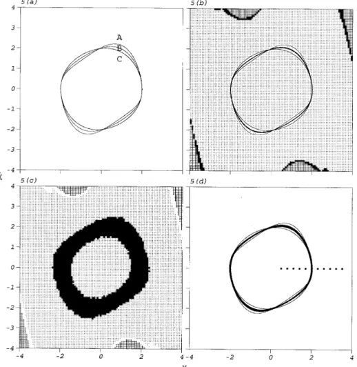
wherez is an uncertain parameter uniformly distributed over [0·1, 0·5]. For the fixed values of z, 0·1, 0·3 and 0·5, the attractors are the limit cycles shown in Figure 5(a), in which the curves A, B and C indicate the limit cycles forz = 0·5, z = 0·3 and z = 0·1 respectively. The uncertainty of this system thus raises a question as to what the attractor of this system is. Intuition may lead us to predict the attractor should wander between the two limit cycles for z = 0·1 and z = 0·5. ICM is applied to global analysis of the system with the region of interest (−4, 4) × (−4, 4) divide into 1012cells, and N
r= 20. Each sample mapping is
constructed over 0·01 × 50 = 0·5 time units. The only attractor located, compared with the three limit cycles in Figure 5(a), is shown in Figure 5(b). It is found that the attractor wanders about the limit cycle for z = 0·3. The result of global analysis by GCM is also shown in Figure 5(c) with 1012 cells and ten sample mappings applied to each of 32
sampling points of each cell. The located persistent group occupies a large region including the three limit cycles shown in Figure 5(a). The accuracies of analyses by ICM and GCM are then examined by Monte Carlo simulation. In Figure 5(d), large dots denote the initial conditions used and small dots the scope for the attractor located by Monte carlo simulation. It is found that the attractor wanders about the limit cycle of z = 0·3 as predicted by ICM. ICM hence obtains more precise analysis than GCM for this example. Additionally, the computational time required for analysis using ICM is 25 minutes with a maximum of 460 sample mappings constructed and that required for analysis using GCM is 35 minutes.
4.3. 3
To demonstrate how global analysis can be improved, ICM is applied to global analysis of a Duffing oscillator governed by the equation
x¨+ 0·1x˙ + x + x3= cos (2·5t) + w(t), (4)
T 1
Computational times required for various analyses of the system governed by equation (1)
Sampling Sample Maximum sample Time
Method sw Cells points mappings mappings (minutes)
GCM 0·008 1012 32 15 15 23 GCM 0·008 1012 32 20 20 70 GCM 0·008 1512 32 15 15 116 GCM 0·008 1512 32 20 20 158 ICM 0·01 1012 20 580 103 ICM 0·02 1012 20 700 121 ICM 0·03 1012 20 1140 182 ICM 0·04 1012 20 1140 181 ICM 0·05 1012 20 520 56 ICM 0·10 1012 20 980 130 ICM 0·11 1012 20 660 133 ICM 0·16 1012 20 860 85
Figure 4. At various strengths of the random excitation, the 500 sample mappings of the used initial conditions from 50 to 500 periods simulated by Monte Carlo simulation: (a)sw= 0·04, (2·66,4·68) and (2.95,1·50); (b) sw= 0·05, (2·66,4·68); (c) sw= 0·09, (2·95,1·50); (d)sw= 0·10, (2·95,1·50).
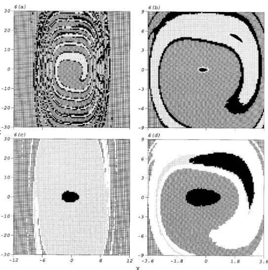
where w(t) is Gaussian and satisfies the conditions stated by equation (2). To tentatively characterize global behaviour of this system by ICM for sw= 0·28, the large region of
study (−12, 12) × (−30, 30) is divided into 1012cells, with N
r= 20. The numbers of cells
used by ICM and GCM are all the same for this example. Two attractors and their basins of attraction are located by this preliminary analysis, as shown in Figure 6(a). The attractors are situated around (−0·204, 0·016) and (1·784, 5·184). In order to study the detailed structure of the region surrounding these attractors, the region of study is reduced to (−3·6, 3·6) × (−9, 9). The attractors, basins of attraction and boundary cells are located as shown in Figure 6(b). In comparison with Figure 6(a), it is found that the cells in the basin of attraction of the sink cell do not lead to a new attractor. Hence, detailed study of the region surrounding the attractors is finished.
This reduction of the region of study is often used in practical engineering analyses. It is also applied to global analysis by GCM with ten sample mappings applied to each of 32sampling points of each cell. In Figure 6(c) is shown the single located attractor, near
may be stopped here since only one attractor is located in this region of study. However, a missing attractor is located by ICM even atsw= 0·92. GCM then locates two attractors
and their basins of attraction in the region (−3·6, 3·6) × (−9, 9), as shown in Figure 6(d). These two attractors occupy large regions. These analyses indicate that ICM allows one to improve global analysis on the basis of the result from a preliminary analysis more easily than GCM does. For the region of study, (−3·6, 3·6) × (−9, 9), the computational time required for analysis by ICM is 76 minutes, with a maximum of 1060 sample functions applied to the critical cells, and that required for analysis by GCM is 36 minutes.
5. CONCLUDING REMARKS
A method of using ICM for global analysis of random systems has been described. The development of the method was based on our study of inconsistent global analyses of the same system by GCM and on our study of the differences between ICM and GCM. When
Figure 5. The attractors and basins of attraction of the van der Pol oscillator, equation (3), located by different methods for differentz: (a) fixed z, by using numerical integration; (b) random z, by using ICM; (c) random
z, by using GCM; (d) random z, by using Monte Carlo simulation. The meanings of symbols in the analyses
Figure 6. The attractors and basins of attraction of the Duffing oscillator, equation (4), in different regions of study located by different methods: (a,b) (−12,12) × (−30,30) and (−3·6,3·6) × (−9,9), by using ICM; (c,d) (−12,12) × (−30,30) and (−3·6,3·6) × (−9,9), by using GCM. The meanings of symbols in the analyses by using GCM and ICM are the same as in Figures 1 and 3.
applied to study non-linear systems with uncertain external loadings or system parameters, the proposed method gives a more precise global analysis than GCM while requiring the same order of computational time. Global analyses by the proposed method agree well with those using Monte Carlo simulation. Additionally, the proposed method provides an easier way to improve a global analysis than GCM when the initial region of study is too large to have a precise global analysis.
ACKNOWLEDGMENTS
The authors wish to thank the referees for their valuable and helpful comments on this paper. These comments make the proposed method more complete and more definite. The authors are also grateful to the National Science Council, Republic of China, for support of this research under grant NSC 83-0401-E-009-078.
REFERENCES
1. J. M. T. T and H. B. S 1986 Nonlinear Dynamics and Chaos: Geometric Method for Engineers and Scientists. Chichester: John Wiley.
2. S. F and J. M. T. T 1991 Computer Methods in Applied Mechanics and Engineering 89, 381–394. Geometrical concepts and computational techniques of nonlinear dynamics. 3. J. G and P. H 1983 Nonlinear Oscillations, Dynamical Systems, and
Bifurcations of Vector Fields. New York: Springer-Verlag.
4. C. S. H 1987 Cell-to-cell Mapping: A Method of Global Analysis for Nonlinear Systems. New York: Springer-Verlag.
5. C. S. H 1992 International Journal of Bifurcation and Chaos 2, 727–771. Global analysis by cell mapping.
6. C. S. H and H. M. C 1986 Transactions of the American Society of Mechanical Engineers, Journal of Applied Mechanics 53, 695–701. A cell mapping method for nonlinear deterministic and stochastic systems—part I: the method of analysis.
7. B. H. T and K. G 1988 Transactions of the American Society of Mechanical Engineers, Journal of Applied Mechanics 55, 461–466. Interpolated cell mapping of dynamical systems. 8. B. H. T 1987 Physica D 28, 401–408. On obtaining global nonlinear system characteristics
through interpolated cell mapping.
9. W. K. L and M. R. G 1994 Transactions of the American Society of Mechanical Engineers, Journal of Applied Mechanics 61, 144–151. Domains of attraction of a forced beam by interpolated mapping.
10. J. A. W. S, C.A.L. D H, A. D and D. H. V C 1994 Nonlinear Dynamics 6, 87–99. Application of cell mapping method to a discontinuous dynamic system. 11. D. C and S. R. B 1994 Dynamics and Stability of Systems 9, 123–143. Periodic
oscillations and attracting basins for a parametrically excited pendulum.
12. M. S. S and J. M. T. T 1990 Dynamics and Stability of Systems 5, 281–298. Stochastic penetration of smooth and fractal basin boundaries under noise excitation. 13. R. Y. R 1981 Simulation and the Monte Carlo Method. New York: John Wiley. 14. S. H. C and W. Q. Z 1983 Transactions of the American Society of Mechanical
Engineers, Journal of Applied Mechanics 50, 953–962. Random vibration: a survey of recent developments.
15. J. Q. S and C. S. H 1991 Journal of Sound and Vibration 147, 185–201. Effects of small uncertainties on non-linear systems studied by the generalized cell mapping method.
16. J. B. R and P. D. S 1990 Random Vibration and Statistical Linearization. Chichester: John Wiley.
17. H. M. C and C. S. H 1986 Transactions of the American Society of Mechanical Engineers, Journal of Applied Mechanics 53, 702–710. A cell mapping method for nonlinear deterministic and stochastic systems—part II: examples of application.
18. C. S. H and H. M. C 1987 Journal of Sound and Vibration 114, 203–218. Global analysis of a system with multiple responses including a strange attractor.
19. T. T. S and M. G 1993 Random Vibration of Mechanical and Structural Systems. Englewood Cliffs, NJ: Prentice-Hall.
20. M. S and C.-M. J 1972 Journal of Sound and Vibration 25, 111–128. Digital simulation of random processes and its applications.