A BACKTRACKING METHOD FOR CONSTRUCTING PERFECT HASH FUNCTIONS FROM A SET OF MAPPING FUNCTIONS

BIT 25 (1985), 148-164

A B A C K T R A C K I N G M E T H O D F O R C O N S T R U C T I N G

P E R F E C T HASH F U N C T I O N S F R O M A SET OF

M A P P I N G F U N C T I O N S

Institute of Computer Engineering, National Chiao Tung University, 45 Po Ai Street, Hsinchu, Taiwan, Republic of China

Abstract.

This paper presents a backtracking method for constructing perfect hash functions from a given set of mapping functions. A hash indicator table is employed in the composition. By the nature of backtracking, the method can always find a perfect hash function when such a function does exist according to the composing scheme. Simulation results show that the probability of getting a perfect hash function by the backtracking method is much higher than by the single-pass and multipass methods previously proposed.

1. Introduction.

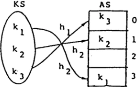
Hashing is a widely used technique for information storage and retrieval [11, 12, 13, 14, 15]. A one-to-one correspondence hash function from key space to address space is called a perfect hash function. Many approaches have been proposed for constructing perfect hash functions [1, 3, 4, 5, 6, 9, 10, 16, 17]. Recently, Du, Hsieh, Jea and Shieh [6] proposed a perfect hash scheme in which rehashing and segmentation have been employed in constructing hash functions. Rehash means to solve the key collision problem by using a series of hash functions, h 1, h2, ...,h s. Segmentation means to divide address space into segments before allocating them. A hash indicator table (HIT) is used to store the index of hash functions. A hash function h can be defined by HIT as follows

[6]:

h(k,)

xi

HITChr(ki), ] 4= r

HIT[hj{ki) ] = j,

= undefined, otherwise.

When h is defined on all keys concerned, it is a perfect hash function.

The advantages of the perfect hash functions defined by H I T here are: they

A BACKTRACKING METHOD FOR CONSTRUCTING PERFECT HASH . . . 149

are easy to implement a n d they use only small tables. T w o ways for c o n s t r u c t i n g H I T have been p r o p o s e d in I-6, 17]. We shall discuss t h e m briefly in Section 2.2. In Section 3, we introduce a n o t h e r m e t h o d to c o n s t r u c t H I T which is based on a b a c k t r a c k i n g technique. We present the a l g o r i t h m o f this scheme a n d discuss its efficiency. In Section 4, we study the probability of getting a perfect hash function by this m e t h o d in c o m p a r i s o n with the other two methods.

2. Construction o f a H I T .

2.1 The Problem

Consider the matrix of Figure 1. There are three keys, kl,

k2,

kl kz k3

h I 2 2 0

h 2 3 1 1

Fig. 1. A 2 x 3 mapping table.

hash functions, hi, a n d hz ; i.e., we have key space K S = {kl,

k2, k3}

space AS = {0, 1, 2, 3}. T h e matrix is called a m a p p i n g table. T h e p r o b l e m here is to c o n s t r u c t a perfect hash function h which is c o m p o s e d o f h I a n d h 2. F o r example, one h is defined as follows:

f h E ( k l ) = 3;

h(ki) = h~(ki) = ~hE(k2) 1 ;

I.hl(k3) 0.

T h e perfect hash function h c a n be expressed as Figure 2 o r Figure 3.

K S A S

h

1

2 3

150 W . P . YANG AND M. W. DU K S l l , h 2 I !

2/

:

I

Fig. 3. A perfect hash function h is composed of h 1 and h 2 and HIT is used.

In Figure 3, we use H I T to store the index of the hash functions h I and h 2. This table stores the information of whatever function is used to compute the address of the keys in KS. For example, hi(k3) = 0 and HIT[0] = 1, imply that the key k 3 stored in the AS[0] at address 0 is computed by using h r This rule applies to the other entries of HIT. Since only the indices of hash functions are stored, the width of a HIT can be made small. When H I T is stored in the main memory, only one disc access is needed to retrieve a record. The retrieval algorithm is quite simple as proposed in [6, 17]. We list it below:

Procedure RETRIEVAL(k, s, HIT, AS);

/ / Assume that the hash functions hi, h2, / /

/ / . . . . h s, are used to create the HIT. / /

/ / Now we want to retrieve key k. / /

begin

j : = l ;

while (HIT[h~(k)] ~ j a n d j < s) d o j : = j + 1; i f j > s then failure

else k is stored in AS[h~(k)] end.

In evaluating the function value, the number of loops executed in the statement in the algorithm is called the "number of internal probes" in HIT. 1 ~ ' - I HIT[i], where n is the number of keys Retrieval cost is defined by n - z_,i=0

concerned and r is the size of the address space. The optimal solution is the one among all feasible solutions with the smallest retrieval cost. For a given mapping table, the problem is how to construct a H I T which defines a perfect hash function.

2.2 Previous work on constructiny H I T

The H I T construction problem was first studied in [6] which proposed a procedure called multi-pass method and then in [17] with another procedure called single-pass method. In the following we explain the operations of these two procedures briefly by applying them to Figure 1 of Section 2.1.

A BACKTRACKING METHOD FOR CONSTRUCTING PERFECT HASH . . . 151

M e t h o d 1" Multi-pass procedure

(1) Select all the singletons from the first row, such as 0 in the following table. An entry in row h and column k is a singleton if there is no other k' such that

h(k') = h(k).

(2) Select all the singletons from the second row except from those columns which have been selected in the first row, such as 3 and 1 in the following table. We then accomplish and obtain a perfect hash function with HIT = (1, 2,0, 2).

krt k2 k3 . . . 2 2 (~) hi

O

O

1

(Basically, we will process the keys in the order k 1, k2, etc.) (1) We process k 1 and circle 2.

kl k2 k3

hi @ 2 0

h 2 3 1 1

. . .

(2) We process k2. Note that k2 has the same hash value as kl by applying h r In this case, kl and k 2 collide and both need rehashing by h 2. Thus we get the following result :

kt kz k3

hi 2 2 0

®

O

1

(3) Finally, we process k 3. Since zero is a singleton in the first row, we circle it and obtain a perfect hash function with HIT = (1, 2, 0, 2).

kl k2 ka

. . .

h I 2 2 @

®

O

1

From the discussion above, the main difference between the multi-pass and single-pass approaches is the way to select singletons. While multi-pass

152 W. P. YANG AND M. W. DU

approach would select singletons row by row, single-pass approach would process the keys column by column. The two schemes may have different results. So for a given mapping table it is possible to get a perfect hash function by a multi-pass method but it would be a failure by a single-pass method and vice versa.

EXAMPLE 1. [Failure for multi-pass; success for single-pass method]

Let the key set be KS = {k 1, k2, k 3, k4}. The address space has a size of five

entries. The three hash functions are defined by the following table:

h 1 h2 h3 kl k2 k3 k4 . . . 2 3 2 3 3 t t 0 4 2 3 1

(1) By applying the multi-pass procedure, we have:

3 0

- 2

That is, the key k3 cannot be placed in address space, therefore the hash function is not perfect.

(2) By applying the single-pass procedure, we have:

0 4 2 3 -

That is, the hash function h is perfect and defined by HIT = (2, 0, 3, 3, 3). EXAMPLE 2 [Success for multi-pass; failure for single-pass method]

In the following mapping table:

kl k2 k3 k 4

h I 4 3 3 4

h z 1 4 2 3

......................................

A B A C K T R A C K I N G M E T H O D F O R C O N S T R U C T I N G P E R F E C T H A S H . . . are as follows:

1 4 2 3 1 - 2 3

(success for multi-pass) (failure for single-pass)

EXAMPLE 3 [Failure for both multi-pass and single-pass methods] Consider the following mapping table:

k l k2 k3 k3 . . . h 1 3 4 2 4 . . . h I 4 3 2 1 153

The HIT constructed by the multi-pass and the single-pass methods are both (0, 2, 1, 1, 0), or

3 - - 2 - - 1

Therefore it does not define a perfect hash function.

In Example 3, however, we can find two perfect hash functions as defined by HIT = (0, 2, 1, 2, 2) and HIT = (0, 2, 2, 2, 2). I.e.,

2 . . . . .

and

4 3 - 1 4 3 2 1

In the following we will introduce a backtracking method to find (1) all the feasible solutions, (2) the optimal solution (i.e., with the lowest retrieval cost), and (3) an answer of "no solution" if no solution exists, according to a given mapping table.

3. Algorithm and efficiency.

3.1 Basic concepts

In applying a backtracking technique finding the "intelligent" bounding function is important. Different problems (for example, the 8-queens problem, sum of subsets, graph colouring, Hamiltonian cycle and knapsack problems [2, 7, 8]) have different bounding functions. Given a mapping table, our problem is to construct a HIT to define a perfect hash function. Thus the goals of our bounding function are: (1) Each key in the key space corresponds to a unique address in the address space, and (2) The retrieval algorithm should work correctly. Assume that the solution is (xl, x2 ... x,), where xi are chosen from

154 W . P. Y A N G A N D M. W . D U

c o l u m n i in the m a p p i n g table. The first of these two goals implies that no two x~ can be the same. T h a t is:

(a)

Assume i ~ j and x i = hz(kj), x i = hv(ki), then the second goal is: (see Figure 4)

(b)

hip..

Q

©

Suppose that ( x l , x2 . . . x,,) is a solution which satisfies the constraints (a) and (b), where x i = ht,(ki) for key k i and some hash function h 6. Then the H I T c o r r e s p o n d i n g to this solution can be constructed by letting

HIT[ht,(k3] = I i for each i < n.

T o simplify the explanation, we will consider a problem of constructing a perfect hash function on a 2 x 3 matrix• Figure 5 shows the configurations as the backtracking proceeds.

®

2

@

@

®

l

1

®

®

l

®

®

1

A BACKTRACKING METHOD FOR CONSTRUCTING PERFECT HASH . . . 1 5 5

The problem is that exactly one value must be selected in each column. In the beginning a value is selected in the first column of the first row, at position (1,1), as shown in Figure 5(a), indicated by a circle. Here we have (X1, X2,'X3) = ( 2 , - , - ) . The next value is selected from position (1, 2), (xl,xE,x3) = (2,2,-), as shown in Figure 5(b). Since no two x i can be the same, it is necessary to reconsider the first column and select the value at position (2, 1), (xl,Xz, X 3 ) - - ( 3 , - , - ) , as shown in Figure 5(c). Note that we need not check the states of (2,2,0) and (2,2, 1). In Figure 5(d), the value 2 at position (1, 2) is the same as the value at position (1, 1). This selection will make future retrieval operations fail, so we discard this value, and select the value 1 at position (2,2), as shown in Figure 5(e). Finally, the value 0 in column 3 at position (1, 3) is selected, and we get a feasible solution, as shown in Figure 5(f); i.e., we constructed a perfect hash function with H I T - - ( 1 , 2 , 0 , 2 ) . The backtracking algorithm determines problem solutions by systematically searching the solution space for the given problem instance. This search is simplified by using a tree organization for the solution space. In the example the backtracking traverses the nodes of the tree as shown in Figure 6 along the dotted arrows.

xl.hl ( i I -3

x2"hZ(k2)'2

Fig. 6.

)

The depth first order in which backtracking examines the tree o f solution space is shown by the dotted arrows.

3.2 Algorithm

Here we define s o m e terminological concepts regarding tree organization of solution spaces (see Figure 6). Each node in the tree defines a problem state. All paths from the root to other nodes define the state space of the problem. Solution states are those problem states S for which the path from the root to S defines a tuple in the solution space. In the tree of Figure 6, only the leaf nodes are solution states. Answer states or feasible solutions are those solution states S for which the path from the root to S defines a tuple which is an element of the set of solutions (i.e., it satisfies the constraints) of the problem. The tree

156 W, P. YANG AND M. W. DU

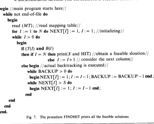
organization of the solution space will be referred to as the state space tree. Given a mapping table MT, the procedure "FINDHIT" prints all the feasible solutions which define perfect hash functions by using backtracking techniques. The procedure is listed in Figure 7. The variables used are defined as follows: N R S I M T X INDEX NEXT BACKUP

number of the key set. size of the address space. number of rehash functions.

index of the value in the solution vector. mapping table.

solution vector.

contains row numbers for the corresponding x-values in the mapping table (i.e. the index of hash functions).

NEXT(i) points to the next row to be tried in column i. is the number of columns to go back in the problem states.

PROCEDURE FINDHIT;

Var MT: array[1... S, 1... N] of integer;

X, INDEX, NEXT: array[1... N] of integer;

HIT: array[1 ...R] of integer;

L K, BACKUP: integer;

FUNCTION T(/): boolean;//generating the next problem states//

begin T := false; if NEXT[/] < S then

begin INDEX[/] := NEXT[/] ; X[/] := M T [ I N D E X [ / ] , / ] ; NEXT[/] := NEXT[l] + 1 ; T := true end

end;

else end;

FUNCTION B(/): boolean;//bounding function// begin B := true;

for K : = 1 t o I - l d o if X[K] = X[/]

then begin B := false;//violate constraint(a)//

if INDEX[K] = INDEX[l] //with same hash function//

then if INDEX[K] = 1 //h 1 is used in the first row//

then B A C K U P : = l - K / / b a c k t r a c k k - i columns//

else BACKUP := 1 //backtrack to previous column/

end

if (NEXT[K] > NEXT[/]) and (MT[INDEX[/], K] = X[/])

A B A C K T R A C K I N G M E T H O D F O R C O N S T R U C T I N G P E R F E C T H A S H . . . 1 5 7

b e g i n / / m a i n p r o g r a m starts h e r e / / while not end-of-file do

begin read ( M T ) ; / / r e a d m a p p i n g t a b l e / / for I : = 1 t o N do N E X T [ / ] : = l, I : = 1 ; / / i n i t i a l i z i n g / / while I > 0 flo begin if (T(/) and B(I)

then if I = N then print(X and H I T ) / / o b t a i n a feasible sloution// else I : = I + 1 / / c o n s i d e r the next column//

else b e g i n / / a c t u a l backtracking is executed// while B A C K U P > 0 do begin N E X T [ / ] : = 1 ; I : = I - 1 ; B A C K U P : = B A C K U P - 1 end ; while N E X T [ / ] > S do begin N E X T [ / ] : = 1 ; I : = I - 1 end; end end end end.

Fig. 7. The procedure F1NDHIT prints all the feasible solutions.

Generating the next problem state, T

The boolean function T(i) is used to test whether (xl,x2 ... x~) is in the

p r o b l e m state. If it is true, it implies that x~ is assigned from one value of column i in the M T , and (xl,x2 ... xi-~) have already been chosen. N o w the

solution vector is extended to i values, and xg (to be called the value of current state or current value in short) is considered as a component of a feasible solution. Bounding function, B

The bounding function B(i) is false for a path (Xl, x2 . . .

Xi)

cannot be extended to reach an answer node, i.e., the bounding function Bi returns a boolean value which is true if the ith x can be selected in the column i of the m a p p i n g rable M T , and can satisfy the constraints (a) and (b) in Section

3.1. Thus the candidates for position i of the solution vector X(1 ... n) are those values which are generated by T(i) and satisfy B(i). If i = n, we obtain a feasible

solution and then print it.

EXAMPLE 4 [Backtracking method to construct H I T ] Consider the following m a p p i n g table:

kl k2 k3 k4

1 1 2 1

3 0 2 4

hi h2

158 w . P . YANG AND M. W. DU

The size of the solution space is 16. By using the p r o c e d u r e F I N D H I T , t w o feasible solutions are o b t a i n e d as

2 . . .

a n d

3 0 - 4 3 0 2 4

with H I T = (2, 0, 1, 2, 2) and H I T = (2, 0, 2, 2, 2) respectiveiy. T h e first solution is the optimal with retrieval cost equal to 1.75.

EXAMPLE 5 [ B a c k t r a c k i n g one or m o r e steps] Consider the following m a p p i n g table:

h 1 h2 ha h4 k l k2 k3 k4 k5 k6 k 7 k s k 9 k l o . . . 4 2 5 6 4 3 8 12 4 12 6 5 12 3 4 13 3 5 6 5 . . . 5 15 3 6 7 5 6 4 3 I1 . . . 4 2 5 I1 4 3 17 16 4 . 14 . . .

By using the p r o c e d u r e F I N D H I T , the first four solutions can be easily obtained as shown in the Appendix. Before we find the first solution, we s h o u l d reach a problem state as shown in Figure 8(a). I n the figure the partial values

(circled) of the solution vector are X = (4, 2, 5, 6 . . . -), a n d the current

value is 4 (shown by a square box). Since X[1-] = X [ 5 ] = 4, it is impossible to have feasible solutions such that X [ 1 ] = 4 because the constraints (a) o r (b) would be violated. Therefore, it m u s t b a c k t r a c k the p r o b l e m state from I = 5 to I = 1 as shown in Figure 8(b). Figure 8(c) shows the fourth solution. In o r d e r to find the next solution, the following p r o b l e m states are generated and are tested. We show t h e m by Figures 8(d), 8(e), 8(f) and 8(g). I n Figure 8(g), again, we have X [ 1 ] = X [ 6 ] = 5. If we b a c k t r a c k 5 steps (backtrack to the first column), as shown in Figure 8(h), we m a y lose some feasible solutions. O n l y a one-step b a c k t r a c k i n g (backtrack to c o l u m n 5) is correct as s h o w n in Figure 8(i). Therefore, the solution o b t a i n e d in Figure 8(j) is o u r fifth feasible solution. Some other solutions are listed in the Appendix.

® @ @ @ []

6 5 12 3 4 13 3 5 6 5

5 15 3 6 7 5 6 '4 3 11

4 2 5 11 4 3 17 16 4 14

"11 .00 f~ Q GI ~ ~ ~ Z 0

160 w . P . YANG AND M. W. DU 4 2 5 6 4 3 8 12 4 12 6 5 12 3 4 13 3 5 6 5 5 15 3 6 7 5 6 4 3 11 5 15 3 6 7 5 6 4 3 11 [ ] 2 5 11 4 3 17 16 4 14 (h) 4 @ 5 @ 4 3 8 12 4 12 6 5 @ 3 4 13 3 5 6 5 @ 15 3 6 [ ] 5 6 4 3 11 4 2 5 I1 4 3 17 16 4 14 , (i) 4 @ 5 @ 4

@ @

Fig, 8. Behavior of the backtracking of Example 4.

3.3 Efficiency

How effective is the algorithm F I N D H I T over the brute force approach? For a 2 × 4 matrix as shown in Example 2, there are 31 nodes in the tree organization of the solution space. That is, there are 31 problem states. Some states are ignored by the constraints of the bounding function B. Hence we need to examine only 12 problem states. The efficiency of the algorithm is thus defined by :

efficiency = T1/ T 2,

where T 1 denotes the number of nodes generated by the backtracking algorithm, and T z denotes the number of nodes in the state space tree. In Example 2, the efficiency is only about 0.387. This implies that only 38.7 percent of the nodes need be examined in order to find the feasible solutions. Since the efficiency is data dependent, we design an experiment to estimate some average values of efficiency. Column (a) in Figure 9 shows the expected values of efficiency to find a feasible solution set. Column (b) shows the expected values of efficiency to find the optimal solution. For a given mapping table, if the perfect hash function does not exist, we say there is no solution. Using the backtracking algorithm, we can determine whether there is no solution by only generating the

A B A C K T R A C K I N G M E T H O D F O R C O N S T R U C T I N G P E R F E C T H A S H . . . 1 6 1

partial nodes (the number is denoted by T1) instead of testing all the nodes in the state space tree (T2). Column (c) shows the expected values of efficiency to find no solution. All the values are computed from the average of 100 independent test data sets, with loading factor (i.e., (size of KS)/(size of AS))

= 0 . 8 . ( a = 0 . 8 ; s = 3) k e y ( a ) ( b ) (c) n o . a f e a s i b l e o p t i m a l n o s o l u t i o n 5 0 . 0 7 4 4 0 . 2 3 1 2 0 . 1 5 6 7 10 0 . 0 0 4 2 0 . 0 2 4 6 0 . 0 0 9 3 . . . . . . 15 1.8 * 10 - 4 7 . 4 , 1 0 - 4 3.0 * l 0 - 4 20 7 . 4 * 10 - 6 2 . 6 * 10 - 5 6 . 7 * 10 - 6 F i g . 9. V a l u e s o f e f f i c i e n c y , 4. Comparison results.

Suppose the mapping tables have random hash values; i.e., the hash values in each mapping table are uniformly distributed over the range, Let P,,, Ps, and Pb denote the probability of getting perfect hash functions by using multi-pass,

Prob. ~.o~ O.gr 0.8i, O.7t 0.~1 O.S| 0.4~ 0.] 0o~ 0.] 0.01 I.o 15 " - 20 2 S -" 30 • - ] ; o - 0 . 6 • ' Pm m ~ t ~ l - o ~ s s ~ p $ s L ~ q L e - p a s s - - ' ~ - - P b back~ra~ ~'S " n p o o h .

,.ot

162 W. P. YANG AND M. W. DU

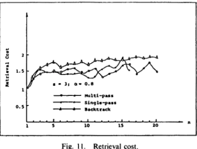
single-pass, and backtracking methods respectively. The procedures for the three methods were programmed in Pascal and their probabilities evaluated on a CDC Cyber 170/720 computer. The results of this evaluation are presented in Figure 10. As the figure indicates, the backtracking method is better than multi- pass and single-pass methods. The retrieval costs of the three methods are also presented in Figure 11. All of them are within a limit, not exceeding 1.95, in the case s = 3.

21

are listed in the Appendix.

Appendix. M A P P I N G T A B L E IS: 4 2 5 6 4 3 8 12 4 12 6 5 12 3 4 13 3 5 6 5 5 15 3 6 7 5 6 4 3 11 4 2 5 11 4 3 17 16 4 14 SIZE O F S O L U T I O N SPACE: 1048576

Fig. 1 I. Retrieval cost.

5. Conclusion.

This paper presents a backtracking method to construct perfect hash functions from a set of mapping functions. Compared with the other two methods proposed before, this new method has a much better chance to get perfect hash functions. For example, as n = 25, ct = 0.8, s = 7, the probability of getting a perfect hash function is around 97 %. The only problem is that when n increases, the probability of getting a perfect hash function decreases. But this difficulty can be overcome by segmentation, i.e., by dividing the address space into segments. This idea was first used in [6] and was also applied in [17].

If perfect hash functions do exist in a given mapping table, the backtracking method can certainly find all of them and give the optimal solution. It is surprising that, in a mapping table of dimensions 4 x 10, we get 204 feasible solutions, with efficiency of 0.006. The matrix and some of the feasible solutions

A B A C K T R A C K I N G M E T H O D F O R C O N S T R U C T I N G P E R F E C T H A S H . . . 163 F E A S I B L E S O L U T I O N : ( l ) - 2 - 6 8 1 2 - 4 13 - - - 5 . . . 3 l l . . . 16 H I T = ( 0 , 1 , 3 , 2 , 3 , 1 . . . . ) C O S T = 2 . 2 0 ( 2 ) - 2 - 6 - 8 12 - 4 13 . . . . 5 . . . 3 - . . . 16 - 1 4 H I T = (0, 1o 3, 2, 3, 1 . . . . ) C O S T = 2 . 3 0 3 ) - 2 - 6 - - 1 2 - 4 13 . . . . 5 . . . 3 11 17 16 H I T = (0, 1, 3, 2, 3, 1 . . . . ) C O S T = 2 . 5 0 ( 4 ) - 2 - 6 . . . 12 - 4 1 3 5 . . . 3 - . . . 1 7 16 - 1 4 H I T = (0, 1, 3, 2, 3, 1 . . . . ) C O S T = 2 . 6 0 ( 5 ) - 2 - 6 - 3 8 12 . . . . 5 7 . . . . 11 . . . 16 4 H I T = ( 0 , 1 , 1, 4 , 3 , 1 . . . . ) C O S T = 2 . 3 0 ( 6 ) - 2 - 6 - 3 8 1 2 - - 5 7 . . . 16 4 14 H I T = (0, 1, 1, 4, 3, 1 . . . . ) C O S T = 2 . 4 0 ( 7 ) - 2 - 6 - 3 12 - 5 7 . . . 11 . . . 1 7 16 4 - H I T = (0, t , 1, 4, 3 , 1 . . . . ) C O S T = 2 . 6 0 ( 8 ) - 2 - 6 - 3 t 2 . . . . 5 - - 7 1 7 16 4 1 4 H I T = (0, 1, 1, 4, 3, 1 . . . . ) C O S T = 2 . 7 0 ( 9 ) - 2 - 6 8 1 2 13 . . . . 5 7 4 3 11

164 w . P . YANG AND M. W. DU H I T = (0,1,3,3,3,1 . . . . ) C O S T = 2 . 2 0 ( 1 0 ) - 2 6 8 - - 12 13 5 7 4 3 . . . 14 HIT = (0, 1, 3, 3, 3, 1 .. . . ) COST = 2.30 O P T I M A L S O L U T I O N : ( 1) E F F I C I E N C Y = 0.006 = 8605/1398101 (204) . . . . 12 13 - - - 7 3 - 4 2 11 - 17 16 - 14 HIT = (0,4,3,4,0,0,...) COST = 3.00

Acknowledgement.

The authors wish to thank the a n o n y m o u s referee for his valuable and constructive comments.

R E F E R E N C E S

1. M. R. Anderson and M. G. Anderson, Comments on perfect hashing functions: A single probe retrieving method for static sets. Comm. A C M 22, 2 (Feb. 1979), 104.

2. J. R. Bitner and E. M. Reingold, Backtrack programming techniques. Comm. ACM 18, 11 (Nov. 1975), 651-656.

3. R. J. Chichelli, Minimal perfect hash functions made simple. Comm. A C M 23, 1 (Jan. 1980), 1%19.

4. C. R. Cook and R. R. Oldehoeft, A letter oriented minimal perfect hashing function. A C M Trans. on S I G N P L A N NOTICES 17, 9 (Sept. 1982), 18-27.

5. C. C. Chang, The stud),, of an ordered minimal perfect hashing scheme. Comm. A C M 27, 4 (April 1984), 384-387.

6. M. W. Du, T. M. Hsieh, K. F. Jea and D. W. Shieh, The study of a new perfect hash scheme. IEEE Trans. on Software Engineering, SE-9, 3 (May 1983), 305-313.

7. S. W. Goloma and L. D. Baumert, Backtrack programming. JACM 12, 4 (1965), 516-524. 8. E. Horowitz and S. Sahni, Fundamentals of Computer Algortthms. Computer Science Press,

INC., 1978.

9. G. Jaeschke and G. Osterburg, On Chiehelli's minimal perfect hash functions method. Comm. A C M 23, 12 (Dec. 1980), 728-729.

10. G. Jaeschke, Reciprocal hashing: A method for generating minimal perfect hashing functions. Comm. A C M 24, 12 (Dec. 1981), 829-833.

11. D. E. Knuth, The Art of" Computer Programming, Vol. 3, Sorting and Searching. Addison- Wesley, Reading, Mass., 1973.

12. W. D. Maurer, An improved hash code for scatter storage. Comm. A C M 11, 1 (Jan. 1968), 35-37.

13. W. D. Maurer and T. G. Lewis, Hash table method. Computing Surveys 7, 1 (Mar. 1975), 5-19. 14. R. Morris, Scatter storage techniques. Comm. A C M 11, 1 (Jan. t968), 38-44.

15. D. G. Severance, Identifier search mechanisms: A survey and generalized model. Computing Surveys 6, (Sep. 1974), 175-194.

16. R. Sprugnoli, Perfect hashing, functions: A single probe retrieving method for static sets. Comm. A C M 20, 11 (Nov. 1977), 841-850.

17. W, P. Yang, M. W. Du a n d J. C. Tsay, Single-pass perfect hashing for data storage and retrieval. Proc. 1983 Conf, on Information Sciences and Systems, Baltimore, Maryland, Mar.