Inverse Determinant Sums and Connections Between
Fading Channel Information Theory and Algebra
Roope Vehkalahti, Member, IEEE, Hsiao-Feng (Francis) Lu, Senior Member, IEEE, and Laura Luzzi, Member, IEEE
Abstract—This work considers inverse determinant sums, which arise from the union bound on the error probability, as a tool for designing and analyzing algebraic space-time block codes. A gen-eral framework to study these sums is established, and the con-nection between asymptotic growth of inverse determinant sums and the diversity-multiplexing gain tradeoff is investigated. It is proven that the growth of the inverse determinant sum of a divi-sion algebra-based space-time code is completely determined by the growth of the unit group. This reduces the inverse determi-nant sum analysis to studying certain asymptotic integrals in Lie groups. Using recent methods from ergodic theory, a complete clas-sification of the inverse determinant sums of the most well-known algebraic space-time codes is provided. The approach reveals an interesting and tight relation between diversity-multiplexing gain tradeoff and point counting in Lie groups.
Index Terms—Algebra, diversity-multiplexing gain tradeoff (DMT), division algebra, Lie groups, multiple-input mul-tiple-output (MIMO), number theory, space-time block codes (STBCs), unit group, Zeta functions.
I. INTRODUCTION
I
N this paper, we introduce a new technique to analyze the performance of lattice space-time block codes in the high SNR regime. By developing the analysis based on the union bound of the pairwise error probabilities of such codes, we show that the high-SNR performance is related to the asymptotic be-havior of the inverse determinant sums of these codes. The new performance criterion based on inverse determinant sums fills in the middle ground between the diversity-multiplexing tradeoff (DMT) [16] and the normalized minimum determinant.The normalized minimum determinant criterion has been used effectively to choose which space-time code one should Manuscript received November 27, 2011; revised December 23, 2012; ac-cepted April 02, 2013. Date of publication June 05, 2013; date of current ver-sion August 14, 2013. R. Vehkalahti was supported by the Academy of Finland under Grants 131745 252457. H. F. Lu was supported in part by the Taiwan National Science Council under Grants NSC 100-2221-E-009-046-MY3 and NSC 101-2923-E-009-001-MY3. L. Luzzi was supported in part by a Marie Curie Fellowship (FP7/2007-2013, Grant agreement PIEF-GA-2010-274765). This paper was presented in part at 2011 IEEE International Symposium on In-formation Theory, in part at the 2011 IEEE InIn-formation Theory Workshop, and in part at the 2012 IEEE International Symposium on Information Theory.
R. Vehkalahti is with the Department of Mathematics, University of Turku, Turku 20100, Finland (e-mail: [email protected]).
H.-F. (Francis) Lu is with the Department of Electrical Engineering, National Chiao Tung University, Hsinchu 300, Taiwan, R.O.C. (e-mail:francis@mail. nctu.edu.tw).
L. Luzzi is with Laboratoire ETIS, ENSEA–Université de Cergy-Pon-toise–CNRS, Cergy-Pontoise 95014, France (e-mail: [email protected]).
Communicated by J.-C. Belfiore, Associate Editor for Coding Theory. Digital Object Identifier 10.1109/TIT.2013.2266396
use in order to get the best performance. For a relatively high-SNR level this optimization has produced very good results. However, this criterion concentrates on minimizing the worst-case pairwise error probability, and does not consider its overall distribution, disregarding for example the question of how many times the worst-case scenario occurs.
The DMT, on the other hand takes into account the overall error probability, but only in the asymptotic sense as the SNR and codebook size grow to infinity. Moreover, the DMT focuses only on the diversity exponent, and in many cases it is too coarse for practical code design. For example, from the DMT point of view almost all full-rate division algebra-based codes are equiv-alent in terms of diversity exponent, while their actual perfor-mances often differ strongly.
The asymptotic growth of the inverse determinant sum cap-tures something between these two concepts. Our analysis re-veals that the diversity-multiplexing gain bounds of Zheng and Tse [16] constitute general lower bounds for the asymptotic growth of inverse determinant sums. The bounds depend on the dimension of the lattice and on the number of transmit and re-ceive antennas. Achieving such bounds immediately proves that a code is DMT optimal for multiplexing gains between , while in other cases the asymptotic growth provides informa-tion on the DMT for multiplexing gains in this region. Further-more, the behavior of inverse determinant sums can be analyzed with great accuracy and can provide information also on the nor-malized minimum determinant. But, in this paper we are mostly interested in the interplay between DMT and inverse determi-nant sums and will only consider exponents of the growth of the latter.
While the first part of the paper is about stating the problem and proving general lower bounds, the second part concentrates on analyzing the growth of inverse determinant sums of large classes of algebraic space-time codes. Most of the division al-gebra-based codes are subsets of an order [4] inside the division algebra. Using orders guarantees the nonvanishing determinant property (NVD), which has been shown to be a sufficient crite-rion for DMT optimality for lattice codes in the space having full rank [5] and [6].
We will prove that the growth of the inverse determinant sum of a division algebra-based space-time code depends only on the asymptotic growth of the norms of the unit group of the under-lying order, and can be computed from invariants of the corre-sponding algebra. This allows us to give a complete analysis of the inverse determinant sums of the most commonly used divi-sion algebra-based space-time codes.
Maybe unsurprisingly, we find that for all the -dimen-sional division algebra-based codes, this growth corresponds 0018-9448 © 2013 IEEE
exactly to the DMT lower bound. This offers an intuitive ex-planation of why these codes are DMT optimal and of why the simple normalized minimum determinant optimization has been so successful. However, when we consider division al-gebra-based lattice codes having less than full rank in , we will see that the choice of the algebra can have a dramatic effect on the growth of the inverse determinant sum. As we will see in Section III-B, different growth rates seem to lead also to vast differences in performance. Our results thus provide a general framework to compare the DMTs of different types of algebraic space-time code constructions.
While our analysis of division algebra codes relies on alge-braic concepts such as the Dedekind and Hey zeta functions as well as on the analysis of unit group, our work is fundamentally based on recent results in the field of ergodic theory. The reason that we are able to analyze the asymptotic behavior of the norms of the unit group, is that this group can be seen as an arithmetic
lattice inside a Lie group, and the asymptotic growth problem
is related to a point counting problem for Lie groups.
The study of such point counting problems is part of a rather recent but highly developed mathematical area having a rich spectrum of general methods. For the most recent approach based on ergodic methods we refer to the monograph by Gorodnik and Nevo [7].
We point out the surprising tightness of the relation between algebraic and information-theoretic results. In some cases the completely general lower bounds for inverse determinant sums, derived from information theory, do meet the upper bounds derived from deep algebraic results. In the case of complex quadratic center, the DMT results manage to correctly predict the distribution of (algebraic) norms of elements of an order in a division algebra.
A. Contents of the Paper
In Section II, we begin by recalling the notion of DMT and some basic definitions of lattice theory. In Section III, we first formalize the inverse determinant sum problem, give an ex-ample of its practical interest as well as some simple bounds for the asymptotic growth. We then consider how the asymp-totic behavior of the inverse determinant sum of a space-time code is related to its DMT. As an example, we study the deter-minant sum for the Alamouti code [8] and recognize that it is the truncated Epstein zeta function. This gives a new proof of the fact that the Alamouti code is DMT optimal for a single-an-tenna receiver. Finally in Section III-F, we point out how the DMT results can help to study some problems arising from lat-tice theory.
In Section IV, we study diagonal MISO codes from algebraic number fields. We show how the corresponding inverse determi-nant sum can be asymptotically approximated by combining the information about the geometric structure of the unit group and about the behavior of the truncated Dedekind zeta function at integer points. This study reveals that the growth of the inverse determinant sums of different number field codes, coming from fields with equal degree, only differ by a multiplicative constant. As a corollary, we give a new proof of the DMT-optimality of these algebraic codes. In order to keep the presentation of the
paper suitable for a larger audience, we have postponed some of the proofs to Section V.
In Section VI, we begin to study inverse determinant sums of division algebra-based space-time codes. First, we show how these inverse determinant sums depend on the behavior of the Hey zeta function and of the unit group of an order of the al-gebra. In particular, we prove that the growth of the inverse de-terminant sum depends only on the algebraic properties of the division algebra and in particular on the unit group.
In Section VII, we translate the inverse determinant sums re-sults to the language of DMT and give new DMT lower bounds for a large class of division algebra-based codes.
Section VIII is devoted to the point counting problem in Lie groups. Results of asymptotic growth rate are given for discrete lattice subgroups of three Lie groups that are most central to our theory. After arming ourselves with enough point counting results, we will give the proofs of Section VI in Section IX.
Finally, we have collected some relevant Lie algebra theory, that is needed in Section VII in the Appendix.
We have tried to keep most of the paper easily approachable. Apart from Section V, the first seven sections should be readable with a rather modest algebraic background.
B. Related Work
The study of inverse determinant sums is a natural question in multiple antenna fading channels. For example, in [6], Tavildar and Viswanath analyzed the DMT of several coding schemes by using the union bound approach. However, they did not con-sider determinant sums, but eventually restricted their attention to coding schemes where elementary combinatorial methods could be applied. In [9], the authors studied the blind detection of QAM and PAM symbols. In their analysis they considered the Dedekind zeta function of the field . In Example 4.1, we discuss briefly how their approach can be seen as the most simple case of our theory.
Already in 1998 Boutros and Viterbo considered the product kissing number in the context of number field codes [10], and noted that one should develop a criterion which could take into account not only the minimum determinant, but also the multi-plicity of occurrence of the worst-case scenario. The normalized criterion presented in the beginning of Section III-A addresses this issue (and more). As presented in Section IV-D, our rough asymptotic methods can be straightforwardly modified to work in the way Boutros and Viterbo probably had in mind. For a re-cent work on product kissing numbers, we refer the reader to [11], where the authors consider this question in the context of
quasi-orthogonal codes.
The closest and independent line of research that is related to our work has been carried out recently by F. Oggier and J.-C. Belfiore. In [12], they consider Rayleigh fast fading wiretap channels and number field codes. In particular, by measuring error probabilities in wiretap channels they end up with the same number field sums as we do. In [13], Belfiore and Oggier con-sider the Rayleigh fading MIMO wiretap channel, where their work also leads to the same inverse determinant sums. How-ever, their analysis considers only the Alamouti code, although in greater detail.
In the crossroad of ours and the work of Oggier and Belfiore is the work by Hollanti and Viterbo [14]. They considered the error probability of wiretap codes using similar methods to ours. In particular, their goal has been to give a finite version of the bound given in Section IV-D.
While the growth of inverse determinant sums of orders of division algebras or rings of algebraic integers is related to the distribution of norms of elements in these rings, to the best of our knowledge, there does not seem to be any previous algebraic work on the subject.
C. Main Contributions of This Paper
The contributions of this paper are the following.
1) A formal definition of inverse determinant sums as a code design criterion and a tool for analyzing the DMT of a code. 2) General upper and lower bounds for inverse determinant
sums.
3) A connection between error probability, Dedekind zeta function, and unit group of algebraic number field codes. 4) A connection among error probability, Hey zeta function,
and unit group of division algebra codes.
5) A complete analysis of the growth of inverse determinant sums of several families of algebraic space-time codes. 6) New DMT lower bounds for the aforementioned division
algebra codes.
II. PLAYERS
A. DMT
Consider a Rayleigh block fading MIMO channel with transmit and receive antennas. The channel is assumed to be fixed for a block of channel uses, but vary in an i.i.d. fashion to vary from one block to another. Thus, the channel input–output relation can be written as
(1)
where is the channel matrix and
is the noise matrix. The entries of and are assumed to be i.i.d. zero-mean complex circular symmetric Gaussian random variables with variance
is the transmitted codeword, and denotes the SNR. Assuming the channel is block-ergodic, and the matrix is known completely to the receiver but not to the transmitter, Telatar [15] showed that the capacity of the MIMO channel (1) is given by
(2) in bits per channel use (bpcu), provided that the transmitted codeword satisfies an average power constraint
. The logarithm in (2) is taken with base 2.
The capacity formula (2) means that an error-free commu-nication, i.e., having an error probability arbitrarily close to 0, over the MIMO channel (1) is possible only when transmis-sion rate . However, for any fixed SNR level , it is
commonly believed that making the error probability arbitrarily small requires a coded transmission over infinitely many blocks of channel, which is by no means practical. As a result, it is of a great interest to determine how small the error probability can be when the coding is limited to only one block of channel uses. This has been studied in great detail by Zheng and Tse in [16]. Below we provide a brief overview of some of the impor-tant results in [16], including the notion of DMT.
Definition 2.1: A space-time block code (STBC) for some designated SNR level is a set of complex matrices sat-isfying the following average power constraint:
(3) A coding scheme of STBC is a family of STBCs, one at each SNR level. The rate for the code is thus
.
Paralleling the prelog factor in (2), which is commonly known as the total number of degrees of freedom [16], we say the coding scheme achieves the DMT of spatial multiplexing gain and diversity gain if the rate satisfies
and the average error probability is such that
where by the dotted equality we mean if
(4) Notations such as and are defined in a similar way.
Remark 2.1: We will still use, for example,
even when the limit at the RHS of (4) does not exist. By this, we only mean that can be upper bounded by some function
where .
With the above, the most important result in [16] is the following.
Theorem 2.1 (DMT [16]): Let , , , , and be defined as before. Then, any STBC coding scheme has error probability lower bounded by
(5) or equivalently, the diversity gain
(6) when the coding is limited within a block of
channel uses. The function of the optimal diversity gain , also termed the optimal DMT, is a piecewise linear
function connecting the points for
.
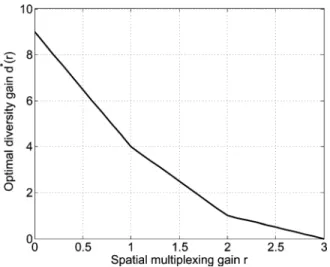
An example of optimal DMT for is given
in Fig. 1. We also remark that there exist space-time lattice codes [5], [17] that are optimal in the DMT sense, i.e., achieve the optimal diversity gain . The condition of in Theorem
Fig. 1. DMT for .
2.1 has been improved to by Elia et al. in [5]. Due to the outstanding error performance of space-time lattices codes, we shall study these codes in general in the next section.
Before concluding this section, we make the following re-mark to further motivate the remainder of this paper. First, while the notion of DMT provides an asymptotic measure of the error performance of the code by focusing on the diversity expo-nent as , there are certain limitations. For example, it is often observed in simulations that two coding schemes and , having the same diversity gain , can differ significantly in error performance when the SNR is fi-nite. In other words, without conducting a simulation it is im-possible to determine which code has better error performance at moderate SNR level from the DMT analysis. This happens es-pecially when the error probability for takes the form
of and similarly
for , and when the functions and behave
like a constant in the asymptotic sense, i.e., in terms of the dotted notations
On the other hand, the above asymptotic ambiguity can be re-solved by the inverse determinant sum, which will be introduced in Section III. Furthermore, it will be seen that the inverse deter-minant sum also represents an alternative, and probably better, criterion for designing STBC in general.
B. Matrix Lattices and Spherically Shaped Coding Schemes
In this paper, we will consider STBC with ,
and therefore these codes live in the space . With this choice, using results from classical lattice theory in , we can define a natural inner product that induces the Frobenius
norm in .
We can “flatten” to obtain a -dimensional
real vector first by forming a vector of length out of the entries (e.g., vectorizing row by row, or column by column) and then by replacing each complex entry with the pair formed by its real and imaginary parts. This defines a mapping from
to :
(7)
which is clearly -linear:
(8)
Let denote the Frobenius norm of .
Note that the following equality holds:
(9) where denotes the Euclidean norm of a vector. This makes an isometry. It also gives us a natural inner product in the
space . Given two matrices , we define
, where the last nota-tion stands for the natural Euclidean inner product in .
Definition 2.2: A matrix lattice has the form
where the matrices are linearly independent over , i.e., form a lattice basis, and is called the rank or the dimension of the lattice.
Definition 2.3: If the minimum determinant of the lattice
is nonzero, i.e., it satisfies
we say that the lattice satisfies the NVD property.
We now consider a spherical shaping scheme based on a -di-mensional lattice inside . Given a positive real number
we define
We will also use the notation
for the sphere with radius .
The following two results are well known.
Lemma 2.2 (Spherical Shaping): Let be a -dimensional lattice in and be defined as above; then
where is some positive constant, independent of .
Proof: For the proof, we refer the reader to [19].
Proposition 2.3: Let be a -dimensional lattice in . Then,
where are constants independent of .
Proof: The proof is a basic exercise in lattice theory. We
In particular, it follows that we can choose real constants and such that
For subsequent discussions, the following definition will be useful.
Definition 2.4: Suppose that is a -dimensional lattice in
. The function , where
is well defined, when and is called the Epstein zeta function [20].
With the above, we are now prepared to give a formal defini-tion of a family of space-time lattice codes of finite size.
Definition 2.5: Given the lattice , a space-time lattice coding scheme associated with is a collection of STBCs where each member is given by
(10) for the desired multiplexing gain and for each level.
The normalization factor in (10) is only appropriate, but not exact, for meeting the average power constraint (3). Specif-ically, one might wonder whether the STBC has average power exceeding the upper constraint in (3). From Proposition 2.3, we have
On the other hand, we also have that from
Proposition 2.2. Combining the above shows that the code has the correct average power from the DMT perspec-tive, i.e., in terms of the dotted equality. Henceforth, we simply ignore the scaling factor of in the channel equation (1) as it is irrelevant to DMT calculations.
III. INVERSEDETERMINANTSUMSOVERMATRIXLATTICES In this section, we introduce inverse determinant sums, study their basic properties and show how they are related to DMT. We first begin with a nonrigorous introduction, which shows how these sums appear naturally as a continuation of more fa-miliar sums.
Consider a -dimensional lattice code for the following additive complex Gaussian noise channel
where and is a length- complex Gaussian random vector with zero mean and covariance matrix .
We have the familiar expression of the pairwise error proba-bility (PEP) upper bound for confusing with at the receiver
If the codewords from the code are sent equiprobably, we can upper bound the average error probability by the following sum:
where the term follows from the fact that we have to con-sider differences of codewords. The right-hand side is indeed a well-known truncated exponential sum taking values on lattice points.
The second example is a quasi-static Rayleigh fading channel with single transmit and receive antennas. Assume that the channel vector is known perfectly to the receiver but not to the transmitter. We then have for the code
and the corresponding upper bound on overall error probability
We can then see that if , the RHS is the truncated Epstein zeta function.
We now turn to the more general case of having a -dimensional NVD lattice and consider a finite code and a slow Rayleigh fading MIMO channel with transmit and receive antennas. The channel equation can then be written as
where and are respectively the channel and noise matrices and where . In terms of PEP, we have for
and the corresponding upper bound on the overall error probability
We summarize the three cases below.
1) Single antenna channel AWGN: is upper bounded by the sum of , an exponential sum.
2) Single antenna slow fading channel: is upper bounded by the sum of , an Epstein zeta function.
3) Quasi-static Rayleigh fading MIMO channel: is upper bounded by the sum of , an inverse determinant sum.
We will see that the behavior of the third sum is the most pecu-liar. While in the second case the limit of the sum for
can be made to converge by increasing , in the last case of inverse determinant sums we will show that they might not con-verge.
A. Basic Problem
Let be a -dimensional lattice. For any fixed , we define
Our main goal is to study the growth of this sum as increases. In particular, we are interested to find, if possible, a function
such that
As we will later see this “dotted” accuracy is enough to deter-mine the DMT of the code under consideration. Furthermore, it gives us a way to select codes with better error performance. Suppose that we have two -dimensional lattices and , and
corresponding functions and
. It is not far fetched to assume that if , the lattice would be a better code, at least for large code sizes. Let us, however, shortly discuss inverse determinant sums in a more accurate sense. Let us denote with the volume of the fundamental parallelotope of a -dimensional lattice in . The normalized version of the inverse determinant sums problem is then to consider the growth of the sum
(11) Here the relevant accuracy level is to find, if possible, functions
and , where , such that
Again it is reasonable to surmise that the smaller the function , the better the corresponding code will be. Comparing codes in this sense does take into account the size of the normal-ized minimum determinant and the number of times this worst-case appears. Obviously, comparing two codes in this normal-ized sense is more reliable than comparing two codes in the pre-viously described dotted sense. However, only in Section IV-D we will consider inverse determinant sums with an accuracy needed for this analysis.
B. Example of the Effect of the Difference in the Growth of Inverse Determinant Sums On the Performance of
Space-Time Codes
The work in this paper is mostly theoretical, but let us give an example that suggests that the inverse determinant sum is also a very practical research subject.
Consider the following lattices:
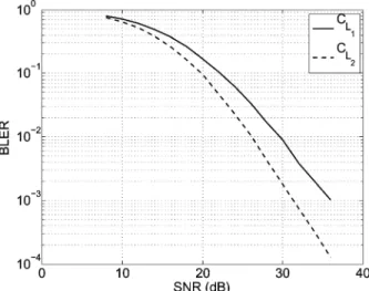
Fig. 2. Block error rates of codes and at 4 bpcu.
Both and are 4-dimensional lattice codes in , and as lattices they are isometric and have exactly the same normal-ized minimum determinant. Suppose that these codes are to be used for communication on a Rayleigh fading channel with a single receive antenna. The corresponding inverse determinant sums are of the type
We will later see that
Here from the normalized minimum determinant and shaping point of view these two codes are identical. Yet, their inverse determinant sums differ dramatically and suggest that the code derived from the lattice has much better error perfor-mance than derived from . The question is whether this difference will be visible in practice. After all, these inverse de-terminant sum considerations have an asymptotic nature.
In Fig. 2, we see the performance of and where the components and takes values in the 16-QAM modulation. It can be clearly seen that performs much better than as predicted by the inverse determinant sums.
C. Elementary Bounds and Some Basic Results for Inverse Determinant Sums
We now provide some simple upper and lower bounds for the asymptotic behavior of for a -dimensional
NVD-lattice in .
Proposition 3.1: Suppose that is a -dimensional NVD-lattice in , with
We then have that
for some constants , , , and .
Proof: Hadamard inequality combined with the arithmetic
mean-geometric mean (AM-GM) inequality gives us
We then have that
Applying Proposition 2.3 yields the lower bounds.
On the other hand, if for all nonzero as
the worst case, then
where is a constant independent of and where the last inequality follows from Lemma 2.2.
We next provide an unsurprising invariance result, revealing that the growth of the inverse determinant sum of a matrix lattice is similar to the corresponding growth of the lattice , where is an invertible matrix in . We need a few lemmas.
Lemma 3.2 [21]: Let and be invertible matrices in
and let be the eigenvalues of and
be the eigenvalues of . We then have that
Lemma 3.3: Suppose that is a set of matrices in and that is an invertible matrix in . If is a function such that for all
then there exists a constant such that for all
where .
Proof: Let be the smallest eigenvalue of . Lemma 3.2 implies that for all the elements ,
. It follows that for the matrix , where
we must have that . We now see that is a
suitable constant for .
Proposition 3.4: Let be a matrix lattice and
be an invertible matrix. If for
some , then
Proof: Let be the smallest eigenvalue of . Using the same argument as in the previous lemma, we have
Changing the roles of and and replacing with give the other direction of the inequality
The previous proposition obviously works also in the case where the lattice is multiplied by a matrix from the right.
D. Inverse Determinant Sum in Relation to DMT
In this section, we will show how we can use DMT to prove lower bounds for the asymptotic growth of inverse determinant sums. At the same time, we will get a criterion for a code to achieve the optimal DMT for multiplexing gains
Let be a -dimensional lattice, and consider the finite codes defined in (10). Assume there are receive antennas. Then, following the union bound together with the PEP-based determinant inequality [22], we get the following bound for the average error probability for the code
(12) The moral of the following proposition is that the determinant sum of a space-time lattice code must grow with considerable speed, or otherwise the code would have DMT exceeding given in Theorem 2.1.
Proposition 3.5: Let be a -dimensional fully diverse lattice in and be a positive integer. Suppose that
for some . We then have that
Proof: Consider the previously mentioned coding scheme
. As we have shown, the union bound (12) yields the following lower bound for :
where . Theorem 2.1, on the other hand, shows that for integer values of
Combining the above gives for integer values of
Hence,
The maximum here is achieved obviously for , but in this case we do not have growth for our matrix sum as the corre-sponding . The next integer point is . In this case, we have
Corollary 3.6: Let be a -dimensional fully diverse lattice. If the corresponding inverse determinant sum achieves the lower bound in Proposition 3.5, then achieves the optimal DMT for , when received with
antennas.
Proof: Here we have
. Setting and
substituting the above into (12) yield
Comparing the above to the DMT lower bound,
for , where is a straight line connecting the points
and yields the desired result.
Remark 3.1: We have stated Proposition 3.5 in the
sim-plest possible form by assuming has a limit
when approaches infinity. While this condition is not that restrictive, the proof of Proposition 3.5 gives us more. It actually states that if there is a function , having
a limit in the dotted sense, for which ,
then . In particular, we
cannot upper bound with any , where
and is some constant.
E. Inverse Determinant Sum and DMT of the Alamouti Code
In this section, we will show that the Alamouti code does reach the bound in Proposition 3.1. This result then allows us to rediscover the DMT of Alamouti code when received with
antennas.
The 2 2 Alamouti code is the following:
for some indeterminate , , , and , where .
The corresponding lattice of the Alamouti code can be written as
which is a 4-dimensional lattice in . We then consider the corresponding inverse determinant sum
Proposition 3.7: Let be a real number. Then,
where and are some constants.
Proof: Due to the orthogonality of the rows of the
Alam-outi code, for any codeword we have
We now have that
The rest follows from Proposition 2.3.
Remark 3.2: In particular, if is large enough the inverse de-terminant sum of the Alamouti code is the Epstein zeta function.
Corollary 3.8: When received with antennas, the Alam-outi code achieves the DMT curve
which is optimal in DMT for any 4-dimensional lattice codec in .
Proof: In order to study the DMT of codes derived from
the lattice , we consider the spherical coding scheme . The usual union bound argument (12) then implies
Also, by Proposition 3.7, we have
where is some constant independent of . This gives us that the Alamouti code does achieve the claimed DMT. The rest fol-lows from [1, Proposition 3.3] where it is shown that this is the best possible for all 4-dimensional lattice codes in .
F. Applying DMT to Lattice Theory
In this section, we give an example showing how Proposition 3.5 can be used in lattice theory.
Let be an 8-dimensional lattice and consider the
Assume that for any nonzero element in . The reader can immediately see that can be reformulated as a matrix lattice and is the absolute value of the determi-nant of 2 2 matrices. We now see what can be said about the asymptotic behavior of the sum
By Proposition 3.1, we have
for some constants and . However, if we can bound the
growth of with any , where and
are constants, then Proposition 3.5 tells us that . This reveals that the lower bound obtained from Proposition 3.5 is considerably stronger than the one from Proposition 3.1 and tells us something nontrivial about the asymptotic behavior of this sum.
However, it should be noted that Proposition 3.5 only applies to the cases when in the sum is an even integer.
We will see that the lower bound is also the best possible in the sense that there are 8-dimensional lattices in for which
It is very likely that there are more direct methods that give this result, but it is intriguing that we can derive such lattice theoretic result from information theory.
IV. INVERSEDETERMINANTSUMS OFALGEBRAICNUMBER FIELDS ANDDMTOFDIAGONALCODES
We now consider inverse determinant sums arising from al-gebraic number field codes [23]. In particular, we will show how the error probability of these codes is tied to the unit group and Dedekind zeta function of the corresponding algebraic number field. These connections allow us to give a better look at the be-havior of these codes and to prove their DMT optimality. The proof of this case will give some insight into the case of codes arising from division algebras.
For simplicity, let us consider a degree cyclic number field extension , where the Galois group is
, and is a principal ideal domain (PID). We will comment more on these conditions in Section IV-D.
We can define a relative canonical embedding of into by
where is an element in . The ring of algebraic integers
has a -basis and therefore
is a -dimensional lattice of matrices in . The main reason to use such a construction is that for each nonzero
el-ement , we have that .
Let be the -dimensional number
field lattice code and consider the coding scheme in (10). Before measuring the DMT for this type of codes, the following definition will be useful. Let be the set of nonzero ideals of the ring . The Dedekind zeta function of the number field
is
(13)
where is a complex number with .
We give the following example for illustration.
Example 4.1: The simplest example of the previous
con-struction arises from the trivial extension . The Ga-lois group then consists simply of the identity element. We then have a lattice , which is a 2-dimensional lattice in . Furthermore, let be the finite code derived from . When received by antennas, the error probability of has a union bound (12) containing the following sum:
The above is actually the truncated Epstein zeta function and the growth of this sum can be analyzed by using Proposition 3.1. However, we can look at this problem from another angle that can be easily generalized. Notice that for every element
, we have , hence
We know that has only four invertible elements
and that is a PID. Therefore, for every ideal , we have exactly four different generators , and . We can then write
which is related to the truncated Dedekind zeta function
at the point . In particular, when we let grow to infinity
we obtain that the sum approaches .
We point out that this approach was earlier taken in [9]. Yet, it only applies to the case when the extension has degree 1. We will next show how this can be extended to more general number fields.
Consider a cyclic extension , where .
With defined as before, let be the finite
code derived from . When received by antennas, the error probability of has a union bound (12) containing the following sum:
where is a set of elements , , each generating a separate ideal in . Accordingly, is the
number of elements , , each generating
the same principal ideal as the one generated by .
If we neglect for the moment the terms , and consider
only the sum , we see that it can be upper
bounded by the truncated Dedekind zeta function at the point .
In the following, we will give bounds for and the truncated sum. The bounds depend only on the value of ; they are independent of the choice of .
A. Bounds for and Truncated Dedekind Zeta Function
We begin our analysis with . This is the number of elements in the unit group of the ring such that
.
Lemma 4.1: Let be a cyclic field extension with . Then, the cardinality of the set
has an upper bound
where is a constant independent of .
Proof: For the ease of reading, the proof to this lemma is
relegated to Section V.
Based on Lemma 4.1, we can upper bound the value of for all .
Proposition 4.2: Let be a cyclic field extension with and let be a nonzero element with . Then,
where is a constant independent of as well as of the ele-ment .
Proof: Given , we can write
. The condition implies
for all . We also have that . It
follows that for all
(15)
Now let be a unit such that
, where
. We have that for all , and (15)
im-plies . Therefore, we have that .
Lemma 4.1 now gives that
where is a constant independent of .
The essential part of this result is that we could find a constant
such that upper-bounds for all
with .
Let us now give a bound for the truncated Dedekind zeta function.
Proposition 4.3: Let be a cyclic field extension with . Then,
(16) where is a subset of in which each element gen-erates a separate integral ideal and satisfies , as defined in (14), and is a constant independent of .
Proof: The proof is relegated to Section V for the ease of
reading.
We remark that if the upper bound in (16) is trivial as the resulting Dedekind zeta function converges to a con-stant, and we can limit the truncated sum that constant. See Section IV-D for a discussion.
B. Inverse Determinant Sum and DMT of Algebraic Number Field Codes
Armed with Propositions 4.2 and 4.3, we are now ready to continue the derivation of (14) to obtain an upper bound for the inverse determinant sum of number field codes.
Proposition 4.4: Let be a cyclic field extension with . Then,
where is some constant independent of .
Proof: Continuing from (14), we have
where the first inequality follows from Proposition 4.2 to upper-bound with a constant , and the second inequality is due to Proposition 4.3 with another constant .
Remark 4.1: Here we have an example of -dimensional lattices where the growth of inverse determinant sums is loga-rithmic. Comparing this bound to that in Proposition 3.1 we can see that we are somewhat close to lower bounds if , but are far from them if . This suggests that the bounds in Proposition 3.1 are not very tight.
Finally, we are ready to determine the DMT curve achieved by number field codes derived from lattice , by which we mean the following. Let be a cyclic field extension of degree
, and consider the -dimensional lattice
be the corresponding finite code obtained by the spherical coding scheme (10).
Theorem 4.5: If the receiver has antennas, the code achieves the following DMT curve:
where .
Proof: Note that is an NVD lattice. It can be easily shown
that the maximal pairwise error probability achieved by
is [1], hence . For the upper
bound on , the usual union bound argument gives
where the last dotted inequality follows from Proposition 4.4 after neglecting the constant factor. Combining the upper and lower bounds on proves the claim.
C. Remark on the Constant Values
In Proposition 4.4, we showed the following result:
For cyclic extensions, where is PID, we point out the as-sumption of being cyclic is not needed anywhere. This bound is also true in the case where is not a PID, but it is only looser. The proof of this result was quite elementary and satisfactory for our purposes, and it can be easily tightened. Below we briefly discuss how our methods can give quite tight asymptotic bounds for number field codes, when the number of receiving antennas is greater than 1.
We note that the term from Proposition 4.3 can simply be replaced with (see the proof of Proposition 4.3), and the function converges to some constant when . This already reduces the bound in Proposition 4.4
to . We can say furthermore a few words
about the constant .
The main theorem in [18] gives us the following asymptotic bound:
(17) where is the number of roots of unity in and is the
regulator.
Let us now prove that uniformly for all nonzero we have
Let be a nonzero element in . We can then write that
where is a diagonal matrix with the property and is a positive constant. This means that , where is extended to a map from (see Section V for a definition) is in the plane generated by some basis of . The lattice has a fixed covering radius . Let us now suppose that is an element in closest to . This means that
. We can now write
This bound is dependent only on and and is therefore
uniform for all .
Assume . By collecting all the previous results, we now have an upper bound
(18) and a lower bound
where . As , (11)
gives us that
and
where . For the PID case,
this bound is probably quite tight asymptotically for the leading term , but generally we are overestimating be-cause by using the Dedekind zeta function we have included in the sum all the ideal classes that might not be principal.
V. SOMEPROOFS OFSECTIONIV
Lemma 4.1 is an elementary corollary to the Dirichlet unit theorem, but we give a proof, as it offers some insight.
Proof of Lemma 4.1: The number field has signature . The Dirichtlet unit theorem then tells us that the unit group has the following multiplicative structure:
where is a finite torsion group containing roots of unity in . Let us consider the mapping
It is well known that is a -dimensional lattice inside .
Consider . If happens to be inside the
for all . It follows that for coordinates having absolute
value greater than 1 we have . On the
other hand, if , we have that
, which is a consequence of the facts that for positive
coordinates and
. In summary, we have for
all .
Therefore, if is inside a ball of radius , then is inside a hypercube with side of length . We have that is a -dimensional lattice, and therefore a
hypercube with side has less than
discrete elements, where is a constant independent of . It
follows that . Now each
of the elements in is a unitary matrix. Hence, for any
with and , we have
. Therefore, we see that
It follows that
As the group is finite, the claim follows.
In the following, we will denote by the set of integral
ideals of the ring .
Proof of Proposition 4.3: Using basic properties of
alge-braic norm and the AM-GM inequality, we have
for any element and . This implies
where is a set of elements , each generating a separate ideal in
From the relation between ideals and element norms, we can further upper bound the above quantity by
where represents the set of all integral ideals. Note that the right-hand-side corresponds exactly to the beginning of the Dedekind zeta function at the point . It then follows that
where the first inequality is based on a similar reasoning as in [24, Proposition 7.2 and Corollary 3] as well as some elementary approximation.
VI. GROWTH OFINVERSEDETERMINANTSUMS OFDIVISION ALGEBRABASEDSPACE-TIMECODES
In this section, we will determine the growth of inverse de-terminant sums of the most well-known algebraic space-time codes. In our main results, we will see that the growth of these sums, and conjecturally also their DMT, only depend on the unit groups of these algebras.
A. Space-Time Codes From Division Algebras
We now recall how to naturally build space-time lattice codes from division algebras. The algebraic results in this section are standard and can be found for example in [25]. Suppose that
or , where is a square free natural
number. Let be a cyclic field extension of degree with
Galois group . Define a cyclic algebra
where is an auxiliary generating element subject to the
relations for all and . We
assume that is a division algebra.
Considering as a right vector space over , every element has the following left regular representation as a matrix :
..
. ...
The mapping is an injective -algebra homomorphism that allows us to identify with its image in . Every nonzero
element in the set is invertible, but is
dense and therefore not directly suitable for space-time coding. An order of a division algebra will offer us a remedy.
Definition 6.1: An -order in is a subring of , having the same identity element as , and such that is a finitely generated module over and generates as a linear space over .
Lemma 6.1: For any element , we have that .
Proposition 6.2: Suppose that . If is a -order in an index- division algebra , then is an -dimensional NVD lattice in , with
for all the elements .
Proposition 6.3: Suppose that . If is an -order in an index- division algebra , then is a -dimensional NVD lattice in , with
Remark 6.1: We note that in both cases an order is also a free -module. This means that we have elements
so that
Therefore,
and we can see that form a basis for the lattice .
The above two families cover many of the most well-known codes. While we will focus only on orders, the corresponding results hold also for principal ideals of orders (see Section IX). For example, the Perfect codes [17] and maximal order codes [26] are of the type described in Proposition 6.3. On the other hand, the Alamouti code and the fast decodable codes in [27] are of the type described in Proposition 6.2.
We now have two families of NVD lattices with and dimensions in , respectively. Below we would like to an-alyze the asymptotic growth of their inverse determinant sums
The analysis will be presented in Sections VI-B and VI-C for the cases of and , respectively. Prior to analyzing the sums, we introduce some central objects needed in both cases.
An obvious lower bound for the growth of an inverse deter-minant sum is given by the number of elements in the set
This set, consisting of elements having the smallest deter-minant in absolute value in the lattice, can be characterized algebraically.
Definition 6.2: The unit group of an order consists of
elements such that there exists with .
Lemma 6.4: If the center of the algebra is or a complex quadratic field, we have that
We can then write
We still need one more object. The following subgroup of will play a crucial part in the analysis of .
Lemma 6.5 ([28, p. 221]): Suppose that the center of the
algebra is or a complex quadratic field. The unit group has a subgroup
and .
The following result reveals why we are interested in the
group .
Lemma 6.6: Let be an index- -central division algebra and be an order in . We then have that
for some constant that is independent of .
Proof: The left side inequality is trivial. The right side is
part of the proof of Proposition 9.3.
In the following sections, we will see that in the dotted sense gives not only a lower bound for the growth of the inverse determinant sum, but also an upper bound!
B. Inverse Determinant Sums of -Central Division Algebras
We first focus on the case where is an index--central division algebra.
The following proposition is an analog to the corresponding result, Proposition 4.4, in the number field case. The proof fol-lows similar lines.
Proposition 6.7: Let be an index- central division algebra
over and be an -order in . Then, for
, we have
where and are constants independent of .
Proof: The proof will be given in Section IX.
We can now see that in order to measure the asymptotic behavior of the determinant sum it is enough to measure the
growth of . However, this is not as simple a
task as in the case of number fields. The unit group is a wild object [28], and we need some advanced tools to solve the problem.
Lemma 6.6 allows us to consider the asymptotic behavior of instead of the whole unit group and translates the problem into solvable form.
Definition 6.3: The set
is the Lie group .
The term cocompact, appearing in the following lemma, will be explained in Section VIII.
Lemma 6.8 [28, Th. 1]: Let be an index- central division
algebra over and an order in . We then
have that
is a discrete cocompact subgroup of .
The reader who is not familiar with these terms can think of an additive lattice inside of . The relation between these ad-ditive groups is similar to that between the multiplicative groups
and .
The previous lemma now identifies the group as a co-compact lattice in , and we can apply the machinery of point counting in Lie groups to prove the following.
Lemma 6.9: Let be an index- central division algebra
Proof: The proof can be found in Appendixes A–D.
We can now combine Proposition 6.7 and Lemma 6.9 for the following.
Theorem 6.10: Let be an index- -central divi-sion algebra and be an order in . Then, for
This result reveals that asymptotically the growth of the in-verse determinant sum of a division algebra-based code only de-pends on the unit group of the underlying order. We can also see that this growth is optimal in the sense that it meets the bound of Proposition 3.5.
The analysis also reveals that all the inverse determinant sums for -central division algebras of index have the same asymptotic behavior.
Remark 6.2: We point out that Proposition 3.5 already told us
that the determinant sums for the algebras of this type must grow at least like . In this section, we showed that this is also an upper bound in the dotted sense. Noting that Proposition 3.5 is based completely on information theory, it is very surprising that the DMT can help to predict the distribution of norms of elements of an order. It appears that the DMT is forcing an order to have a fairly large, that is, dense unit group.
C. Inverse Determinant Sums of -Central Division Algebras
We now concentrate on the case where the center of the di-vision algebra is . The most well-known code of this type is the Alamouti code. Earlier we did analyze the determinant sum of this code by observing that the sum is an Epstein zeta func-tion, and we showed that the growth is in class in the dotted sense. In this section, we will see that this behavior is actually a particular case of a far more general theory.
Suppose that is a -central division algebra and a -order in . Then, is an -dimensional NVD lattice in
.
As in the previous section we have:
Proposition 6.11: Let be an index- -central division algebra and be a -order in . Then, for we have
where and are constants independent of .
Proof: The proof will be given in Section IX-C.
Similar to the previous case, we face the problem of
mea-suring , and again this reduces to measuring
. Promisingly, we can again see as a part
of .
Lemma 6.12: Let be an index- -central division algebra and a -order in . We then have that
is a discrete subgroup of .
Proof: By definition . It is discrete as it is a subset of a discrete set .
The lacking part here is that is not “large enough” to be cocompact in and we cannot directly employ the
methods in Section VIII. Instead we have to make a detour to re-alize the group as part of a “smaller” Lie group that will give us a tight enough fit for the ergodic methods needed for point counting in Lie groups. Unlike the case of complex quadratic centered division algebras, the structure of this algebra will have a dramatic effect on the unit group. Before proceeding, we need some definitions and results.
Consider matrices
where refers to complex conjugation and and are com-plex matrices in . We denote the set of matrices of this type by . Indeed, there is a natural isomorphism between this ring and the ring of matrices over the Hamilton quater-nions .
Definition 6.4: Suppose that is an index- -central divi-sion algebra. If
we say that is not ramified at the infinite place. If and
we say that is ramified at the infinite place.
Lemma 6.13: [25] Suppose that is an index- -central division algebra. Then, has two options. Either it is ramified at the infinite place or it is not.
If the reader is not familiar with tensoring, the main point is that there are exactly two types of central division algebras. Tensoring can then be seen as something that reveals the under-lying geometric structure of the algebra.
Definition 6.5: The set
is a subgroup of the Lie group .
Definition 6.6: The set
is a subgroup of the Lie group .
Lemma 6.14: Suppose we have an index- -central divi-sion algebra and that is a -order in . If is ramified at the infinite place, there exists an invertible matrix
such that
If is not ramified at the infinite place there exists an
invert-ible matrix , such that
Proof: The proof will be given in Section IX-C.
In the following lemma is either or .
Lemma 6.15: Suppose that is an index- -central divi-sion algebra with an order . If is the matrix of
Lemma 6.14, then is a cocompact subgroup in and
Proof: The proof will be given in Section IX-C.
The next lemma now follows as we can apply point counting in Lie groups to the group . Depending of the rami-fication at the infinite place, the counting will be done in
or in .
Lemma 6.16: Let be an index- -central division algebra and be a -order in . If is ramified at the infinite place we have that
If is not ramified at the infinite place, we have
Proof: The proofs will be given in Appendixes A–D.
We can now conclude the following.
Theorem 6.17: Let be an index- -central division al-gebra where the infinite place is not ramified and a -order in
. Then, for we have
Theorem 6.18: Let be an index- , , -central division algebra where the infinite place is ramified. Let be a -order in . Then, for
Remark 6.3: In order to use these results in code design or in
the analysis of known codes, it is crucial to recognize whether the underlying algebra is ramified at the infinite place. We refer the reader to [27] for some simple methods, which will be used in the analysis of the codes in the next example.
Example 6.1: Let us now return to the two example codes
mentioned in Section I: and
. Both of the division algebras have natural or-ders . A straight calculation reveals that these orders have the same geometric structure and normalized min-imum determinant. However, these codes have drastically dif-ferent inverse determinant sums. Corollary 6.18 gives growth
for the code and Corollary 6.17 gives growth
for the code .
VII. COROLLARIES TO THEDMT
It is our belief that the inverse determinant sum of an order code derived from a division algebra indeed describes the DMT of the corresponding coding scheme for multiplexing gain
. In this section, we will turn our inverse-determinant-sum results into lower bounds for the DMT. We will see that in the cases where the DMT of the code is known, the prediction gotten from the inverse determinant sum does give the correct result.
Corollary 7.1: Let be a -central division algebra with index and be a -order in . Then, is an -dimen-sional lattice in . If and is ramified at the infinite place, then the coding scheme derived from lattice based on spherical shaping (10) achieves the DMT curve for
, which is a straight line connecting the points (19) when received by receiving antennas. This curve
coincides with the optimal curve for if and
only if and .
Proof: The DMT lower bound (19) follows directly from
Theorem 6.18 and from an argument similar to the proof of Corollary 3.6. The last statement follows as the optimal DMT curve in the channel, for , is a straight line con-necting the points
Corollary 7.2: Let be a -central division algebra with index and be a -order in . Then, is an -dimen-sional lattice in . If is not ramified at the infinite place, then the coding scheme derived from the lattice based on spherical shaping (10) achieves the DMT curve for
, which is a straight line connecting the points (20) when received by receiving antennas. This curve never coincides with the optimal curve.
Proof: The result follows from Theorem 6.17.
Corollary 7.3: Let be an -central division algebra with
index and . If is an -order inside ,
then is a -dimensional lattice in . The coding scheme derived from lattice based on spherical shaping
(10) achieves the DMT curve for , which is
a straight line connecting the points
when received by receiving antennas. It coincides with
the optimal DMT curve in the range of for any
and .
Proof: The result follows Theorem 6.10.
VIII. POINTCOUNTING INLIEGROUPS
From this section, we begin to work on proving the previously claimed results on determinant sums. As we saw in Section VI, the growth of the inverse determinant sum of a division al-gebra code depends essentially on the asymptotic growth of . The latter can be estimated thanks to the fact that admits a realization as a discrete cocompact sub-group of a suitable Lie sub-group . The term cocompact simply means that the quotient is a compact topological space with respect to the quotient topology.
In this section, we will present some general results on the asymptotic growth of these subgroups.
Let be a Lie group, where is , , or
, and be a discrete cocompact subgroup of . In the following, we will discuss the problem of counting the number of points of that lie inside a sphere defined with respect to the Frobenius norm. We refer the reader to [7] for the relevant definitions and an introduction to the subject. In all the statements in this section, we suppose that is one of the three aforementioned Lie groups. The results of [7] are actually far more general than what is needed in this paper.
Each of the groups admits a Haar measure that gives us a natural concept of volume . In particular, we can consider the volumes of the balls
where here refers to all the matrices in having Frobe-nius norm less than .
The discrete group being cocompact in yields that the measure induced by is finite. A group with this property is called an arithmetic lattice of . This is a natural generalization of an additive lattice in .
The following theorem is stronger than what is needed for measuring the growth of the unit group, but we need this result for the proofs of Propositions 6.7 and 6.11.
Theorem 8.1 ([29], Corollary 1.11 and Remark 1.12):
Con-sider a Lie group , a discrete cocompact subgroup and an element . We then have that
where is some nonzero constant independent of . The limit approaches uniformly for all .
By setting to the identity matrix, one can see that the pre-vious theorem does transform the point counting problem into an integration problem. However, integration on a manifold such as is not completely straightforward.
Theorem 8.2 ([30, Th. 7.4]): Suppose that is a Lie group. We then have that
for some constant .
The value of is well known in the case and
we have that [31]. The corresponding results for and , although probably well known to spe-cialists, are not readily available in the literature, but there are general methods for calculating these asymptotic integrals (see [30] and [32]). In order to use these methods one needs to deter-mine some invariants of Lie algebras, related to the Lie groups under consideration. We explain these technical concepts in
de-tail in Appendix A, where we prove that for
and for , see
Exam-ples A.6, A.7.
IX. PROOFS OFSECTIONVI
In this section, we suppose that the reader is familiar with algebraic number theory and the theory of central simple alge-bras. One should note that we will exclusively work with
max-imal orders. However, the results on the unit groups and growth
of the inverse determinant sums hold also true for other orders. The upper bounds follow as for any order we can find a maximal one such that . On the other hand, the lower bound does come from the density of the unit group and the proofs work for any order and for principal ideals of orders. In particular, our results do cover the Golden code and most of the other perfect codes. This is due to the fact that these codes have the form , where is an order and is a matrix in
. The claim then follows from Lemma 3.4.
A. Some Preliminary Algebraic Results
Let be an index- -central division algebra and a -order in . The (right) Hey zeta function [34] of the order
is
where and is the set of right ideals of . When , this series is converging [35]. However, we can also consider the truncated form of this sum at the point . We have the following lemma.
Lemma 9.1: Let be an index- -central division algebra and be a maximal -order in . If , we have that
for some constants and that are independent of .
Proof: When the sum converges and the bound is trivial. Let us now consider the case when . It first follows from [36, p. 175] where the authors state Hey’s result
where is the Dedekind zeta function defined in (13), and is a function having finite Dirichlet series. In our asymptotic upper bound, we can ignore the term . The terms , for , do stay limited, when approaches 1, and the relevant term is then
where has positive termed Dirichlet series and converges at 1. Generally for truncated positive termed Dirichlet series and and for a positive real number , we have that
where is the formal product of Dirichlet series. This inequality holds even when the series do not converge.
where we consider as a Dirichlet series, with as a variable, and where is a constant independent of . We can now write
where are the coefficients of the original Dirichlet series . Truncating, we have
and in particular
The final result now follows from Proposition 4.3.
B. Proofs of Section VI-B
Let us now concentrate on the case where we have a division algebra with a complex quadratic center . The following lemma will remind the reader of some of the previously men-tioned results and state a crucial relation between the norm and index of elements in . The result is analogous to the corre-sponding one in the number field case.
Lemma 9.2 [25]: If is a maximal -order in an index--central division algebra , then is a -dimensional
lattice in and
(21) where is a nonzero element of .
Lemma 9.3: Let be an index- -central division
al-gebra and an -order in . For any , we have
for some constant , that is independent of and .
Proof: We know that has a finite index inside . Sup-pose that are some representatives of the cosets of the group in . We then have that
As , we can multiply each by a
di-agonal matrix such that and .
Clearly, for all
. According to Theorem 8.1, we then have that
where is independent of and . Now we are ready to prove that
Proof of Proposition 6.7: From the ideal theory of orders
we have that if , then and must differ by a unit. Therefore, we can write
where is a collection of nonzero elements ,
, each generating a separate (right) ideal (and we suppose that does include all elements in ) generating different ideals. According to Lemma 9.3, we can upper bound the previous with
(22) where is some constant independent of .
Using the inequality between Frobenius norm and determi-nant, we have
for any element . Together with (21), this implies that
According to Lemma 9.1, we then have that
where and are some constants independent of . The final result now follows by substituting this into (22).
C. Proofs of Section VI-C
The reader shall notice that in order to keep Section VI-C as simple as possible we postponed the proofs, which can be easily derived from the results in this section.
Suppose that is an index- -central division algebra and a -order. We are now interested in the behavior of the determinant sum
However, unlike in the case where the center is complex quadratic, we cannot approach the problem directly. Instead we will use another, geometrically more revealing, embedding (to be defined later) and we will study the corresponding sum
In the end, we will prove that the behavior of this sum com-pletely describes the behavior of the original sum, too.
Recall that there are exactly two options for a -central divi-sion algebra , either
or
In both cases, we will denote the corresponding isomorphisms by . With abuse of notation, we define
for .
Lemma 9.4 [25]: If is a maximal -order in an index--central division algebra , then is an -dimensional
NVD lattice in and
(23) Now, we can proceed just as in the case of division algebra with complex quadratic center.
Proposition 9.5: Let be an index- -central division al-gebra and be a maximal -order in . Then, for
we have
where and are constants independent of .
In the following, we will denote and by .
Just as in the case of , we have the following.
Lemma 9.6 [28, Th. 1]: Suppose that is a -central divi-sion algebra and a -order in . We then have that
is a cocompact lattice in .
Using point counting in Lie groups, we now have:
Proposition 9.7: Let be an index- -central division al-gebra and a maximal -order in . Then, for
According to Examples A.6 and A.7, we now have the fol-lowing desired results.
Corollary 9.8: Let be an index- -central division al-gebra where the infinite place is not ramified and a maximal
-order in . Then, for we have
Corollary 9.9: Let be an index- , , -central division algebra where the infinite place is ramified. Let be a maximal
-order in . Then, for
We are now ready to return to the original embedding of the division algebra.
Lemma 9.10: Suppose that is an index- -central divi-sion algebra and that is a -order in . Then, there exists
such that
for every element .
Proof: We can build a well-defined mapping
where and is the identity
ma-trix. It is then easy to prove that this is a bijective -algebra homomorphism.
We also have a -algebra morphism ,
where . This is just as well a bijection.
The Skolem Noether theorem now states that there exists an
invertible matrix , such that
for every element in . In particular, we have that .
Proposition 9.11: Suppose that is a -central division al-gebra and that is a -order in we then have that
Proof: Combining Lemma 9.10 and Proposition 3.4 gives
us this result.
Theorems 6.18 and 6.17 now directly follow from Corollaries 9.8 and 9.9.
X. CONCLUDINGREMARKS AND SUGGESTIONS FORFURTHERWORK
In this paper, we laid a basis for studying inverse determi-nant sums and developed methods for analyzing inverse deter-minant sums and DMTs of large families of algebraic codes. We introduced several techniques, not used before in algebraic space-time coding, and revealed surprisingly tight connections between information theoretic and algebraic concepts.
There are now several directions where this study can be continued. Let us shortly describe a few of them. The most straightforward problem is the tightening of the results we have gotten, so that we can make a difference between codes that in the rough asymptotic sense, which we have mostly focused on, are similar. Preliminary research suggests that our methods can be sharpened to consider also the sums , introduced in Section III-A. Can these more refined methods then be used to find the division algebras that yield the optimal growth for the
corresponding sums ?
It seems to be that the growth of an inverse determinant sum always describes the DMT of a minimum delay space-time code for multiplexing gains . Can this be proved or dis-proved? Can one give a more direct proof for the results in Section III-F?
APPENDIX
COMPLEX ANDREALLIEALGEBRAS, ROOTSYSTEMS AND HIGHESTWEIGHT
The aim of this appendix is to compute the constant in
The-orem 8.2 when the group is , , or .
In order to do so, we need some basic facts about Lie algebras. For a general introduction to Lie algebras and beyond, we refer the reader to [38], [39].
A (finite dimensional) Lie algebra over the field is a fi-nite-dimensional vector space over endowed with a bilinear product , called the Lie bracket, such that
and satisfying the Jacobi identity
For any Lie algebra , we can define a mapping
such that , , and a bilinear form
(Killing form) on given by . We
will only consider the case where is equal to or . In this case, is semisimple if the Killing form is nondegenerate. We will say that is Abelian if , or equivalently,
Even though we are mainly interested in real Lie algebras, it will be easier to define the notions of root system and weights in the case of complex Lie algebras and then derive the corresponding definitions for the real case.
Notation: We denote by the standard basis of and by the corresponding dual basis. To simplify
notation, we write and . We will always
suppose that in the sequel.
A) Root Space Decomposition and Irreducible Represen-tations of Complex Lie Algebras: Let be a semisimple Lie algebra over . A Cartan subalgebra is a maximal Abelian subalgebra such that , is diagonalizable. Given a Cartan subalgebra , let be its dual as a vector space.
For , let
If , we say that is a root of (or simply a root of with abuse of notation). We denote the set of all roots of by . The following root space decomposition holds:
(24) Consider the -vector space
(25)
One can show that , so that an basis of
over is also a basis of over . Every choice of an ordered basis of induces a partition of the roots into positive and negative roots as follows.
Given a root , we write if such that
for and , and
otherwise [39]. We denote the set of positive roots by . A positive root is called simple if it cannot be written as a sum of positive roots. We denote the set of simple roots by . Now consider a complex representation of , that is a
mor-phism where is a finite-dimensional complex
vector space. Here viewed as a Lie algebra
with the commutator as Lie bracket.
A subspace is invariant under the representation
if , . The representation is irreducible
if does not contain any nontrivial invariant subspace.
Given , we define
If we say that is a weight. Let be the set of
weights: then we have the weight space decomposition
A highest weight vector is a nonzero vector that belongs to
some weight space and such that ,
. In this case, is called a highest weight. It can be shown that every finite-dimensional representation of a semisimple Lie algebra admits a highest weight vector; the highest weight vectors of an irreducible representation of are unique up to multiplication by nonzero scalars. Equivalently, the highest weight is unique and the corresponding weight space is 1-dimensional.
Example A.1 ( as a Complex Lie Algebra):
The complex Lie algebra corresponding to the Lie group is
with the Lie bracket . One can show that
it is semisimple; the set of trace zero diagonal matrices is a Cartan subalgebra; it is a vector space of dimension over
. We choose the ordered basis of
.
Note that for , if we consider two elements
, , we
have ,
(26) so is diagonal with diagonal elements , and
It is not hard to see that the set of roots is
In fact, from (26) we find that , is contained in the root space with . By (24), all the root spaces are 1-dimensional and of the form . Moreover,