過度反應或反應不足？台股之濾嘴法則實證研究 - 政大學術集成

全文

(1)國立政治大學國際經營與貿易學系碩士論文. 過度反應或反應不足？台股之濾嘴法則實證研究. 治政大 Overreaction or Underreaction? : 立 ‧ 國. 學. Empirical Study on the Application of Filter Rule to Taiwan Stock Market. ‧. io. sit. y. Nat. n. er. 指導教授：郭炳伸 i博士 al v Ch. n U engchi. 研究生：嚴浩祖. 撰. 中華民國一百零二年六月.

(2) 謝辭此份學業的完成受到許多人幫助。謝謝我的父母對我無保留支持，並給予我自由發展的空間。謝謝郭炳伸老師在論文上的指導，且耐心幫助我修改英文文句。謝謝王植婷小姐協助我逐一審視英文文法。謝謝郭維裕老師與蔡文禎老師在口試時的建議，還有這一路上與一些朋友共同的學習成長。最後也感謝自己，願意嘗試用英文寫作，即使過程辛苦，. 治政也證實了自己願意面對挑戰；而交換學生的過程更讓我有了寶貴的經驗，大立 ‧. ‧ 國. 學. 生命教導了我許多事。. n. er. io. sit. y. Nat. al. Ch. engchi. i n U. v.

(3) 摘要本論文以濾嘴法則應用在台灣股票市場，試圖揭露報酬率與成交量之間的關係。雖然在短期內可藉由過度反應獲取報酬，然而，報酬率與成交量的關係仍舊模糊不清，本篇引用的文獻並不足以解釋此研究的結果。另外，我們發現在近十年中，因流動性進行的交易，而非因資訊進行的交易，主導了台灣股票市場。. 立. 政治大. ‧. ‧ 國. 學. 關鍵詞：成交量、價量關係、過度反應. n. er. io. sit. y. Nat. al. Ch. engchi. i n U. v.

(4) Abstract This thesis uses filter rule on Taiwan stock market to uncover the relationship between return and volume change. Although the profits for overreaction in a short time horizon exist, the pattern of the combination of return and volume change is unclear. No theory mentioned in the literature seems to be able to fully explain the results in this study. Yet, we find that the liquidity trading, rather than information trading, dominates Taiwan stock market in recent decade.. 立. 政治大. Keywords: volume, return, overreaction. ‧. ‧ 國. 學. n. er. io. sit. y. Nat. al. Ch. engchi. i n U. v.

(5) 1. Contents CHAPTER I.. INTRODUCTION .............................................................................. 5. CHAPTER II.. REVIEW OF RELATED THEORY .........................................................10. CHAPTER III. EMPIRICAL STRATEGY AND METHODOLOGY ...................................13 CHAPTER IV. EMPIRICAL FINDINGS .....................................................................17 IV.I. DATA ............................................................................................................... 17. IV.2. ONE-WEEK FILTER ............................................................................................. 17. IV.3. TWO-WEEK FILTER ............................................................................................. 20. IV.4. TWO-DAY FILTER ............................................................................................... 24. IV.5. TWO PERIODS OF TIME ....................................................................................... 28. IV.6. DISCUSSION ..................................................................................................... 29. 立. ‧. ‧ 國. 學. CONCLUSIONS ...............................................................................32. io. sit. y. Nat. n. al. er. CHAPTER V.. 政治大. Ch. engchi. i n U. v.

(6) 2. Table Contents TABLE I RESULTS FOR THE CASE WHERE PROFITS ARE CALCULATED ONE WEEK AFTER THE STRATEGY-FORMED-DAY, AND LAGGED RETURN AND VOLUME CHANGE ARE CALCULATED IN THE PREVIOUS WEEK, 1993-2012 ..................................................................................... 34 TABLE II RESULTS FOR THE CASE WHERE PROFITS ARE CALCULATED TWO WEEKS AFTER THE STRATEGY-FORMED-DAY, AND LAGGED RETURN AND VOLUME CHANGE ARE CALCULATED IN THE PREVIOUS WEEK, 1993-2012 ..................................................................................... 35 TABLE III RESULTS FOR THE CASE WHERE PROFITS ARE CALCULATED THREE WEEKS AFTER THE STRATEGY-FORMED-DAY, AND LAGGED RETURN AND VOLUME CHANGE ARE CALCULATED IN THE PREVIOUS WEEK, 1993-2012 ..................................................................................... 36. 立. 政治大. TABLE IV RESULTS FOR THE CASE WHERE PROFITS ARE CALCULATED FOUR WEEKS AFTER THE STRATEGY-FORMED-DAY, AND LAGGED RETURN AND VOLUME CHANGE ARE CALCULATED IN THE. ‧ 國. 學. PREVIOUS WEEK, 1993-2012 ..................................................................................... 37. TABLE V RESULTS FOR THE CASE WHERE PROFITS ARE CALCULATED ONE WEEK AFTER THE. ‧. STRATEGY-FORMED-DAY, AND LAGGED RETURN AND VOLUME CHANGE ARE CALCULATED IN THE PREVIOUS TWO WEEKS, 1993-2012 ............................................................................ 38. y. Nat. sit. al. er. io. TABLE VI RESULTS FOR THE CASE WHERE PROFITS ARE CALCULATED TWO WEEKS AFTER THE STRATEGY-FORMED-DAY, AND LAGGED RETURN AND VOLUME CHANGE ARE CALCULATED IN THE PREVIOUS TWO WEEKS, 1993-2012 ............................................................................ 39. n. v i n C hPROFITS ARE CALCULATED TABLE VII RESULTS FOR THE CASE WHERE e n g c h i U THREE WEEKS AFTER THE STRATEGY-FORMED-DAY, AND LAGGED RETURN AND VOLUME CHANGE ARE CALCULATED IN THE. PREVIOUS TWO WEEKS, 1993-2012 ............................................................................ 40. TABLE VIII RESULTS FOR THE CASE WHERE PROFITS ARE CALCULATED FOUR WEEKS AFTER THE STRATEGY-FORMED-DAY, AND LAGGED RETURN AND VOLUME CHANGE ARE CALCULATED IN THE PREVIOUS TWO WEEKS, 1993-2012 ............................................................................ 41 TABLE IX RESULTS FOR THE CASE WHERE PROFITS ARE CALCULATED TWO DAYS AFTER THE STRATEGY-FORMED-DAY, AND LAGGED RETURN AND VOLUME CHANGE ARE CALCULATED IN THE PREVIOUS TWO DAYS, 1993-2012 ............................................................................... 42 TABLE X RESULTS FOR THE CASE WHERE PROFITS ARE CALCULATED FOUR DAYS AFTER THE STRATEGY-FORMED-DAY, AND LAGGED RETURN AND VOLUME CHANGE ARE CALCULATED IN THE PREVIOUS TWO DAYS, 1993-2012 ............................................................................... 43.

(7) 3. TABLE XI RESULTS FOR THE CASE WHERE PROFITS ARE CALCULATED SIX DAYS AFTER THE STRATEGY-FORMED-DAY, AND LAGGED RETURN AND VOLUME CHANGE ARE CALCULATED IN THE PREVIOUS TWO DAYS, 1993-2012 ............................................................................... 44 TABLE XII RESULTS FOR THE CASE WHERE PROFITS ARE CALCULATED TWO WEEKS AFTER THE STRATEGY-FORMED-DAY, AND LAGGED RETURN AND VOLUME CHANGE ARE CALCULATED IN THE PREVIOUS TWO WEEKS, 1993-2002 ............................................................................ 45 TABLE XIII RESULTS FOR THE CASE WHERE PROFITS ARE CALCULATED TWO WEEKS AFTER THE STRATEGY-FORMED-DAY, AND LAGGED RETURN AND VOLUME CHANGE ARE CALCULATED IN THE PREVIOUS TWO WEEKS, 2003-2012 ............................................................................ 46 TABLE XIV RESULTS FOR THE CASE WHERE PROFITS ARE CALCULATED TWO DAYS AFTER THE STRATEGY-FORMED-DAY, AND LAGGED RETURN AND VOLUME CHANGE ARE CALCULATED IN THE PREVIOUS TWO DAYS, 1993-2002 ............................................................................... 47. 立. 政治大. ‧. ‧ 國. 學. TABLE XV RESULTS FOR THE CASE WHERE PROFITS ARE CALCULATED TWO DAYS AFTER THE STRATEGY-FORMED-DAY, AND LAGGED RETURN AND VOLUME CHANGE ARE CALCULATED IN THE PREVIOUS TWO DAYS, 2003-2012 ............................................................................... 48. n. er. io. sit. y. Nat. al. Ch. engchi. i n U. v.

(8) 4. Figure Contents. FIGURE I. EXPECTATION FROM WANG’S THEORY ..................................................................... 11 FIGURE II. EMPIRICAL STRATEGY AND METHODOLOGY ............................................................. 13 FIGURE III. RETURN OF TWO-WEEK FILTER STRATEGY ............................................................... 23 FIGURE IV. RETURN OF TWO-DAY FILTER STRATEGY .................................................................. 27 FIGURE V. THE SHAREHOLDING RATIO OF QUALIFIED FOREIGN INSTITUTION INVESTORS .................. 30. 立. 政治大. ‧. ‧ 國. 學. n. er. io. sit. y. Nat. al. Ch. engchi. i n U. v.

(9) 5. Chapter I.. Introduction. The technical analysis has been used in trading for many decades. Many evidence shows it is profitable. Traders may make profits with momentum or contrarian strategy. The information used in the original and. 政治大. basic technical analysis is based on price. Lehmann (1990) points out that. 立. using contrarian strategy based on the return of previous week can earn. ‧ 國. 學. profits on the following week. His explanation is that fundamental valuation does not change over a short time interval such as a week. Even though. ‧. many scholars attribute Lehmann’s result to bid-ask bounce or other reasons,. y. sit. Nat. Cooper (1999) uses filter rule to filter out the noise, whose lagged return. er. io. does not move down or up by a minimum amount, and document large and. n. a consistent profits. Moreover, Cooper incorporates lagged trading volume v. i l C n U in theory that traders into filter. Blume, Easley, and h O’Hara e n g(1994) c h i suggest who include trading volume into their analysis perform better than those who do not. There is an adage in the practical realm that says: price follows volume. Not only in Taiwan stock market, but also similar saying in U.S. stock market. Traders see trading volume as an indicator for the price momentum. Cooper (1999) uses filter rule technical analysis and tries to illustrate the relationship between price and volume. He mainly cites two papers with.

(10) 6. opposite implications for the role of trading volume, Campbell, Grossman, and Wang (1993) and Wang (1994). Campbell, Grossman, and Wang (1993) develop a model in which the risk-averse utility maximizers play a role like market maker, and the market information is symmetric. When some investors sell their stocks out of exogenous pressure, like liquidity, other risk-averse utility-maximized investors are willing to accommodate the selling pressure, but will require a higher expected return. The deviation from the original price, because of. 政治大 the stocks. Thus, their model predicts that price changes with high volume 立. liquidity trading, is not due to the change of the fundamental valuation of. will tend to be reversed in the future.. ‧ 國. 學. On the other hand, Wang (1994) indicates another scenario. There. ‧. might be a different relationship between price and volume if the market is. sit. y. Nat. with information asymmetry. In this case, there are two types of investors:. io. er. informed and uninformed investors. Informed investors can trade for informational or noninformational purpose. Wang hypothesized when. al. n. v i n trade onCtheir information, price change, with U h e nprivate i h gc. informed investors. high trading volume, tends to continue in the same way in the future.. Simply put, Campbell, Grossman, and Wang (1993) hypothesize that in an information symmetric market where investors trade for liquidity purpose, return tends to be reversed when there is high trading volume. Instead, Wang (1994) hypothesizes that in an information asymmetric market where investors are trading on their internal information, return tends to continue until all the information is disclosed when there is high trading volume. Based on these predictions, Cooper (1999) uses the stocks for the top.

(11) 7. 300 largest market capitalization in the U.S. stock market between 1962 and 1993. He collected information on the return and volume change in the previous week for his filter rule. He found that “decreasing-volume stocks experience greater reversals” and “increasing-volume stocks exhibit weaker reversals and positive autocorrelation” [Cooper (1999, p.901)]. The reversals from decreasing-volume were explained by Cooper as “period of portfolio rebalancing for both informed and uninformed investors” [Cooper (1999, p.920)], while the weaker reversals and positive autocorrelation from. 政治大 This thesis mainly uses the same methodology of Cooper’s. The size 立. increasing-volume corresponds to the hypothesis of Wang (1994) proposed.. and in history the development of Taiwan stock market are not as large and. ‧ 國. 學. long as of U.S. stock market. A small market could be influenced easily by. ‧. some traders when they trade for internal information. If a market is not. sit. y. Nat. fully developed, and if a market is not well regulated, internal information. io. er. would be often exploited to trade. Accordingly, I presume that Taiwan stock market is much more information asymmetric than U.S stock market, and. al. n. v i n expect that the same patternCas Cooper (1999)’s in Taiwan’s stock market he ngchi U might be established as well.. However, there is a related article indicating another different role for trading volume. Gervais, Kaniel, Mingelgrin (2001) assume that volume reflects a given stock’s visibility and can be the price premium. Their assumption is based on the claim of Miller (1977) and Mayshar (1983) that the holders of a stock tend to be more optimistic about the stock’s prospect. Gervais, Kaniel, Mingelgrin find that even with little or no price change, volume can be used to predict future price change, i.e. volume itself can be an exclusive predictor, does not need to be accompanied with return. A stock.

(12) 8. experiencing unusually high (low) trading volume tends to appreciate (depreciate) in the future. This finding is not however fully consistent with Cooper’s finding. This is because the stocks experiencing unusually high trading volume and low return tend to exhibit weaker reversals and even positive autocorrelation, not appreciate, in his finding; and those experiencing low trading volume and low return tend to be reversed, not depreciate. Nevertheless, the window set in of Cooper’s finding is one week; and that in Gervais, Kaniel,. 政治大 result might vary if Cooper prolongs the window. This motivates this study 立. Mingelgrin’s finding is more than one week, or even many months. The. to extend the window and to see whether Cooper’s finding holds for the next. ‧ 國. 學. few weeks.. ‧. Like Lehmann (1990), Kelley (2004) also discusses the contrarian. y. Nat. strategy. Although he only uses price change as a filter to form his portfolio,. er. io. sit. buying previous week’s loser and selling previous week’s winner, he still found evidence for the contrarian: return of winner tends to be negative,. al. n. v i n C hbe positive. In addition, while return of loser tends to he suggests that, for engchi U. the first four weeks, extreme winner is predicted to turn to negative return, and extreme loser to positive return. After four weeks of time, the contrary would disappear, and original extreme return would continue; namely. winner still wins whereas loser still loses, which lasts for almost a year. When stock price is reversed, it means overreaction of the original return; but when the stock price stops reversal and continues its original price trend, that implies underreaction. It remains unclear if the overreaction Cooper found will turn out to be underreaction when the window is prolonged, another justification that the window is extended in the study..

(13) 9. There are also a few studies using filter rule on return and volume change of Taiwan stock market to examine the future return. One is Hsu (2004), using slightly-changed filter rule to examine Taiwan Stock Exchange Capitalization Weighted Stock Index future contracts. His empirical evidence shows that price trend is predictable when “the noise” is filtered out, and the combination filters of price and volume display more predictability than those only with price change. Chen (2006) use filter rule on Taiwan Stock Exchange Capitalization Weighted Stock Index. He. 政治大 A few important findings emerge from this study. First, in a relatively 立. obtained similar result to that found in Cooper’s, though not so significant.. short time horizon, lagged return is a better return predictor than lagged. ‧ 國. 學. volume. But, in a longer time horizon, return tends to be negative if the. ‧. lagged volume extremely decreases. Second, return and volume change in. sit. y. Nat. two weeks of time are more powerful to predict the future return than that in. io. er. one week. Third, when we use return and volume change in two days of time to predict future returns, we find that decreasing-volume stocks. al. n. v i n C hand increasing-volume reversals engchi U. experience greater. stocks experience. reduced reversals. Fourth, when we use return and volume change in two weeks of time to predict future returns, we find that a simultaneous increase in return and volume change would be followed by an increase in return. Fifth, Taiwan stock market is likely to be more dominated by liquidity trading than information trading in recent decade. The remainder of this thesis is organized as follows. Chapter II describes the related theories and presents the hypothesis to be tested. Chapter III explains empirical strategy and methodology to be used. Chapter IV gives empirical findings. Chapter V concludes..

(14) 10. Chapter II. Review of Related Theory. This chapter explains how trading volume plays a different role in theory between Campbell, Grossman, Wang (1993) and Wang (1994). We would like. 政治大. to find the empirical evidence to test these theories.. 立. In an information asymmetric market as Wang (1994) hypothesized,. ‧ 國. 學. informed and uninformed investors exist at the same time. They are all heterogeneous in their information about the stock’s future dividends, private. ‧. investment opportunities, and so forth. When the information arrives, the. y. sit. Nat. difference in investors’ response to the same information generates tradings.. er. io. The informed investors update their expectations differently. The. n. uninformed investors areawilling to trade with informed i v investors since some. l C n U h trades from informed investors are e nalso h i motivated. g cliquidity. Therefore, the. greater the information asymmetry, the larger the abnormal trading volume when information arrives. When the news about the future dividend is disclosed after uninformed investors’ trading with informed investors, uninformed investors realize the mistakes in their previous trading with informed investors that they have underestimated the value of the stock as the true state is revealed. They would trade to revise the positions, and that would push the stock price to go further. Thus “a high return accompanied by high volume implies high future returns”.

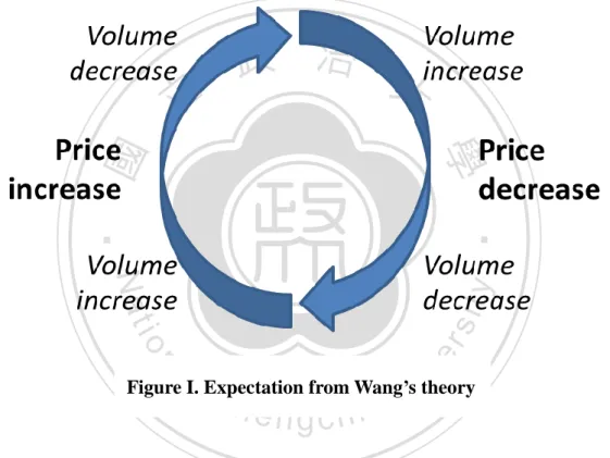
(15) 11. [Wang (1994, p.130)] if the informational trading dominates. Figure I summarizes the mechanism in Wang’s model. In an information asymmetric market, when the return is accompanied by high volume, return tends to continue. When the return is accompanied by low volume, as explained by Cooper as “period of portfolio rebalancing for both informed and uninformed investors” [Cooper (1999, p.920)], return tends to be reversed.. 立. 政治大. ‧. ‧ 國. 學. n. er. io. sit. y. Nat. al. Ch. i n U. v. Figure I. Expectation from Wang’s theory. engchi. If the market is information symmetric, which Campbell, Grossman, Wang (1993) assume, the liquidity trading dominates. Some investors trade for liquidity or noninformational purpose, and they sell their stocks for exogenous pressure. Other investors act like market makers in the sense that “they are willing to accommodate the selling pressure, but that they demand a reward in the form of a lower stock price and a higher expected stock return” [Campbell, Grossman, Wang (1993, p.905)]. When investors sell their.

(16) 12. positions due to exogenous pressure, because the value of the stocks does not change in a short time period, the price tends to be reversed. Their model suggests that price changes accompanied by high volume tend to be reversed. The major difference between Campbell, Grossman, Wang (1993) and Wang (1994) is to assume whether market is information symmetric or asymmetric. The return accompanied by high volume tends to be reversed in Campbell, Grossman, Wang (1993) and tends to continue in Wang (1994). The size of Taiwan stock market is much smaller than that of U.S. stock. 政治大. market. Information asymmetry would be more severe in this situation.. 立. Therefore, information shared between informed traders and non-informed. ‧ 國. 學. ones is expected to be more asymmetric in Taiwan than in the U.S. It is reasonable that the evidence uncovered using data from Taiwan stock market. ‧. may as well be in support of Wang’s theory, as that of Cooper’s. This is the. y. Nat. n. al. er. io. sit. topic of the study that we will pursue in the next chapters.. Ch. engchi. i n U. v.

(17) 13. Chapter III. Empirical Strategy and Methodology. 政治大 starts with collecting information in a weekly basis. Each trading strategy is 立 The study employs the same filter rule as in Cooper (1999). My analysis. ‧ 國. 學. formed based on the return and volume growth up to week t – 1, one week. before the strategy is formed, and the return resulting from the implementation. ‧. of the strategy is calculated in the following weeks.. n. er. io. sit. y. Nat. al. Ch. engchi. i n U. v. Figure II. Empirical strategy and methodology. If a stock’s return is positive in week t - 1, it is called “winner”, and “loser” if negative. The lagged return grid width, for either “winner” or.

(18) 14. “loser”, equals 2%. These filter rules are defined as follows: Price Filters: Return states = loser if - k*A > Ri,t-1 >= -( k+1)*A, for k = 0, 1, …, 4 winner if k*A <= Ri,t-1 < (k+1)*A, for k = 0, 1, …, 4 loser if Ri,t-1 < - k*A, for k = 5 winner if Ri,t-1 >= k*A, for k = 5 where Ri,t-1 is return for security in week t - 1, k is the filter counter that ranges from 0 to 5 and A is the lagged return grid width, equal to 2%. I use. 政治大. close price on Tuesday to calculate the return.. 立. For example, if the return is -5%, it would belong to the filter which is. ‧ 國. 學. larger than or equal to -6%, and smaller than -4%. If the return is 13%, it would belong to the filter which is larger than or equal to 10%.. ‧. I also use growth in volume as filter:. y. Nat. io. sit. %ΔVi,t = ( Vi,t - Vi,t-1 ) / Vi,t-1,. a. er. where Vi,t is the average daily volume for security i in week t. Average daily. n. i v possibility of holidays l volume, to excludenthe volume, instead of total weekly. Ch. U i e h n c g falling on weekdays is used. If a stock’s growth in volume, %ΔVi,t-1, in week t - 1 is positive, it is defined as “high-volume”, and negative, “low-volume”. These rules are defined in detail as follows: Volume filters: Growth in volume states= low if – k*B > Ri,t-1 >= -( k+1)*B, for k = 0, 1, 2, 3 high if k*C <= Ri,t-1 < (k+1)*C, for k = 0, 1, 2, 3 low if Ri,t-1 < -k*B, for k = 4 high if Ri,t-1 >= k*C, for k = 4.

(19) 15. where k refers to the filter counter that ranges from 0 to 3, B is the grid width for low growth in volume and is equal to 15%, and C is the grid width for high growth in volume and is equal to 30%. The asymmetry of the choice of the grid width for high- and low-volume is due to skewness in growth in volume distribution. For example, if the volume change is -62%, it would belong to the filter which is smaller than -60%. If the volume change is 100%, it would belong to the filter which is larger than or equal to 90%, and smaller than 120%.. 政治大. The example that follows is to give a concrete idea of how the filter rule. 立. works. For example, suppose 12/18 is Tuesday, so I use the close prices on. ‧ 國. 學. 12/11 and 12/18 respectively to calculate the return for that week, denoting. 12/12 to 12/18 to see the growth in volume, %ΔVi,t-1.. Nat. y. ‧. Ri,t-1. I also calculate the average daily volume from 12/5 to 12/11 and from. io. sit. The securities whose lagged return and volume change meet the same. a. er. filter are formed into the same portfolio with equal weight. Namely, the. n. v returns which fall into the lsame filter will be summed n i up and divided by the Ch. U i e h n c g number of stocks when calculating the average mean, regardless of the size or the price of stocks.. Then, I use the open price on Wednesday as the holding cost. In the case of holding for one week, I use the open price on the next Wednesday, 12/26, as exit price to see if there is any pattern that can be observed in the return, based on the filter Ri,t-1 and %ΔVi,t-1. In the case that Tuesday is a holiday, I take the close price on Monday to calculate return. A close price on Tuesday for next or previous week is still.

(20) 16. used. If Wednesday is a holiday, I take the open price on Thursday as holding cost or exit price. An open price on Wednesday for next or previous week is still set to be holding cost or exit price. The measure of volume will be less influenced by holidays, because of its averaging nature.. 立. 政治大. ‧. ‧ 國. 學. n. er. io. sit. y. Nat. al. Ch. engchi. i n U. v.

(21) 17. Chapter IV. Empirical Findings. This chapter presents the major empirical findings for the proposed filters, and reports as well as discusses the results at the end of this chapter.. 政治大. 立 IV.I. Data. ‧ 國. 學. I select top 50 largest capitalization stocks of listed companies every year. ‧. from 1993/1/5 to 2012/12/28, a total of 5225 trading days in Taiwan Stock. sit. y. Nat. Exchange Market. If one stock suspends trading, the data that are 10 days. er. io. before and after the suspension will not be included. The list of top 50 largest. n. a companies is updated oni v the first trading day of capitalization stocks of listed. l C n U h every year. By using top 50 largest e capitalization n g c h i stocks, the return caused by bid-ask bounce can be avoided.. IV.2. One-week filter Return filter. At the beginning, we begin with examining the results for filters with only lagged return. Table I presents results for the case where profits are.

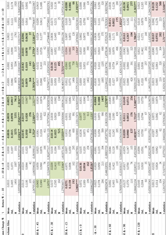
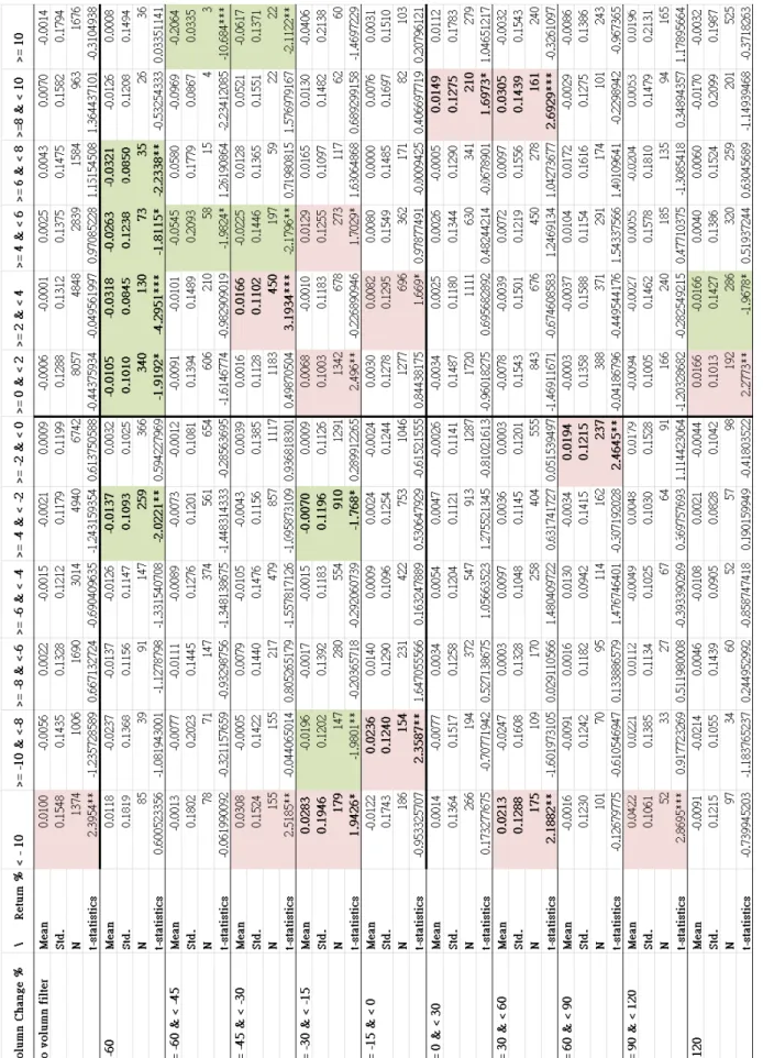
(22) 18. calculated one week after the strategy-formed-day. As clearly seen from the Table, just a few instances of returns are statistically significant. Cooper also uses lagged return filter, and his results show reversals in the loser and winner portfolios. In his paper, although not all the returns of winner filters are statistically significant, those of loser filters are. That is very different from our results. Table II presents the results for the case where profits are calculated two weeks after the strategy-formed-day. It shows that with not too much price. 政治大. decrease in the previous week, the returns turn negative and significant.. 立. Same results can be seen in Table III, presenting the results for the case. ‧ 國. 學. where profits are calculated three weeks after the strategy-formed-day. Also, Table III shows that with moderate increase in price in the previous week, the. ‧. returns turn positive and significant three weeks after the strategy-formed-day.. y. Nat. a. er. io. strategy-formed-day.. sit. It is puzzling why this takes place just three weeks after the. n. v Results for the casesl where profits are calculated n i four weeks after the Ch. U i e h n c g strategy-formed-day are collected in Table IV. Almost all of the past instances of significant returns are not significant anymore.. The results may show some evidence for predictability, but it is also not consistently that some instances of results are only significant at sometimes and do not consistent with the previous or following week.. Return and volume filter Under the lagged return filter space in the table, there are four quadrants.

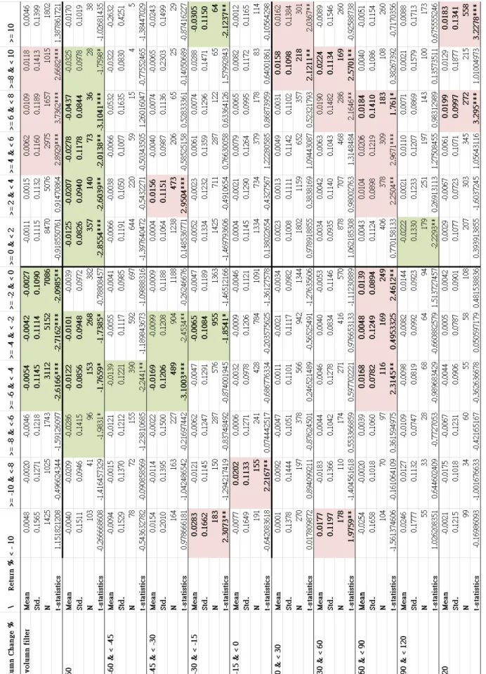
(23) 19. of filters combined with the lagged return and the lagged volume change. The first quadrant is “winner, low-volume” strategy on the upper right; the second is “loser, low-volume” on the upper left; the third is “loser, high-volume” on the lower left; the fourth is “winner, high-volume” on the lower right. My expectation is when there is high trading volume, the return tends to continue; and when there is low trading volume, the return tends to be reversed. Nevertheless, the results on these four quadrants from Table I to IV are not so significant. Throughout these four tables, the maximum number of. 政治大. significant filters is 30 out of 120, which is very dissimilar to Cooper’s results.. 立. In Table I, there is not any pattern of future returns. Only when price. ‧ 國. 學. extremely decreases (< -10%) in the previous week, and trading volume decreases or increases no more than 60%, the return tends to be reversed, i.e.. ‧. be positive, one week after the strategy-formed-day. That being said, we can. y. Nat. io. sit. still find pattern of future returns, yet with low confidence: when price. a. er. extremely increases (> 10%) in one week and trading volume changes. n. v between -30% to 90%, the lreturn tends to be reversed n i after one week. Ch. U i e h n c g Table II shows that more negatively significant returns can be found in. the area of filters with negative lagged return, although the results in Table I shows little pattern. The most obvious pattern can be seen is that with extreme decreases in lagged trading volume, the returns tend to be negative two weeks after the strategy-formed-day. This pattern persists in Table III and Table IV. In Table III, except the pattern discussed above in Table II, with decreases in lagged price and lagged trading volume at the same time, the returns tend to continue; with increases.

(24) 20. in the lagged return and the lagged trading volume at the same time, the returns also tend to continue. Table IV shows the pattern which is similar to that in Table II but is less obvious. To sum up, just some of the results for filters based on the lagged return and the lagged volume change in the previous week are significant with at most 25% of all filters, and cannot be compared to Cooper’s result with more than about 75% of all filters. Moreover, my expectation fails, and Wang’s theory (1994) cannot be realized either.. 政治大. However, what I have observed much corresponds to Gervais, Kaniel,. 立. Mingelgrin (2001), whose empirical evidence shows that a stock experiencing. ‧ 國. 學. unusually high (low) trading volume tends to appreciate (depreciate) in the future. It is based on the visibility hypothesis claimed by Miller (1997) and. ‧. Mayshar (1983) which suggests that high trading volume can attract people to. y. Nat. sit. buy the stocks, especially when the stock is limited by short selling. Also,. a. er. io. “any shock that attracts the attention of investors towards a given stock should. n. l increase, as the setnofi v potential buyers then result in a subsequent price. Ch. U i e h n c g includes a larger fraction of the market, whereas the set of potential sellers is largely restricted to current stockholders.” [Gervais, Kaniel, Mingelgrin (2001, p.878)] The fact that stocks experiencing unusually low trading volume tend to depreciate can be observed in the cases where profits are calculated two or three weeks after the strategy-formed-day obviously.. IV.3. Two-week filter. After examining the results for filters based on the lagged return and the.

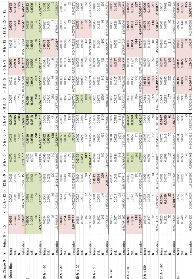
(25) 21. lagged volume change in the previous week before the strategy-formed-day, it is possible to increase the significance of the returns by extending the calculation period for the lagged return and the lagged volume change. In Wang’s Theory (1994), the assumption behind the role of volume is that the market is information asymmetric. Cooper uses previous week and shows results with so many significant returns, which may imply that the private information will not be fully exploited in at least one week. But the private information in Taiwan stock market may exist more than one week, or that. 政治大. influential private information would be fully exploited over one week period.. 立. For that reason, I prolong the calculation period for the lagged return and the. ‧ 國. 學. lagged volume change to two weeks, and the logic of methodology is still the same. Besides, I modify the grid width of price filter to 3%, and 40% for. ‧. high-volume filter, 20% for low-volume filter.. n. C. er. io. al. sit. y. Nat. Return filter. i n U. v. h ethe Table V presents results for i profits are calculated one n gcase c hwhere week after the strategy-formed-day. Those decrease a lot and moderate increase and extreme increase in price in the previous two weeks before the strategy-formed-day have positive returns. Table VI presents results for the case where profits are calculated two weeks after the strategy-formed-day, and the patterns of the returns are different from Table V. The returns with moderate decreases in price has significantly negative return two weeks after the strategy-formed-day, but.

(26) 22. some of which have significantly positive return in Table V still have the same price trend. Table VII and VIII present results for the cases where profits are calculated three and four weeks after the strategy-formed-day. The results in these two tables are remnants of the results for the case where the returns are calculated two weeks after the strategy-formed-day, but some significant results disappear. Additionally, the returns which have extreme increases in. 政治大. the lagged return increase with the elapsed time. Result like Cooper’s still cannot be seen.. 立. ‧ 國. 學. Return and volume filter. ‧. Table V to VIII show an astonishing consistent results with the. y. Nat. io. sit. combination filter of the lagged return and the lagged volume change. In these. a. er. four tables, two regularities are always happened. One is with extreme. n. i vbe negative afterwards. decreases in lagged volumel change, the returns tendnto Another is that when there. Ch. U i e h n c g are increases in both. lagged price and lagged. volume, which is in the fourth quadrant, the returns tend to be positive afterwards. These two regularities are most evident in the case where profits are calculated two weeks after the strategy-formed-day in Table VI. The same observation can also be seen, with less evidence, in Table III, which calculates lagged return and volume change in the previous week before the strategy-formed-day and shows the result for the case where profits are calculated three weeks after the strategy-formed-day..

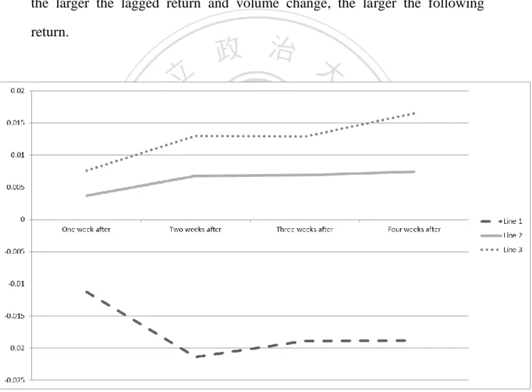
(27) 23. Figure III presents the returns of three two-week filter strategies. Line 1 indicates the average return of filters whose lagged volume changes are smaller than -80%. Line 2 indicates the average return of filters whose lagged returns and volume changes are positive. Line 3 indicate the average return of filters whose lagged returns are larger than or equal to 9% and lagged volume changes are larger than or equal to 80%. From line 2 and 3, we can see that the larger the lagged return and volume change, the larger the following return.. 立. 政治大. ‧. ‧ 國. 學. n. er. io. sit. y. Nat. al. Ch. engchi. i n U. v. Figure III. Return of two-week filter strategy. We may say that there is too much noise in the lagged one week’s return and volume change, or the strength of influential information is not so.

(28) 24. powerful, so the pattern appears random (see Table I) or not so evident afterwards. If using return and volume change in two weeks, the influential information will subdue the noise, or the noise begins to dissipate soon. Also, it seems when lagged return is more extreme, the magnitude of future return tends to be greater. Although the percentage of significant filters increases to 31.67%, and the picture of table seems to be much clearer and less random, again, Wang’s theory (1994) cannot be realized. It is hard to say what happened in the fourth. 治政 quadrant- positive return follows the lagged price 大 and the lagged volume 立 change increase simultaneously- can be the evidence for the theory, because ‧ 國. 學. the results in the other three quadrants is with no relation to the theory. The. ‧. result corresponds more to that found in Gervais, Kaniel, Mingelgrin (2001),. sit. io. er. Nat. but we can see the counterpart.. y. even though we cannot see future price increase with lagged volume increase,. n. a iv IV.4l C Two-day filter n hengchi U. There is another possibility: the market would respond fully to the information at very short time. Thus, I shorten the calculation period for the lagged return and the lagged volume change to only two days. Still, the logic of methodology is the same. Measure two days’ return and volume change to fit in a filter, and then buy the stock at open price on the day just next to the strategy-formed-day. But I modify the grid width of price filter to 1.5%, and 20% for high-volume filter, 12% for low-volume filter. I also change the observation period from 1-4 weeks to two, four, and six days. It is reasonable.

(29) 25. to say that the market would respond fully and faster under this time frame.. Return filter A better result was found this time. Table IX presents results for the case where profits are calculated two days after the strategy-formed-day; Table X four days, and Table XI six days. As can be seen from Table IX to XI, future returns are all significantly. 政治大. positive in negative lagged return filter. Although the return in small lagged. 立. return filter is not economically significant (0.04% in filter of lagged return. ‧ 國. 學. larger or equal to -1.5% and smaller than 0%), the return grows larger when the absolute value of filter becomes larger, and the return also becomes larger. ‧. with time elapsing within 6 days. In positive lagged return filter, the future. y. Nat. io. sit. returns are not all significant, but they still show good outcome. When there is. a. er. an extreme increase in price, the future returns do not tend to be reversed; but. n. v l so extremely, the future when price does not increase n i returns also tends to be Ch. U i e h n c g reversed. The magnitude of future return in positive lagged return filter is not as large as in negative return filter, but we still can see the return grows larger when the absolute value of filter becomes larger, and the return also becomes larger with time elapsing within 6 days (excluding those returns in extreme filter).. Return and volume filter If we examine through Table IX to Table XI, we can see that no matter.

(30) 26. how lagged volume varies, the future returns tend to be reversed. The only difference of the filters between varied volume changes is that in negative lagged volume filter, the return tends to be reversed earlier than in positive lagged volume. We can see that there are more significant filters in negative lagged volume filter than in positive lagged volume filter in Table IX. This phenomenon seems to disappear in the case where profits are calculated four days after the strategy-formed-day in Table X, yet does not disappear completely.. 政治大. Nevertheless, if we just focus on Table IX, we can see that the result has. 立. some similarity with Cooper’s (1999). In Cooper’s result, he compared the. ‧ 國. 學. returns in the combination filter of return and volume change with the returns in the filter of return. He set the return in the return filter as standard. He. ‧. found that the return in the “loser, high-volume” filter is positive but smaller. y. Nat. sit. than the return in the “loser” filter, i.e. the return is reversed rather than. a. er. io. continues. At last, he indicated that his results “support the implications of. n. v l Wang’s (1994) model: winners and losers that experience high growth in ni Ch. U i e h n c g volume in week t-1 tend to experience reduced reversals, and even positive autocorrelation, in week t for winners.” [Cooper (1999, p.919)] If we check my results in this view, we can obtain similar conclusion. The majority of returns in the third and fourth quadrant in Table IX are not significantly different from zero, so we can say that the returns in third quadrant is smaller than in return filter and the returns in fourth quadrant is larger than in return filter. It can also be described that winners and losers experiencing high growth in volume tend to experience reduced reversals, so was shown in.

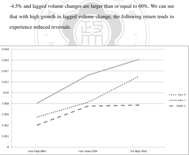
(31) 27. Cooper’s study. Figure IV presents the returns of three two-day filter strategies. Line 1 indicate the average return of filters whose lagged returns are smaller than -4.5% and lagged volume changes are smaller than -36%. Line 2 indicates the average return of filters whose lagged returns are smaller than -4.5% and lagged volume changes are between -12% and -36%. From line 1 and 2, we can see that with moderate decrease in lagged volume change, the following return is greater than that with lots of decrease in lagged volume change. Line. 政治大. 3 indicates the average return of filters whose lagged returns are smaller than. 立. -4.5% and lagged volume changes are larger than or equal to 60%. We can see. ‧ 國. 學. that with high growth in lagged volume change, the following return tends to experience reduced reversals.. ‧. n. er. io. sit. y. Nat. al. Ch. engchi. i n U. v. Figure IV. Return of two-day filter strategy.

(32) 28. At the beginning, I hypothesize, with time, the significant return, positive or negative, will lose its return slowly. However, as duration extends from two days to six days, the magnitude of return does not decrease but increase. It may imply that information needs some time to be fully utilized.. IV.5. Two periods of time. 政治大. Taiwan stock market has developed a lot in these two decades. Taiwan. 立. stock index future and option were launched. Taiwan has also gone through. 學. ‧ 國. Asian financial crisis, the dotcom bubble, and 2007/2008 financial crisis. The fast developing information technology has changed the world noticeably as. ‧. well. Maybe the structure of Taiwan stock market has changed substantially.. Nat. sit er. io. 2003 to 2012.. y. Accordingly, I separate my data into two periods, from 1993 to 2002 and from. n. a. v. i first and second half l C in results betweenn the There are some differences. hengchi U. sample. For example, when there are increases in both return and volume change, the future return tends to be positive in the first half sample, which can be seen in Table XII. However, the phenomenon vanishes in the second half sample, which can be found in Table XIII. Table XII and XIII both present the results for filters where lagged return and lagged volume change are calculated in the previous two weeks. Furthermore, as I calculate lagged return and volume change in two days, the results for the case where profits are calculated two days after the strategy-formed-day are very different, which.

(33) 29. are in Table XIV and Table XV. The returns of “winner, low-volume” and “loser, high-volume” filters tend to be reversed in the second half of the sample, but are not significant in the first half of the sample. In spite of those differences, we still cannot use Wang (1994)’s or Campbell, Grossman, and Wang (1993)’s theory to explain. One certainty is that there is a structure change that makes the returns following the combination of return and volume change to be different.. IV.6. 立. 治政Discussion 大. ‧ 國. 學. In this study, only has some evidence been found to support Wang (1994)’s theory. In his theory, even in an information asymmetric market,. ‧. informed investors can trade for two reasons, private information and liquidity.. y. sit. Nat. On the other hand, a market can sometimes be information asymmetric and. er. io. sometimes be symmetric, because the internal information would not always. n. exist. When the internalainformation diminishes, the i v market is information. l C n U h symmetric. Two kinds of trading e behaviors i place alternately. Sometimes n g c htake trading for private information dominates, and other times trading for liquidity does. Hence the returns for the “loser, high-volume” strategy in Table IX do not continue but experience reduced reversals. Likely, the same reason applies to the other parts of results that are not clear-cut. Two other distinct patterns of return are also been found. One is that in the case where lagged return and volume change are calculated in previous two weeks, a simultaneous increase in lagged return and volume change would be followed by increases in return..

(34) 30. The pattern where the returns experience reduced reversals for the “loser, high-volume” strategy corresponds to Wang’s (1994) theory, but has not been found in the sample of 2003-2012. We conjecture that Taiwan stock market is likely to be more dominated by liquidity trading than by information trading in recent decade. Figure V presents the shareholding ratio of qualified foreign institution investors for three companies- Hon Hai (2317), ASUS (2357), TSMC(2330)which are always on the list of top 50 largest capitalization stocks of listed. 政治大. companies. Qualified foreign institution investors are informed traders. We. 立. can see that their shareholding ratios are higher in 2003-2012 than in. ‧ 國. 學. 1993-2002. Qualified foreign institution investors traded with other noninformed traders when their shareholding ratios are not so high, but traded. ‧. with other qualified foreign institution investors with information in. y. Nat. io. sit. 2003-2012. Relatively, the market in recent decade is symmetric, because the. n. al. er. major investors are all informative. This figure implies the same conjecture. Ch. engchi. i n U. v. Figure V. The shareholding ratio of qualified foreign institution investors.

(35) 31. from the above paragraph. Another distinct pattern found is that returns tend to be negative when lagged volume change decreases extremely. This pattern however may correspond to the predictions of Gervais, Kaniel, Mingelgrin (2001). But we cannot find evidence that stocks experiencing unusual high volume tend to appreciate. It is probably because the windows adopted are different. The level of information asymmetry in market may decrease as the market becomes more and more developed. Cooper’s research is based on. 政治大. samples from 1962 to 1993 that is with information asymmetry. The thesis. 立. looks at data from 1993 to 2013. Although this study and Cooper’s pay. ‧ 國. 學. attention to different markets, these 2 markets have been experiencing the same technology development, such as advancement in information. ‧. technology, internet, and so forth. The U.S. stock market should have changed. y. Nat. io. sit. a lot in these two decades, and the degree of information asymmetry may have. a. er. reduced to great extents. As this thesis demonstrates, the evidence of the. n. iv l existence of information asymmetry becomes less npronounced in the second. Ch. U i e h n c g half of the sampled period, compared to the first half. It suggests reasonably that Taiwan stock market is much more information symmetric. As a result,. the patterns resulted by informed trading become less evident..

(36) 32. Chapter V. Conclusions. The study uses filter rule on Taiwan stock market to investigate the relationship between return and volume change. Some of important. 政治大. observations can be summarized as follows:. 立. First, for a relatively short time window, the lagged return is more. ‧ 國. 學. powerful than the lagged volume change in predicting the return in short-term, and return tends to be reversed. The lagged volume can be a good predictor. ‧. sit. Nat. tends to be negative.. y. for the return when it experiences a substantial decrease. Then, the return. er. io. Second, when the information collecting period extends to two weeks,. n. a return is much more consistent the pattern of the forecast i v with the return of l C n U h previous or next week than that ofeone n gweek. c hIti implies that using filters based. on the lagged return and the volume change in two previous weeks is more powerful to predict the future return than those in previous week. Third, in the case where the filters based on the lagged return and the volume change are calculated in previous two days, when there is low trading volume, the return tends to be reversed; and when there is high trading volume, the return tends to experience reduced reversal. When the calculations are based on information of previous two weeks, simultaneous increases in the lagged return and the volume change tend to be followed by increase in the.

(37) 33. return. These two patterns can be found from the samples spanning 1993-2002, but cannot from the samples spanning 2003-2012. We conjecture that Taiwan stock market is likely to be more dominated by liquidity trading than information trading in recent decade. The pattern of the return for the combination of the lagged return and the volume change is unclear and, sometimes chaotic. This suggests that the evidence found does not correspond to implications of any aforementioned theory perfectly.. 政治大. Conrad, Hameed, and Niden (1994) show that if small capitalization. 立. stocks experience high growth in volume, their returns will display reversal. If. ‧ 國. 學. the stocks experience decreases in volume, a higher chance for continuation in their returns can be observed. Their result yield support for Campbell,. ‧. Grossman and Wang (1993)’s model. Thus, there might be a difference in the. y. Nat. io. sit. relationship in the return and the volume between large and small. a. er. capitalization stocks. A natural way to extend the research is to investigate the. n. v l stocks. But the challenge cases with small capitalization n i of the extension will Ch. U i e h n c g have to deal with the bid-ask bounce problem..

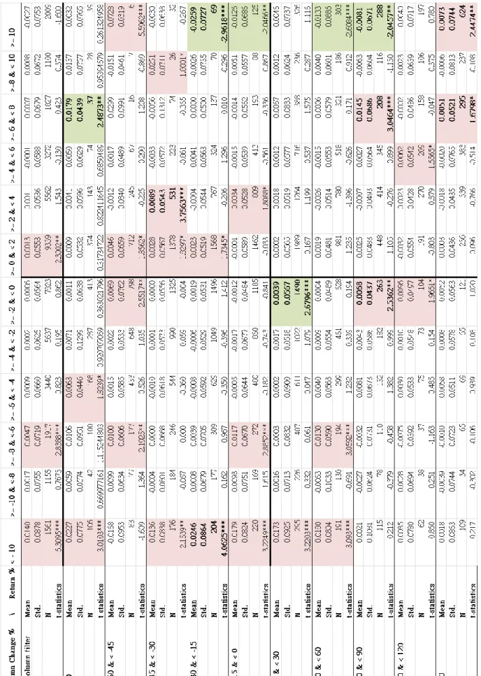
(38) 34. Table I. Results for the case where profits are calculated one week after the strategy-formed-day, and lagged return and volume change are calculated in the previous week, 1993-2012. *,**,*** The null hypothesis is rejected at the 10%, 5%, 1% levels respectively.. 立. 政治大. ‧. ‧ 國. 學. n. er. io. sit. y. Nat. al. Ch. engchi. i n U. v.

(39) 35. Table II. Results for the case where profits are calculated two weeks after the strategy-formed-day, and lagged return and volume change are calculated in the previous week, 1993-2012. *,**,*** The null hypothesis is rejected at the 10%, 5%, 1% levels respectively.. 立. 政治大. ‧. ‧ 國. 學. n. er. io. sit. y. Nat. al. Ch. engchi. i n U. v.

(40) 36. Table III. Results for the case where profits are calculated three weeks after the strategy-formed-day, and lagged return and volume change are calculated in the previous week, 1993-2012. *,**,*** The null hypothesis is rejected at the 10%, 5%, 1% levels respectively.. 立. 政治大. ‧. ‧ 國. 學. n. er. io. sit. y. Nat. al. Ch. engchi. i n U. v.

(41) 37. Table IV. Results for the case where profits are calculated four weeks after the strategy-formed-day, and lagged return and volume change are calculated in the previous week, 1993-2012. *,**,*** The null hypothesis is rejected at the 10%, 5%, 1% levels respectively.. 立. 政治大. ‧. ‧ 國. 學. n. er. io. sit. y. Nat. al. Ch. engchi. i n U. v.

(42) 38. Table V. Results for the case where profits are calculated one week after the strategy-formed-day, and lagged return and volume change are calculated in the previous two weeks, 1993-2012. *,**,*** The null hypothesis is rejected at the 10%, 5%, 1% levels respectively.. 立. 政治大. ‧. ‧ 國. 學. n. er. io. sit. y. Nat. al. Ch. engchi. i n U. v.

(43) 39. Table VI. Results for the case where profits are calculated two weeks after the strategy-formed-day, and lagged return and volume change are calculated in the previous two weeks, 1993-2012. *,**,*** The null hypothesis is rejected at the 10%, 5%, 1% levels respectively.. 立. 政治大. ‧. ‧ 國. 學. n. er. io. sit. y. Nat. al. Ch. engchi. i n U. v.

(44) 40. Table VII. Results for the case where profits are calculated three weeks after the strategy-formed-day,. and lagged return and volume change are calculated in the previous two weeks, 1993-2012 *,**,*** The null hypothesis is rejected at the 10%, 5%, 1% levels respectively.. 立. 政治大. ‧. ‧ 國. 學. n. er. io. sit. y. Nat. al. Ch. engchi. i n U. v.

(45) 41. Table VIII. Results for the case where profits are calculated four weeks after the strategy-formed-day,. and lagged return and volume change are calculated in the previous two weeks, 1993-2012 *,**,*** The null hypothesis is rejected at the 10%, 5%, 1% levels respectively.. 立. 政治大. ‧. ‧ 國. 學. n. er. io. sit. y. Nat. al. Ch. engchi. i n U. v.

(46) 42. Table IX. Results for the case where profits are calculated two days after the strategy-formed-day, and lagged return and volume change are calculated in the previous two days, 1993-2012. *,**,*** The null hypothesis is rejected at the 10%, 5%, 1% levels respectively.. 立. 政治大. ‧. ‧ 國. 學. n. er. io. sit. y. Nat. al. Ch. engchi. i n U. v.

(47) 43. Table X. Results for the case where profits are calculated four days after the strategy-formed-day, and lagged return and volume change are calculated in the previous two days, 1993-2012. *,**,*** The null hypothesis is rejected at the 10%, 5%, 1% levels respectively.. 立. 政治大. ‧. ‧ 國. 學. n. er. io. sit. y. Nat. al. Ch. engchi. i n U. v.

(48) 44. Table XI. Results for the case where profits are calculated six days after the strategy-formed-day, and. lagged return and volume change are calculated in the previous two days, 1993-2012 *,**,*** The null hypothesis is rejected at the 10%, 5%, 1% levels respectively.. 立. 政治大. ‧. ‧ 國. 學. n. er. io. sit. y. Nat. al. Ch. engchi. i n U. v.

(49) 45. Table XII Results for the case where profits are calculated two weeks after the strategy-formed-day, and lagged return and volume change are calculated in the previous two weeks, 1993-2002 *,**,*** The null hypothesis is rejected at the 10%, 5%, 1% levels respectively.. 立. 政治大. ‧. ‧ 國. 學. n. er. io. sit. y. Nat. al. Ch. engchi. i n U. v.

(50) 46. Table XIII Results for the case where profits are calculated two weeks after the strategy-formed-day, and lagged return and volume change are calculated in the previous two weeks, 2003-2012 *,**,*** The null hypothesis is rejected at the 10%, 5%, 1% levels respectively.. 立. 政治大. ‧. ‧ 國. 學. n. er. io. sit. y. Nat. al. Ch. engchi. i n U. v.

(51) 47. Table XIV Results for the case where profits are calculated two days after the strategy-formed-day, and lagged return and volume change are calculated in the previous two days, 1993-2002 *,**,*** The null hypothesis is rejected at the 10%, 5%, 1% levels respectively.. 立. 政治大. ‧. ‧ 國. 學. n. er. io. sit. y. Nat. al. Ch. engchi. i n U. v.

(52) 48. Table XV Results for the case where profits are calculated two days after the strategy-formed-day, and lagged return and volume change are calculated in the previous two days, 2003-2012 *,**,*** The null hypothesis is rejected at the 10%, 5%, 1% levels respectively.. 立. 政治大. ‧. ‧ 國. 學. n. er. io. sit. y. Nat. al. Ch. engchi. i n U. v.

(53) 49. Reference Blume, Lawrence; Easley, David; and O’Hara, Maureen, 1994, Market-Statistics and Technical Analysis: The Role of Volume, Journal of Finance, 49, 153-181. Campbell, John Y.; Grossman, Sanford J.; and Wang, Jiang, 1993, Trading Volume and Serial Correlation in Stock Returns, Quarterly Journal of Economics, 108, 905-939. Chen, Yi-Yuan, 2006, A Study on Volume and Price Relationship in the Taiwan Stock Index- by the Method of Filter Rule, Unpublished Master Thesis, National Taipei University. (In Chinese). 政治大. Conrad, Jennifer S.; Hameed, Allaudeen; Niden, Cathy, 1994, Volume and Autocovariances in Short-Horizon Individual Security Returns, Journal of Finance, 49, 1305-1329. 立. Cooper, Michael, 1999, Filter Rules Based on Price and Volume in Individual Security. ‧ 國. 學. Overreaction, Review of Financial Studies, 12, 901-935.. ‧. Gervais, Simon; Kaniel, Ron; and Mingelgrin, Dan H., 2001, The High-Volume Return Premium, Journal of Finance, 56, 877-919.. y. Nat. sit. Hsu, Shih-Shang, 2004, Market Efficiency of Taiwan Index Futures Market- Filter Rule. n. al. er. io. Approach, Unpublished Master Thesis, National Chengchi University (In Chinese). Ch. i n U. v. Kelley, Eric Kyle, 2004, Evidence to the Contrary: Extreme Weekly Returns are Underreactions,. engchi. Unpublished Doctoral Dissertation, Texas A&M University. Lehmann, Bruce N., 1990, Fads, Martingales, and Market Efficiency, Quarterly Journal of Economics, 105, 1-28. Mayshar, Joram, 1983, On Divergence of Opinion and Imperfections in Capital Markets, American Economic Review, 73, 114–128. Miller, Edward M., 1977, Risk, Uncertainty, and Divergence of Opinion, Journal of Finance, 32, 1151–1168. Wang, Jiang, 1994, A Model of Competitive Stock Trading Volume, Journal of Political Economy, 102, 127-168.

(54)