一個使用手機網路資料預估交通路況的演算法系統

國 立 交 通 大 學

網路工程研究所

碩 士 論 文

一個使用手機網路資料預估交通路況的演算法系統

A Traffic Estimation Algorithm Using Cellular Network Data

研 究 生：賴岳廷

指導教授：張明峰 教授

一個使用手機網路資料預估交通路況的演算法系統

A Traffic Estimation Algorithm Using Cellular Network Data

研 究 生：賴 岳 廷 Student: Yueh-Ting Lai

指導教授：張 明 峰 Advisor: Ming-Feng Chang

國立交通大學 網路工程研究所

碩士論文

A Thesis

Submitted to Institute of Network Engineering College of Computer Science

National Chiao Tung University in Partial Fulfillment of the Requirements

for the Degree of Master

In

Computer Science June 2010

Hsinchu, Taiwan, Republic of China

一個使用手機網路資料預估交通路況的演算法系統

研究生：賴岳廷

指導教授：張明峰 老師

國立交通大學網路工程研究所

摘要

即時交通資訊服務系統的建置屬於智慧型運輸系統(Intelligent Transportation System, ITS)重要的一環，對於用路人而言，獲得完整且充足的交通資訊，不論 是行前路況資訊以及行進中的路況資訊，大眾運輸轉乘資訊等等，都能提供用路 人在不同路徑以及運具的選擇上，具有更加的彈性。 近年來，隨著科技的發展，手機已經廣泛為大眾所使用，有鑑於此，我們將 利用手機的換手(Handover)行為，求出道路中行進手機換手位置，並利用無線電 信網路追蹤使用者手機位置的方式，產生即時道路交通路況資訊。這個機制不需 要花費龐大的經費來架設及維護道路上的車輛偵測裝置(Stationary Vehicle Detector (SVD).)。而且手機幾乎是無所不在的，因此我們以追蹤手機位置所得到 的交通資訊是非常即時且全面的。不過在研究當中，我們發現在擁塞的交通路況 下，手機使用者因為移動的限制造成過少甚至沒有換手的行為發生，以至於此種 機制在擁塞的交通條件下無法準確的評估交通路況。因此我提出了利用手機來電 (Call Arrival)與掛斷(Call Complete)的行為，配合車輛偵測裝置的歷史資料來預測 交通密度。結合了這兩者的機制，設計出一個能利用電信業者網路端的手機資訊 來評估完整交通路況的方法，來達到對於擁塞的交通狀況更準確的預測。

A Traffic Estimation Algorithm Using Cellular Network Data

Student: Yueh-Ting Lai

Advisor: Dr. Ming-Feng Chang

Institute of Network Engineering

Nation Chiao Tung University

Abstract

The construction of real-time traffic information service is an important part of Intelligent Transportation System (ITS). For a road user, knowing real-time traffic information would help him in choosing better roads avoid congestion areas. ITS has become more and more popular in recent years. Traffic monitoring based on cellular network data can be more cost-effective, traditional approaches, such as roadside sensors, because no field installation or maintenance is needed. Double handover events from the Cellular Floating Vehicle Data (CFVD) can be used to estimate traffic speed. However, when the traffic is congested, due to the slow movements of the traffic, there could be very double handover events and thus very few effective speed reports of CFVD. In this paper, we propose a novel algorithm that studies the relationship between call arrival rate, call complete rate and the traffic density to estimate the traffic conditions. In addition, we combine this mechanism with the CFVD to estimate the traffic speed, especially in the condition of traffic congestion, with more accuracy and real-timeliness. Computer simulations have also been conducted to evaluate the effectiveness of our algorithm.

誌謝

首先我要感謝的是我的論文指導老師 張明峰教授，在碩士班這兩年的求學 生涯中，老師有耐心的督促和指導、訓練獨立思考和研究能力，並細心地從我的 研究當中發掘問題，一步一步指引我完成論文。也感謝老師也提供了完善的實驗 室環境和硬體資源，使學生能專注於研究不受限制，再次謝謝老師兩年來的教 誨。 再來我要特別感謝實驗室博士班學長陳志華，在我的論文研究期間協助我克 服研究中所遇到的困難和盲點，並給予了我很多研究方法和建議。也要感謝我的 實驗室學長玄亞、威凱和柏瑞，同學祐村和茂弘，學弟順胤和境余，在我研究所 求學的兩年當中一起修課、討論課業和互相勉勵，使我這段時間在生活上增添了 許多的色彩。 最後我要將此論文獻給我最親愛的家人，感謝您們在我求學期間全心全意的 支持，讓我得以順利地完成學業。 賴岳廷 謹識於 國立交通大學網路工程研究所碩士班 中華民國九十九年九月

Contents 摘要 ... i Abstract ... ii 誌謝 ...iii List of Figures ... vi Chpater 1 Introduction ... 1 1.1 Motivation ... 1 1.2 Traffic Information ... 1 1.3 Objective ... 3 1.4 Summary ... 4

Chpater 2 Related Works ... 5

2.1 The Architecture of GSM and UMTS ... 5

2.2 Handover Concept ... 6

2.3 Speed and Travel Time ... 8

2.4 Traffic Flow ... 9

2.5 Accidents ... 10

2.6 Summary ... 11

Chpater 3 System Design and Algorithms ... 12

3.1 Speed Estimation by Handover Events ... 12

3.2 TMS, SMS and Three-phase Traffic theory ... 13

3.3 The Basic Idea of Our Algorithms ... 15

3.4 The estimation of N ... 16

3.5 Traffic State Determination Algorithm ... 17

3.6 Correction from SMS to TMS ... 19

3.7 Vehicle Speed Estimation from N ... 22

3.8 Our System design and Algorithms ... 24

4.1 Simulation Environment ... 26

4.2 Simulation Results ... 28

Chpater 5 Conclusion and Future Work ... 34

List of Figures

FIGURE 2-1THE ARCHITECTURE OF GSM NETWORK... 5

FIGURE 2-2THE ARCHITECTURE OF COMBINED GSM AND UMTS NETWORK ... 6

FIGURE 2-3THE DIAGRAM OF BASE STATION, CELL AND HANDOVER. ... 8

FIGURE 2-4THE CELLULAR EVENT COUNTS IN A WEEK [10] ... 10

FIGURE 2-5THE ANOMALY OF CELLULAR EVENT COUNTS IN A WEEK [10] ... 11

FIGURE 3-1THE CELL SWITCHING OF A MOVING MS ALONG A ROAD ... 12

FIGURE 3-2THE SCHEMATIC DIAGRAM OF TMS AND SMS ... 13

FIGURE 3-3THE SPEEDS OBTAINED FROM VD AND FROM GPS PROBE CARS ... 14

FIGURE 3-4THE RELATION OF THE INFORMATION IN OUR SIMULATION ... 15

FIGURE 3-5THE EXAMPLE OF POWER LAW FOR CORRECTION ... 22

FIGURE 3-6THE EXAMPLE OF POWER LAW FOR SPEED ESTIMATION ... 24

FIGURE 3-7THE FLOW CHART OF OUR SYSTEM DESIGN AND ALGORITHMS ... 24

FIGURE 4-1THE CONCEPT OF OUR SIMULATION ... 26

FIGURE 4-2THE DIAGRAM OF HOS AND ACCIDENT ON THE ROAD SEGMENT ... 28

FIGURE 4-3THE INFORMATION OF THE BEST RESULT IN OUR SIMULATION ... 31

FIGURE 4-4THE BEST RESULT OF SPEED ESTIMATION IN OUR SIMULATION ... 31

FIGURE 4-5THE INFORMATION OF THE WORST RESULT IN OUR SIMULATION ... 32

FIGURE 4-6THE WORST RESULT OF SPEED ESTIMATION IN OUR SIMULATION ... 32

FIGURE 4-7THE INFORMATION OF THE AVERAGE RESULT IN OUR SIMULATION ... 33

List of Tables

TABLE 3-1THE PARAMETERS FOR ESTIMATING VEHICLE SPEED ... 16

TABLE 3-2THE PARAMETERS OF STATE DETERMINATION ALGORITHM ... 17

TABLE 3-3THE PARAMETERS OF LINEAR REGRESSION FOR CORRECTION ... 20

TABLE 3-4THE PARAMETERS OF POWER LAW FOR CORRECTION ... 21

TABLE 3-5THE PARAMETERS OF LINEAR REGRESSION FOR SPEED ESTIMATION ... 22

TABLE 3-6THE PARAMETERS OF POWER LAW FOR SPEED ESTIMATION FROM N ... 23

TABLE 4-1THE SIMULATION SET UP AND PARAMETERS OF OUR SIMULATION ... 27

TABLE 4-2THE OVERALL ERROR RATIO OF OUR SPEED ESTIMATION ALGORITHM ... 29

TABLE 4-3THE HIT RATIO OF OUR STATE DETERMINATION ALGORITHM ... 30

Chpater 1

Introduction

1.1 Motivation

With the development of the technology, traffic information has become more

and more important for saving time in our busy life. Hence, there is an increasing

need to construct the Intelligent Transportation System (ITS). The ITS can provide

real-time traffic information such as traffic speed, flow, travel time, and accident

events to the road users and traffic managers. Real-time traffic information will be

helpful to road users in choosing better roads to avoid congested areas. This

information can be also used to support vehicle dispatch system, on-vehicle

navigation system, and traffic control. Thus real-time traffic information will improve

the level of services of roadways.

1.2 Traffic Information

There are three typical approaches in collecting the real-time traffic information: (1) Vehicle Detector (VD)

(2) Global Position System (GPS)-based probe cars

(3) Cellular Floating Vehicle Data (CFVD).

Vehicle Detector (VD), such as inductive loop detectors and video image

processors, are installed on the side of roads and bridges [1, 2]. VDs detect the instant vehicle’s speed and calculate the traffic flows when a vehicle moves across the

detection area. Although this approach can provide the real-time and accurate traffic

information, it costs a lot to purchase and install these VDs. Moreover, the

maintenance cost is also high because of the high failure rates of VDs caused by the

climate factors such as high temperature, or wet weather [1], or even natural disasters

such as typhoons. Therefore, using VDs to construct a wide-area ITS needs a large

amount of money for installation and maintenance.

With Global Position System (GPS)-based probe cars, traffic information is

collected from the probe cars equipped with GPS receivers and wireless

communication devices. The GPS-based probe cars record and provide the central

information server their locations and speeds; the central information server collects

and processes the information then broadcasts it to the cars on the roadways

periodically [1, 2]. However, due to the limited number of probe cars, the amount of

collected data is usually not enough to infer the real-time traffic information.

In the Cellular Floating Vehicle Data (CFVD) approach, traffic information is

obtained from the anonymously sampling locations of the Mobile Station (MS) [3-9].

When a communicating MS is moving away from the area covered by one cell and

entering the area covered by another cell, it performs the handover procedure.

Furthermore, the cellular core network will record the location of MS and timestamp

events to estimate the MS’s speed from the time difference and the distance between

these two handover records. Therefore, the CFVD approach does not require a huge

amount of money to install or maintain additional devices. Since cell phone has been

widely used nowadays, the traffic information obtained from CFVD is

comprehensive.

1.3 Objective

As we have mentioned, CFVD have the advantages of low cost and

comprehensive coverage, but CFVD still have some drawbacks. In the condition of

traffic congestion, due to the slow movements of the traffic, handover events during

the congestion period are rare until the congestion is released, i.e., CFVD is able to

react to the condition of traffic congestion. Traffic information system that can not

inform road users of congestion condition is meaningless. Moreover, the average

speed and travel time inferred from CFVD are more realistic than those obtained from

VDs, because VDs record the instantaneous speeds and estimate the travel time by the

space-mean speed, which CFVD observes travel time directly. So in this paper, we

1.4 Summary

The remaining part is organized as following. Chapter 2 describes the system

architectures of Global System for Mobile Communications (GSM) and Universal

Mobile Telecommunications System (UMTs) cellular network, and introduces the

related work of CFVD. Chapter 3 presents our algorithms and system design. Chapter

4 shows the simulations results and performance of our system. Finally, we will

Chpater 2 Related Works

GSM and UMTS are the most popular standards for cellular communication. Hence, the researchers generally use these two standards to develop the CFVD systems. We will briefly describe the GSM, UMTS and handover procedure since handover events are used to infer the traffic information.

2.1 The Architecture of GSM and UMTS

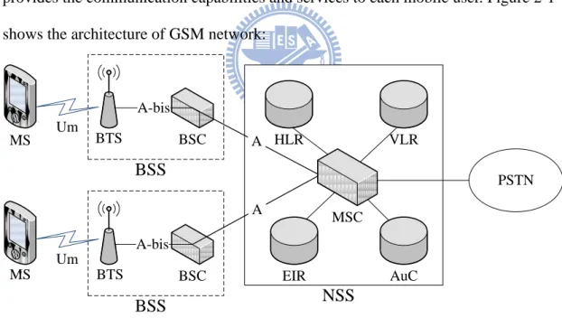
Global System for Mobile Communications (GSM) is the widely used 2nd

Generation standard for mobile communication systems in the world, which is innovated by European Telecommunications Standardization Institute (ETSI).It provides the communication capabilities and services to each mobile user. Figure 2-1 shows the architecture of GSM network:

v v MS MS BTS BTS Um Um BSC BSC A-bis A-bis BSS BSS HLR AuC VLR EIR MSC NSS A A PSTN

Figure 2-1 The architecture of GSM network

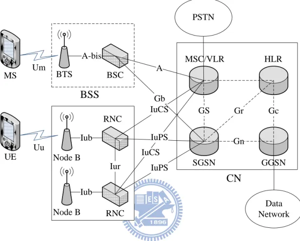
Universal Mobile Telecommunications System (UMTS) is one of third generation (3G) mobile technology which evolved from the GSM. It provides high-bandwidth data and voice services to mobile users, such as text, digital voice, video, and multimedia. The UMTS is specified by 3rd Generation Partnership

Project (3GPP). Figure 2-2 shows the architecture of combined GSM and UMTS network: v v MS UE BTS Node B Um Uu BSC A-bis

BSS

GGSN SGSN

CN

PSTN Node B RNC Iub Iub Iur RNC GS Gc Gn Gr MSC/VLR HLR IuCS A Gb IuPS IuPS IuCS Data Network

Figure 2-2 The architecture of combined GSM and UMTS network

2.2 Handover Concept

The handover will occur when there is a need for cell change during a call. The handover procedure moves the control of the call session from one base station (the BTS in GSM and Node B in UMTS depicted above) to another. There are three basic types of handovers:

(1) Hard Handover

The definition of hard handover is that the link between the MS and the old BS should be broken before a new one with the new BS is established. There is a short

not notice.

(2) Soft Handover

The type of handover is that MS can communicate with more than one base station or Node B during the handover procedure. It will provide a more reliable and seamless handover procedure. In UMTS, most of handovers are performed using this type.

(3) Softer Handover

The softer handover is that MS can communicate with more than one sector of the same Node B. It will occur when a MS can detect signals from two sectors of the same Node B, and the radio links that are added to and removed from the same Node B. This type of handover is available in UMTS.

The handovers of GSM are hard handovers, and hard handovers can also be distinguished into three types: Intra-BSC Handover, Inter-BSC Handover and Inter-MSC Handover depending on the network structure.

In UMTS, due to the advent of CDMA technology, it provides a more reliable and seamlessly handover. As a result, these three different forms of handover are all available for UMTS depending on different circumstances.

The soft and softer handover may cause the handover behavior more complex because the multiple links to the base station. We have been analyzed some real database of handover behavior from telecommunication company, the results showed that the database of GSM are more certain in distinguishing the handover pairs and handover location than the UMTS. But due to the limited amount of data, we can’t conclude that the hard handover is better than the soft handover in CFVD, we will do furthermore analysis of them in the future. Then we describe the concept of the base station, cell and handover events for CFVD.

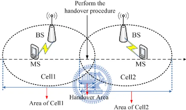
number of Base Stations (BSs). Without loss of generality, the radio coverage of a BS is called a cell. Each cellhas a unique identity called Cell Global Identification (CGI). When a Mobile Station (MS) attaches to the cellular network, it will be served by a BS and store the BS’s CGI.If a communicating MS moves from one BS to another, the MS will perform handover procedure.Figure 2-3 shows the diagram of base station, cell and handover.

Figure 2-3 The diagram of base station, cell and handover.

2.3 Speed and Travel Time

Since the area where handovers may occur is significantly smaller than the coverage area of a base station, when a call performs the handover procedure, the location of the MS can be located with a higher accuracy (Figure 2-3). Hence, the mostly used signalings for speed and travel time estimation are handover events of GSM and UMTS. Sven Maerivoet and Steven Logghe [3] showed that CFVD is capable of detecting congestion during the morning and evening rush hours, and they also indicated that CFVD has a better coverage than traditional VDs on the roadside

of the road network and its performance on the highway environment is very good. Their results showed that the relative error between CFVD and the travel time obtained from GPS probe cars on the highway environment is less than 15% for over 70% to even 90% of the road segments. Hence, the CFVD has potential that it can provide complete traffic information of the road network. Hillel [4] evaluated CFVD along the Ayalon freeway in the ISRAEL, he found that the CFVD was more noisy than loop detectors. In the measurement of consecutive 5 min intervals on the same road section, he showed the average absolute relative difference between travel time data is 14% for CFVD and 4% for loop detectors. Overall, he concluded that the correspondence between CFVD and loop detectors was generally good, and it was suitable to use in the practical traffic environment. Gundlegard and Karlsson [7] showed that high accuracy in localizing the handover locations can be obtained from both the GSM and UMTS. Their results showed the traffic speed estimation is more accurate in UMTS than in GSM. They also indicated that using signaling data of GSM to estimate traffic information on highways is promising. Moreover, by combine the signaling of GSM and UMTS to extend the coverage for CFVD, it may be possible for usage in the urban environments.

2.4 Traffic Flow

In the measurement of traffic flow using CFVD, one can count the amount of signaling data of Cellular Network along a road. It is possible to use the signaling data to infer the traffic flow or estimated traffic condition. Danilo Valerio [10] used Cell updates (handover), Location Area Update, Routing Area Update and Combine RAU and LAU to roughly estimate the traffic condition in the Sud-Autobahn between Vienna and Wiener Neustadt. His results indicated that the data obtained from the cellular network can depict the peak traffic time and the difference between working

days and weekend days is clear. Figure 2-4 shows an example of the total cellular events in a week from their system [10]. In the working days, the peaks of event counts are located at the busy hours 7:00-8:00 and 16:00-17:00, and in weekend days, the peaks of event counts are located at near 9:00-10:00.

Figure 2-4 The cellular event counts in a week [10]

2.5 Accidents

The main approaches to detect the accidents using CFVD are anomalies of cellular network data. One can analyze the long term historical data of cellular network, such as the counts of handover events, the counts of RAU and LAU events in any period of time to establish the historical databases of a specific road segment, and compare the real-time cellular network data with the historical database to check the unusual pattern to infer possible accident cases. Danilo Valerio [10] observed the pattern of the number of combined RAU and LAU events. He found that the abrupt changes, such as a notch immediately followed by a peak from the pattern, are caused

Busy hours at 16:00 – 17:00 Busy hours at 7:00 – 8:00 Busy hours at 9:00-10:00

can’t perform the RAU and LAU procedures. When the accident is removed, a large number of cars may move across the boundary of LA or RA and perform LAU or RAU in short time period. Figure 2-5 shows the anomaly of cellular event counts combined RAU and LAU in a week [10].

Figure 2-5 The anomaly of cellular event counts in a week [10]

2.6 Summary

There are some drawbacks of these related works using CFVD. In the aspect of speed and travel time, since handover events during the congestion period are rare until the congestion is released, CFVD system can’t offer the speed and travel time in the condition of traffic congestion. About the LAU, RAU event counts for traffic flow and accident detection, due to the less accurate localization of LAU and RAU, the estimation may impacted by unpredictable factors. Moreover, the anomaly of cellular event counts is really hard to define. Hence, in Chapter 3 we will overcome these drawbacks and propose a novel system to estimate the traffic condition more accurately.

Chpater 3 System Design and Algorithms

In this chapter, first we introduce how the speed is estimated by the handover events, and then describe the concept of Time Mean Speed (TMS), Space Mean Speed (SMS) and three-phase traffic theory. From the results of our computer simulations, we propose our system design and algorithms.

3.1 Speed Estimation by Handover Events

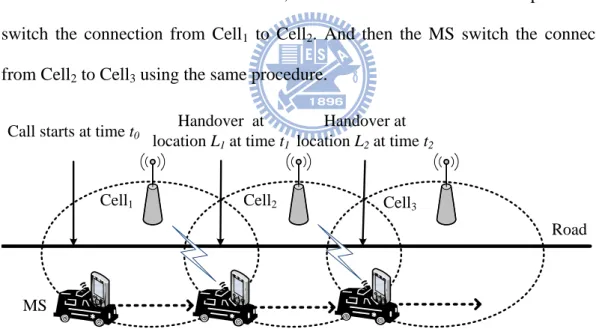
Figure 3-1 shows how we use handover records to infer the traffic speeds. A communicating MS in a car moves along the road and is connected to Cell1 at time t0.

When the MS enters the coverage of the Cell2 at t1 and the radio signal strength from

the new BS is better than the old BS, the MS executes the handover procedure to switch the connection from Cell1 to Cell2. And then the MS switch the connection from Cell2 to Cell3 using the same procedure.

Cell1 Handover at location L1 at time t1 Handover at location L2 at time t2 Road Cell2 Cell3

Call starts at time t0

MS

v v v

Figure 3-1 The Cell Switching of a moving MS along a road

The speed of the MS can be estimated by using two consecutive standard handover procedures described above. When the MS changes the connection to a new BS, it obtains the BS’s CGI. Therefore, from the two consecutive handovers depicted in figure 3-1, we can obtain the handover pair (CGI , CGI) for the first handover at

time t1 and handover pair (CGI2, CGI3) for the second handover at time t2. If we can

estimate the location (L1, L2) of handover pair (CGI1, CGI2) and handover pair (CGI2,

CGI3), then we can estimate the speed of the MS as

_

_

1 2 2 1 t t L L v   in the period [t1, t2],

where d(L₁,L₂)denotes the distance on the road between L1 and L2.

3.2 TMS, SMS and Three-phase Traffic theory

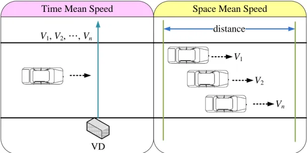
TMS is the average speed of vehicles passing a specific point on a road during a period of time. SMS is the average speed of vehicles passing a specific road segment during an interval of time. There are many researches about the TMS and SMS in the transportation engineering [11-12]. In the researches on the relation between TMS and SMS, TMS is always higher than the SMS. By the definition of TMS and SMS, the speed obtained from GPS probe car is SMS and from VD is TMS. Figure 3.2 shows the schematic diagram of TMS and SMS.

Time Mean Speed Space Mean Speed

VD distance V1, V2, …, Vn V1 V2 Vn

Figure 3-2 The schematic diagram of TMS and SMS

of three-phase traffic theory. He focuses mainly on the explanation of the physics of traffic breakdown and resulting in congested traffic on highways. Kerner describes three phases of traffic, while the classical theories based on the fundamental diagram of traffic flow have two phases: free flow and congested traffic. Hence, Traffic consists of free flow and congested traffic, and the congested traffic consists of two traffic phases. Thus, there are three traffic phases:

(1) Free flow.

(2) Synchronized flow. (3) Wide moving jam.

In our simulations, we set the VDs on the road every 250m to derive the average instantaneous speeds of cars between two handover points, and simulate the GPS probe cars to derive the speeds by calculating the time difference and distance between two handover points. We observe that in the condition of traffic congestion (synchronized flow and wide moving jams), and the speed obtained from GPS probe cars (i.e., SMS) is slower than the speed obtained from VD (i.e., TMS) as shown in Figure 3-3.

Figure 3-3 The speeds obtained from VD (TMS) and from GPS probe cars (SMS)

0 10 20 30 40 50 60 70 80 90 100 900 1500 2100 2700 3300 3900 4500 5100 5700 6300 6900 7500 8100 Sp e e d (k m /h ) Simulation Time(s) VD GPS

3.3 The Basic Idea of Our Algorithms

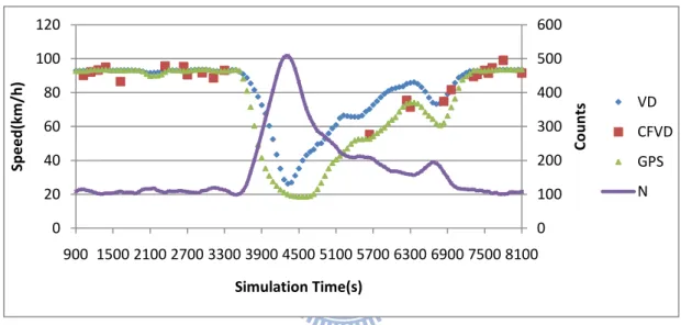
Let N denote the number of cars in the road segment under consideration; N can be also considered as the traffic density. Figure 3-4 depicts our simulation results about the relation of CFVD reports, N, and speed obtained from GPS probe cars and VDs. There are few effective reports of CFVD in the condition of traffic congestion. However, we also find the negative correlation between the speed of VDs and the number of cars in the road segment covered by the specific cell.

Figure 3-4 The relation of the information in our simulation

Hence, the basic idea of our algorithm is using the speed of CFVD report if it exists, else we will utilize the N to infer the traffic speeds. However, for the purpose of evaluating the accuracy of the speed obtained from CFVD with the VD set up on the road, and due to the difference between TMS and SMS described in Section 3.2, the speeds of CFVD (SMS) reports need to be corrected to match the speeds of VDs (TMS). Hence we propose an algorithm to separate the traffic condition to free flow and the congested flow (i.e., synchronized flow and wide moving jams of three-phase traffic theory). In Section 3.4 and 3.5, we will present the estimation of the number (N) of cars in the road segment covered by the specific cell and the traffic state

0 100 200 300 400 500 600 0 20 40 60 80 100 120 900 1500 2100 2700 3300 3900 4500 5100 5700 6300 6900 7500 8100 Co u n ts Sp e e d (k m /h ) Simulation Time(s) VD CFVD GPS N

determination algorithm. Then we will describe how we correct the CFVD (SMS) speed to match the VD (TMS) speed and derive estimated speed from N in Sections 3.6 and 3.7.

3.4 The estimation of N

We define some parameters for estimating vehicle speeds in Table 3-1. Table 3-1 The parameters for estimating vehicle speed

N

The number of cars in the road segment covered by the specific cell

R

ca The new call arrival rate in the specific cell

R

cc The call completion rate in the specific cell



The call arrival rate

1/



The average call holding time

C

The number of communicating calls in the segment covered by the specific cell

We also make some assumptions to simplify the estimation of vehicle speeds: (1) We only consider the MS of moving vehicles on the road.

(2) The call arrival process is Poisson process with rate 

(3) The call holding time is exponentially distributed with mean 1/

By the definition of parameters, we can deduce the following equations:

   N R_ca             C N N R_cc

Since R_cc  R_ca  N  from the two equations described above, we can conclude that the estimated N is equal to

     2 ca cc cc R R R

. Hence, we can use the new call arrival rate and call completion rate in the specific cell to estimate N which can be utilized to infer the vehicle speed.

3.5 Traffic State Determination Algorithm

For the purpose to separate traffic conditions to free flow and congested flow described in Section 3.3, we purpose the traffic state determination algorithm in this section. First we define some parameters of the algorithm in Table 3-2.

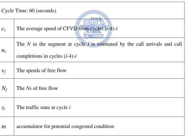
Table 3-2 The parameters of state determination algorithm Cycle Time: 60 (seconds)

c

i The average speed of CFVD from cycles (i-4)-i

n

i

The N in the segment at cycle i is estimated by the call arrivals and call completions in cycles (i-4)-i

v

f The speeds of free flow

N

f The Ns of free flow

s

i The traffic state at cycle i

m

accumulator for potential congested condition

The state determination algorithm consists of two parts: (1) free to jam algorithm and (2) jam to free algorithm.

I. Free to jam algorithm

 





 





if end else then if if end else 1 then if else 1 then exists if : Jam) to (Free Algorithm 1 2 2 1 1 1 0 2 0 1 . 0 1 . 0 max min 9 . 0                             i i i i i i i i i f i f i i s s jam s m m m m m n n n and n n n or N n m m v c and c

II. Jam to free algorithm

if end lse e then exists if : Free) to (Jam Algorithm 1 ) max( ) min(      i i i f i f i i s s free s N n and v c and c

The system starts at state of free flow. When the system is in the state of free flow, it only executes the free to jam algorithm every cycle time to check whether the state should be changed. If the system is in the state of congested flow, it only executes the jam to free algorithm every cycle time to check whether the state should

be recovered to the free flow.

In the part of jam to free algorithm, if the system satisfies all the following conditions at cycle i, it will change the state from congested flow to free flow.

(1) CFVD reports exist during cycle (i-4)-i

(2) The report speed is equal or greater than the minimum speed of free flow

(3) The estimated N from call arrivals and call completions of cycle (i-4)-i is smaller than the maximum Ns of free flow

In the free to jam algorithm, we will set an accumulator for potential congested condition (m), if the system satisfies the following condition twice consecutively at cycle i, it will set the state from free flow to congested flow.

(1) CFVD reports exist during cycle (i-4)-i, but the average of report speeds is smaller than 90% of minimum speed of free flow.

(2) No CFVD reports during cycle (i-4)-i and the estimated N from call arrivals and call completions of cycle (i-4)-i is greater than maximum Ns of free flow.

(3) No CFVD reports during cycle (i-4)-i and the ni, ni-1 are greater than 110% of ni-1, ni-2 respectively.

The state determination algorithm is flexible for different road segments, the factor of 90%, 110% and the parameter of algorithm can be modified to fit different road environment.

3.6 Correction from SMS to TMS

As described in Section 3.3, we want to correct the CFVD (SMS) speed to match the VD (TMS) speed for evaluation of the system. We use the historical data of GPS probe cars and VD data as training data to infer the equation between them, and use

this equation for correction. There are two main approaches we use to find the equation:

(1) Linear Regression(LR)

The linear regression is the statistic approaches used to analysis the relationship between two variables in the form of linear equation. First we define the parameters of linear regression for correction from SMS to TMS in Table 3-3.

Table 3-3 The parameters of linear regression for correction

The average SMS obtained from GPS records from cycles (i-4)-i

The average TMS obtained from VD from cycles (i-4)-i

c

i The average speed of CFVD from cycles (i-4)-i

Then we can use the formula of linear regression to infer TMS of its

corresponding speed of CFVD report as

v

i





c

i









Where xx xy

S

S





ˆ

and k x i k y k i k i i





  _  1  1  











                           k i k i k i i i xx k i i k i i i i xy k x x k y x y x

_S

S

1 1 2 1 2 1 1 , (2) Power Law (PL)

The power law is one of the mathematical relationship between two variables,

i

x

i

the number of one variables Y varies as a power of another variable X, we said the

Y follows a power law. We define the parameters of power law for correction from

SMS to TMS in Table 3-4.

Table 3-4 The parameters of power law for correction

x

min The minimum speed of

y

xmin The speed of when

y

max The maximum speed of

x

ymax The speed of when



The adjusted parameter

And we can infer TMS of its corresponding speed of CFVD report as



_{max min}



_min

min max min x x y i i

y

y

y

x

x

x

c

v

_





























The concept of the power law is to set two boundary coordinates, in this formula they are (

x

min

, y

xmin) and (

x

ymax

, y

max), and compare

c

i with these two

coordinates to determine the estimated TMS. The adjusted parameter  is the degree of curvature for optimization to match historical database. Figure 3-5 is an example of power law for correction from SMS to TMS, we can know that the two boundary coordinates are (17.90, 37.97) and (94.03, 94.78), and we can observe that it is better for 

i x i y m in x x_i  i y i x y_i  y_max i x

Figure 3-5 The example of power law for correction

3.7 Vehicle Speed Estimation from N

The approachs we use to estimate vehicle speed from N is similar to correction from SMS to TMS described in Section 3.6. Many reasearchers have been proposed the correlation between N, it can be also consider as the traffic density, and the speed. Hence we can utilize the historical data of N and VD data as training data to infer the equation between them. We will describe the linear regression and power law methods for estimating vehicle speed in the followings.

(1) Linear Regression(LR)

We define the parameters of linear regression for speed estimation from N in Table 3-5.

Table 3-5 The parameters of linear regression for speed estimation

n

i The N in the segment at cycle i is estimated by the call arrivals and call

completions in cycles (i-4)-i

The average TMS obtained from VD from cycles (i-4)-i

N

The average of real N in segment from cycles (i-4)-i

0 25 50 75 100 0 25 50 75 100 Sp ee d ( k m /hr) GPS (km/hr) VD 05  2 (17.90,37.97) (94.03,94.78) i y

Then we use the formula of linear regression to infer the estimated TMS of its corresponding N as

v

_i





n

_i









Where NN Ny

S

S





ˆ

_and k N k y k i i k i i





  _  1  1  











                           k i k i k i i i NN k i i k i i i i Ny k N N k y N y N

_S

S

1 1 2 1 2 1 1 , (2) Power Law (PL)

The parameters of power law for speed estimation from N are showed in the Table 3-6.

Table 3-6 The parameters of power law for speed estimation from N

N

max The maximum density of Ni

y

Nmax The speed of when Ni = Nmax

y

max The maximum speed of

N

ymax The density of Ni when



The adjusted parameter

And we can infer TMS of its corresponding N as:



_{max max}



_max

max max max N N y i i

y

y

y

N

N

n

N

v

_





























The two boundary coordinates are (Nmax , yNmax) and (Nymax

,

ymax), and we

also show an example of power law for speed estimation from N in the Figure 3-6. We can observe that N and the traffic speed are negative correlation, and it is

i y i y max y y_i 

better for <1.

Figure 3-6 The example of power law for speed estimation

3.8 Our System design and Algorithms

In this section, we conclude the algorithm of our system by the flow chart in the Figure 3-7.

Figure 3-7 The flow chart of our system design and algorithms

0 25 50 75 100 0 200 400 600 800 1000 Sp e e d (k m /h r) N VD 05  2

If our system doesn’t receive the

c

i (the average speed of CFVD from cycles

(i-4)-i), it will use the linear regression or power law to infer TMS from

n

i (the N in

the segment at cycle i is estimated by the call arrivals and call completions in cycles (i-4)-i), else our system will execute the state determination algorithms to check the state of traffic condition at current cycle i. Then according to the state of traffic condition, the system will perform linear regression or power law training from the historical data of free flow or congested flow to correct the SMS to TMS.

Chpater 4 Simulation Results and Performance

In this chapter, we describe how we perform the simulation experiment in the Section 4.1. Then we will show our simulation results and evaluate the accuracy of our speed estimation algorithm and state determination algorithm.

4.1 Simulation Environment

In this section, we design trace-driven experiments to investigate the traffic information estimations from cellular network data. As shown in Figure 4-1, this approach consists of the vehicle movement trace generation, MS communication trace generation, and the combined trace generation of the two behaviors described below.

Figure 4-1 The concept of our simulation

In this paper, the vehicle movement trace file is obtained from the traffic simulator (e.g., VISSIM) as well as real measurements of a highway in Taiwan. The inputs of trace generator include the road conditions (e.g., the length of the road, the number of lanes, handover locations, and traffic flow) and the vehicle movement behaviors (e.g., the desired speeds, the car following model and lane-changing model). Moreover, we assume that an MS on each vehicle moving along the road. The MS communication behaviors (e.g., the call holding time and call inter-arrival time) are obtained from the random number generator (e.g., Microsoft Excel) for each MS with

a vehicle’s ID. Finally, the vehicle movement and MS communication trace files are combined with vehicle’s ID to output a trace file which records the vehicle’s ID, speed, locations, call arrival time, and call departure time. This trace file is then used to drive the mobility management simulator to estimate the real-time traffic information which includes speed, traffic density, and traffic flow. In Table 4-1, we show the simulation set up and parameters of our simulation enviornments.

Table 4-1 The simulation set up and parameters of our simulation Highway traffic condition with 3 lanes

Simulation tool VisSim

Length of road segment 10000 (m)

Distances of handover points (HOs) 2000, 1500, 750, 1000, 3000

Simulation time 7200 (s)

Distance between VDs 250 (m)

Cycle time of VDs 60 (s)

Traffic flow 5000 (car/hr)

Vehicle desired speed 85-120 (km/hr)

Accident location 8400 (m)

Accident time Simulation time 1200-2700 (s)

Accident range 100 (m) and impact 2 lanes

Vehicle desired speed in the accident 4-6 (km/hr)

Call inter-arrival time Poisson process with rate = 1 (call/hr)

Call holding time Exponentially distributed with mean 1/

= 60 (sec)

random number generator to generate the communication behavior of MS accroding to our assumptions:

(1) The call arrival process is Poisson process with rate 

(2) The call holding time is exponentially distributed with mean 1/

In simulation environment, we set the vehicle speed range from 85 km/hr to 120 km/hr, and the length of a 3-lane highway is 10 km. There are 6 handover points and 7 cells distributed on the road shown in Fig. 4-2, and the lengths of cells are 2000 m (Cell2), 1500 m (Cell3), , 750 m (Cell4) , 1000 m (Cell5) , and 3000 m (Cell6), respectively. The MS in the vehicle always performs and completes the handover procedure when the vehicle is driven though the handover point. We can record these handover events and use CFVD approach described in Session 3 to generate the speed report according to twice handover events from cellular network. For congestion situation, the accident occurs at simulated location 8150 m at simulated time 1500th second and it is eliminated at simulated time 3300th second. In each simulation run, up to 5,000 vehicles are injected in the road during 2 simulated hours, where the desired speed of a vehicle is uniformly randomly selected between 85-120 km/hr. For MS communication traces, the expected value (1/) of call inter-arrival time is 1 hr/call and the expected value (1/) of call holding time is 1 min/call.

Figure 4-2 The diagram of HOs and accident on the road segment

4.2 Simulation Results

The overall error ratio of our speed estimation algorithm is showed in Table 4-2 .We calculate the error ratio by the formula which compares the estimated TMS

0 1000 2000 3000 4000 5000 6000 7000 8000 9000 10000

HOs

1 2 3 4 5 6

with the VD speed obtained from our simulation: i i i y y v   Ratio Error 　

Table 4-2 The overall error ratio of our speed estimation algorithm

Cell2 (2000m) Cell3 (1500m) Cell4 (750m) Cell5 (1000m) Cell6 (3000m)

Lv 8.23% 9.26% 14.10% 12.96% 8.06% Lv + Lc 5.64% 7.41% 10.59% 9.89% 7.46% Lv + Pc 5.28% 6.84% 11.02% 11.11% 7.48% Pv 8.96% 9.55% 15.74% 14.16% 7.77% Pv + Lc 5.48% 7.11% 9.29% 8.99% 7.19% Pv + Pc 5.12% 6.54% 9.72% 10.21% 7.22%

Note that L and P represent the function of linear regression and the power law respectively, the under c and v indicate that L or P function is used to correct the SMS to TMS (c) or estimte the speed from N (v) . Hence , Lv means that we estimate the speed from N by linear regression without correction, and Lv+Pc means that we esimate the speed from N by linear regression and correct the SMS to TMS by power law, others can be infered by the same reason.

The results show that the correction from SMS to TMS will improve the accuracy of our system obviously, and the power law performs better than linear regression in estimation of speed from N but it is uncertain for correction from SMS to TMS. We also observe that the larger coverage range of cell and distance between cell and location of accident will increase the accuracy of the estimation.

Then we show the hit ratio of our state determination algorithm Table 4-3. The estimated state is compared to the real state for evaluating the hit ratio, and the real state is determined by the following algorithm:

jam s free s y y x and v y i i i i i f i      else then if State Real ： min( ) 0.05

Table 4-3 The hit ratio of our state determination algorithm

Cell2(2000m) Cell3(1500m) Cell4(750m) Cell5(1000m) Cell6(3000m)

Hit ratio 93.38% 90.44% 88.34% 86.03% 89.29%

The results of hit ratio are similar to the speed estimation algorithm. For larger coverage range of cell and distance between cell and location of accident, the hit ratio will perform better.

Then we combine the state determination algorithm and present the separate evaluation of speed estimation algorithm in the free and jam state. The results are showed in Table 4-4.

Table 4-4 The error ratio of speed estimation in the free and jam state

Cell2 (2000m) Cell3 (1500m) Cell4 (750m) Cell5 (1000m) Cell6 (3000m)

Free Jam Free Jam Free Jam Free Jam Free Jam

Lv 4.50% 13.21% 4.87% 12.83% 6.12% 20.36% 5.99% 17.91% 3.25% 9.44% Lv + Lc 1.70% 10.76% 1.95% 12.07% 1.24% 17.91% 1.75% 15.85% 2.11% 8.99% Lv + Pc 1.22% 10.58% 1.59% 11.33% 1.90% 18.15% 3.90% 16.41% 3.05% 8.78% Pv 6.04% 12.85% 5.77% 12.65% 10.65% 19.94% 8.84% 17.95% 3.14% 9.11% Pv + Lc 1.84% 10.22% 2.01% 11.51% 1.29% 15.65% 1.80% 14.29% 2.14% 8.65% Pv+Pc 1.36% 10.03% 1.65% 10.77% 1.95% 15.89% 3.95% 14.85% 3.08% 8.45%

First we can observe that the linear regression and power law perfoms better in free state and jam state respectively, and the evaluation of error ratios in free state are exactly good. Howerver, there are few speed reports of CFVD in the jam state, so we

should estimate the speed from N almost at every cycle in the quickly variation of traffic environment. Hence, the evaluation results of jam state are not bad and they are also good enough to depict the speed variation of traffic. We will show the best, worst and normal results of speed estimation and its corresponding information of our simulation in the following figures. We can easily find the two key factors that impact the accuracy of speed estimationa are the cell coverage range and distance between cell and accident.

(1) The best result of our algorithm:

 Cell2 with coverage range of 2000 m

 Distance between cell and accident: 6400 m

Figure 4-3 The information of the best result in our simulation

Figure 4-4 The best result of speed estimation in our simulation

0 100 200 300 400 500 600 0 20 40 60 80 100 120 900 1500 2100 2700 3300 3900 4500 5100 5700 6300 6900 7500 8100 Co u n ts Sp e e d (k m /h ) Simulation Time(s) VD CFVD GPS N n 1 2 0 20 40 60 80 100 120 900 1500 2100 2700 3300 3900 4500 5100 5700 6300 6900 7500 8100 Stat e Sp e e d (k m /h ) Simulation Time(s)

Pv + Pc

VD Pv + Pc State_Est State_Real

(2) The worst result of our algorithm:  Cell4 with coverage range of 750 m

 Distance between cell and accident: 4150 m

Figure 4-5 The information of the worst result in our simulation

Figure 4-6 The worst result of speed estimation in our simulation

(3) The normal result of our algorithm:  Cell6 with coverage range of 3000 m  Distance between cell and accident: 150 m

0 50 100 150 200 250 0 20 40 60 80 100 120 900 1500 2100 2700 3300 3900 4500 5100 5700 6300 6900 7500 8100 Co u n ts Sp e e d (k m /h ) Simulation Time(s) VD CFVD GPS N n 1 2 0 20 40 60 80 100 120 900 1500 2100 2700 3300 3900 4500 5100 5700 6300 6900 7500 8100 Stat e Sp e e d (k m /h ) Simulation Time(s)

Pv + Pc

VD Pv + Pc State_Est State_Real

Figure 4-7 The information of the average result in our simulation

Figure 4-8 The average result of speed estimation in our simulation

0 200 400 600 800 1000 0 20 40 60 80 100 120 900 1500 2100 2700 3300 3900 4500 5100 5700 6300 6900 7500 8100 Co u n ts Sp e e d (k m /h ) Simulation Time(s) VD CFVD GPS N n 1 2 0 20 40 60 80 100 120 900 1500 2100 2700 3300 3900 4500 5100 5700 6300 6900 7500 8100 Stat e Sp e e d (k m /h ) Simulation Time(s)

Pv + Pc

VD Pv + Pc State_Est State_Real

Chpater 5 Conclusion and Future Work

In this thesis, we propose a novel traffic estimation algorithm using the CFVD. Our algorithm consists of two parts:

 State determination algorithm

 Speed estimation algorithm using traffic density (N) and cellular network data The speed estimation algorithm is used to assist the CFVD system especially in the condition of traffic congestion, and the state determination algorithm is used to correct the SMS of CFVD reports to the TMS for accuracy evaluation with the speed of VD. The results indicate that the accuracies of our state determination algorithm and speed estimation algorithm can reach to 93.38% and 94.88%, respectively. We also show that our system is sensitive for the speed variations from the simulation results. Hence, our system can solve the problem that there are few effective speed reports of CFVD in the condition of traffic congestion.

However, our solution is based on the following assumptions:  Only moving vehicles on the road is considered

 The call arrival process is Poisson process with rate 

 The call holding time is exponentially distributed with mean 1/

 The variations of handover locations are not considered

For the usage of our system in the real traffic environment, we need to deal with these assumptions on the real cellular network data of telecommunication companies. It will be more effective and practical to analyze the real data of cellular network to extend our system for real environment. Furthermore, we can also develop mechanisms to improve the effective CFVD reports even in the congested traffic condition in the future.

References

[1] Martin, P. T., Feng, Y., and Wang, X., 2003. Detector technology evaluation.

Department of CivilEnvironmental Engineering, University of Utah-Traffic

Lab, Salt Lake City, UT.

[2] Leo, G.D., Pietrosanto, A., Sommella, P., 2009. Metrological performance of

traffic detection systems. IEEE Transactions on Instrumentation and

Measurement, Vol. 58, No. 9, pp. 3199-3206.

[3] Logghe, S., Maerivoet, S., 2007. Validation of travel times based on cellular

floating vehicle data. Proceedings of the 6th European Congress and

Exhibition on Intelligent Transportation Systems, Aalborg, Denmark.

[4] Bar-Gera, H., 2007, Evaluation of a cellular phone-based system for

measurements of traffic speeds and travel times: A case study from Israel.

Transportation Research Part C, No. 15, pp. 380-391.

[5] Caceres, N., Wideberg, J.P., Benitez, F.G., 2008. Review of traffic data

estimations extracted from cellular networks. IET Intelligent Transport

Systems, Vol. 2, No. 3, pp. 179-192.

[6] Fontaine, M.D., Smith, B.L., 2005. Probe-based traffic monitoring systems

between system design and effectiveness. Transportation Research Record:

Journal of the Transportation Research Board, No. 1925, pp. 3-11.

[7] Gundlegard, D., Karlsson, J.M., 2009, Handover location accuracy for travel

time estimation in GSM and UMTS. IET Intelligent Transport Systems, Vol.

3, No. 1, pp. 87-94.

[8] Ygnace, J., Drane, C., Yim, Y.B. de Lacvivier, R., 2000. Travel time

estimation on the San-Francisco bay area network using cellular phones as

probes. University of California, Berkeley, PATH Working Paper

UCB-ITS-PWP-2000-18.

[9] Thiessenhusen K.U., Schafer R.P., Lang T., 2003. Traffic data from cell

phones: a comparison with loops and probe vehicle data. Institute of

Transport Research German Aerospace Center, Germany.

[10] Danilo Valerio, “Road Traffic Information from Cellular Network Signaling”, Technical Report, FTW-TR-2009-003, 2009.

[11] Hesham Rakha and Wang Zhang, Estimating Traffic Stream Space-Mean

Speed And Reliability From Dual And Single Loop Detectors, TRB Paper:

05-0850

[12] Soriguera, F. ,Robuste, F., Estimation of traffic stream space mean speed from time aggregations of double loop detector data, Center for Innovation in Transport, Technical University of Catalonia, Jordi Girona 29, 2-A, 08034

Barcelona, Spain

[13] Kerner, B. S., Three-phase Traffic Theory and Highway Capacity[J]. Physica A：Statistical Mechanics and Its Applications, 2004,333:379-400