國
立
交
通
大
學
多媒體工程研究所
碩 士 論 文
一個基於人類視覺之影像對比強化的新
方法
A New Approach of Image Contrast Enhancement
based on Human Visual System
研 究 生:林佩瑩
指導教授:陳玲慧 教授
一 個 基 於 人 類 視 覺 之 影 像 對 比 強 化
的 新 方 法
A New Approach of Image Contrast Enhancement based
on Human Visual System
研 究 生:林佩瑩 Student:Pei-Ying Lin
指導教授:陳玲慧 Advisor:Ling-Hwei Chen
國 立 交 通 大 學
多 媒 體 工 程 研 究 所
碩 士 論 文
A ThesisSubmitted to Institute of Multimedia Engineering College of Computer Science
National Chiao Tung University in partial Fulfillment of the Requirements
for the Degree of Master
in
Computer Science
June 2007
Hsinchu, Taiwan, Republic of China
一個基於人類視覺之影像對比強化的新方法
研究生:林佩瑩 指導教授:陳玲慧 博士
國立交通大學多媒體工程研究所碩士班
摘 要
近幾年由於影像擷取裝置技術的快速發展,數位相機和照像手機被 廣泛的使用在生活中。由於影像擷取裝置的物理限制和拍照時環境光源 的影響,易造成影像品質低落。不適當的光源易導致影像曝光過度或曝 光不足之情形。而不均勻的光線以及空氣粒子所導致的光散射,使影像 的對比度降低。為了解決這些問題,傳統的影像強化技術由於過度的將 對比度拉開,造成真實影像的失真,或者無法同時有效強化影像中感興 趣的區域(臉部)和背景區域。 因此,本論文提出一種有效的真實影像強 化方法,利用人類視覺系統之恰可知覺差(Just Noticeable Difference)作為 對比拉開的限制條件,改善傳統直方圖均化法之缺點。針對人像照片, 我們延伸此方法並結合使用膚色光線校正,使人像照片能有對比適度的 背景以及令人滿意的膚色光線。A New Approach of Image Contrast Enhancement
based on Human Visual System
Student:Pei-Ying Lin Advisor:Dr. Ling-Hwei Chen
Institute of Multimedia Engineering
College of Computer Science
National Chiao Tung University
ABSTRACT
Due to the rapid development of image capturing device techniques in recent years, digital cameras and camera phones have been widely used in our life. However, the limitation of capturing devices and improper exposure light may lead to unpleasant images. Inappropriate illumination condition may lead to underexposed or overexposed effects. In addition, non-uniform illumination and optical scattering of light by atmosphere particles may reduce the image contrast. To solve these problems, conventional image enhancement techniques may either fail to produce satisfactory and undistorted image owing to adjust the contrast excessively, or cannot be improved appropriately both in regions of interest, especially faces, and in the background. Hence, our thesis proposes an effective algorithm for real-life image enhancement regarding the just-noticeable-difference (JND) of human visual system (HVS) as a contrast-stretching constraint to remove the
shortcomings of histogram equalization. Besides, we improve this approach for face images by combining skin dependent exposure correction to produce appropriate contrast in background and satisfied illumination in skin regions.
誌 謝
這篇論文的完成,首先特別感謝指導教授陳玲慧博士,在這兩年期 間給予課業上以及生活上的指導與關心,讓我在交大的求學生涯中不僅 學到了許多學業上的知識,還有更多做人做事的道理與堅持,也讓我對 於未來的自我定位有了新的想法,謝謝老師的關懷和指導。此外,也謝 謝口試委員張隆紋教授、鍾國亮教授以及李遠坤教授於口試中給予的建 議與指導,使整篇論文更趨完善。 接著,謝謝實驗室所有共同奮鬥的伙伴群:民全、萓聖、惠龍和文 超學長們,謝謝你們常常在我十萬火急的時候給予最正確的建議,以及 信嘉、薰瑩、子翔和偉全四位最可愛的學弟妹們,實驗室有了你們的加 入之後歡笑聲不斷,也讓我看到了你們的努力向前行。還有最重要的是 陪伴我兩年的同屆同學芳如、立人、俊旻和維中,想當初一起修課、熬 夜、耍寶的點點滴滴,謝謝大家的互相鼓勵和扶持,度過這非常豐富的 兩年碩士生涯。 此外,還有從小到大求學期間互相鼓勵的好朋友們:謝謝宣穆,在 我最困惑的時候,讓我從水深火熱中看到了希望,陪伴著我度過焦頭爛 額的日子;謝謝佩蓉,陪我走過淚水克制不了的心情;謝謝進義,給予 我專業知識上的幫助;謝謝在百忙之中還常常關心我的耿睿和原嘉,陪我 聊了許多過去與未來;謝謝最漂亮的室友雅雯,常常傾聽我許多愉快和 不愉快的事情,我會懷念那每晚睡前的談天和爆笑聲。 最後,謝謝我最愛的家人:爸爸、媽媽和哥哥。謝謝你們對我的關 心和鼓勵,讓我在一次又一次的挫折中,學習面對困境,謝謝爸爸媽媽 對我的包容,還得常常安慰我鼓勵我,讓我更有勇氣去面對接下來的挑 戰,也常常在我累得喘不過氣的時候,提供了最好的避風港 - 我可愛的 家。謹以此篇論文獻給你們,也獻給每一個曾在這人生道路上給予我鼓 勵的你們。CONTENTS
ABSTRACT (IN CHINESE)……….I ABSTRACT………...………..II ACKNOWLEDGE (IN CHINESE)………...……….IV CONTENTS………...………..V LIST OF FIGURES………...………VII
CHAPTER 1 INTRODUCTION………..……….1
1.1 Motivation ………....……….…………1
1.2 Review of Related Works……….………..…………2
1.3 Organization of the Thesis……..……...………...6
CHAPTER 2 PROPOSED NON-FACE ENHANCEMENT METHOD...8
2.1 Histogram Equalization………...………...…...10
2.2 Contrast-Stretching Constraint based on JND………….………...11
2.3 Adjustment of Histogram Curve………...…………..……..13
2.4 Prevention for Over-Adjustment………..……….18
2.5 Color Reconstruction………..……...………...19
CHAPTER 3 PROPOSED FACE ENHANCEMENT…..………..22
3.1 Skin Recognition by Skin Locus Model..……….25
3.2 Exposure Correction Method………...…..…………...27
3.3 Measurement of Distance Map………..…………..………….29
3.4 Fusion………...………...…………..32
CHAPTER 4 EXPERIMENTAL RESULTS………..………34
4.2 Experimental Results of Face Images………..………42 CHAPTER 5 CONCLUSION AND FUTURE WORK……...………46 REFERENCES………..……….47
LIST OF FIGURES
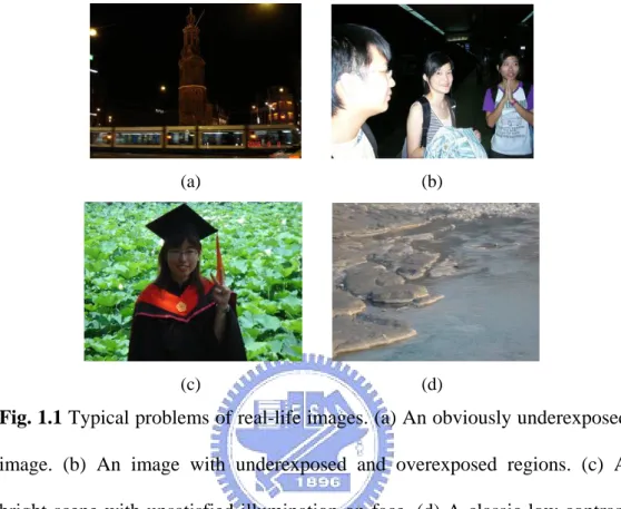
Fig. 1.1 Typical problems of real-life images. (a) An obviously underexposed
image. (b) An image with underexposed and overexposed regions. (c) A bright scene with unsatisfied illumination on face. (d) A classic low-contrast image resulted from moist………2
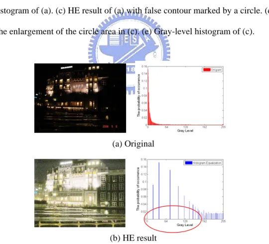
Fig. 1.2 The false contour with HE. (a) Original image. (b) The gray-level
histogram of (a). (c) HE result of (a) with false contour marked by a circle. (d) The enlargement of the circle area in (c). (e) Gray-level histogram of (c)………..………...4
Fig. 1.3 The wash-out appearance and amplified noises with HE. (a) Original
image and its corresponding gray-level histogram. (b) HE result and its corresponding gray-level histogram………...……….4
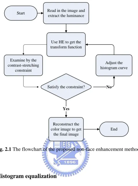
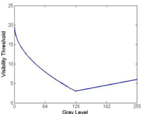
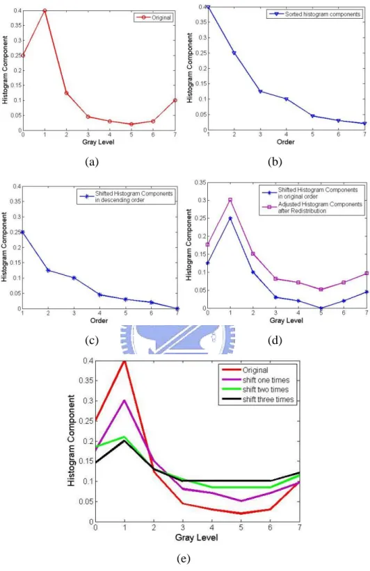
Fig. 2.1 The flowchart of the proposed non-face enhancement method...…..10 Fig. 2.2 Visibility thresholds related to the luminance………...12 Fig. 2.3 An example to illustrate the proposed adjustment method. (a)
Original histogram. (b) The sorted histogram components of (a). (c) The result of shifting (b) one time. (d) The corresponding histograms after shifting one time and redistributing. (e) Several results treated by different shift times……….…………..17
Fig. 2.4 An example to illustrate the procedure of avoiding over-adjustment
……….19
Fig. 2.5 An example to illustrate the proposed method. (a) Original image.
(b)-(e) The enlargement of part of the results treated by 0-3 shift times. (f)-(g) The enlargement of part of the results treated by 4 and 5 shift times. (h) The enlargement of part of the results treated by 4.6 shift times for avoiding over-adjustment. (i) The original and the final adjusted histogram curve………....………21
Fig. 3.1 Some results using different enhancement methods with the images
in the right column being the enlarged parts of the images in the left column. (a) Original image. (b) HE. (c) Capra’s algorithm [8]. (d) Our proposed non-face enhancement method. (e) Picasa software [2]…..23
Fig. 3.2 A result using exposure correction method with the images in the
right column being the enlarged parts of the images in the left column. (a) Original image. (b) Battiao’s algorithm……….24
Fig. 3.3 The flowchart of the proposed face enhancement method……...….25 Fig. 3.4 Statistic of skin locus………...……..26 Fig. 3.5 An example of skin recognition. (a) Original image. (b) Recognized
skin map by the skin locus. (c) Result after Morphological processing………27
Fig. 3.6 A simulated camera response curve………28 Fig. 3.7 An example of the exposure correction method (a) Original image. (b)
Result of the exposure correction method………...…29
Fig. 3.8 An example of measurement of Mdistance with d = 2. (a) A skin map
Mskin. (b) Two connected components in Mskin are split to
and where the symbol ‘-’ means the infinite values. (c)-(d)
Each connected component is dilated respectively until the halting
condition occurs. (e) Combine and with the
smallest values. (f) Substitute the left ‘-’ in M
1 tan ce dis M 2 tan ce dis M 1 tan ce dis M Mdis2 tan ce
distance for the values t+1
to obtain the final Mdistance………....………31
Fig. 3.9 The skin map (a) and its corresponding distance map (b)….………32 Fig. 3.10 The distance map (a) and its corresponding weight map (b) by
power-law function with brighter pixels representing smaller weight value. The bottommost (c) is the final result of our proposed face enhancement method.………..………33
Fig. 4.1 A normal photo enhanced by difference techniques…………...…..37 Fig. 4.2 A photo with shadow areas enhanced by different techniques…....38 Fig. 4.3 An image with a backlight condition enhanced by different method
… … … . 3 9
Fig. 4.4 A dark scene image enhanced by different methods………..40 Fig. 4.5 The original images in the left column and with their corresponding
results treated by our proposed method in the right column...………41
Fig. 4.6 A face image in a dark scene enhanced by different techniques……43 Fig. 4.7 A face image with a backlight condition enhanced by different
methods………44
Fig. 4.8 The original images in the left column and with their corresponding
CHAPTER 1
INTRODUCTION
1.1 Motivation
Due to the rapid development of image capturing device techniques in recent years, digital cameras and camera phones have been widely used in our life. We can find various applications of automatic post-processing or real-time processing for real-life images, such as digital cameras, portable photo printers, Adobe Photoshop [1] and Picasa [2] which is a popular software for people to share photos with on-line album or use on-line photo printing services. However, the limitation of capturing devices and the improper illumination condition may lead to unpleasant image quality. Fig. 1.1 illustrates four common problems in real-life images. Fig. 1.1(a) represents an underexposed problem. Fig. 1.1(b) has both underexposed and overexposed regions simultaneously. Underexposed and/or overexposed problems are easy to take place in a night scene or resulted from using the photoflash. Fig. 1.1(c) shows that the scene possesses a bright background, but the human face is relatively dark resulted from a back-light circumstance. Fig. 1.1(d) shows a low-contrast photo influenced by fog or moist.
Therefore, it is worth mentioning that an automatic and efficient quality improvement in real-life images becomes more and more important. Users neither need to have the knowledge of image processing nor need to learn complicated operation of image processing software. In this thesis, we will present a new approach of image enhancement to solve these four problems
mentioned above. The detail of our proposed method will be described in Chapter 2 and Chapter 3.
(a) (b)
(c) (d)
Fig. 1.1 Typical problems of real-life images. (a) An obviously underexposed
image. (b) An image with underexposed and overexposed regions. (c) A bright scene with unsatisfied illumination on face. (d) A classic low-contrast image resulted from moist.
1.2 Review of Related Works
In general, there are three kinds of methods for image enhancement: (1) histogram-based methods [3-6];
(2) gray-level transform based methods [3, 7-8]; (3) exposure-based methods [9-10].
Conventional histogram equalization (HE) technique [3] is one of histogram-based methods. It is a non-linear mapping which approximately produces discrete equivalence of a uniform probability density function. This
method spreads out values occurring more frequently and compresses values
occurring less frequently to gain a higher contrast. However, HE fails to
produce pleasant pictures owing to three common drawbacks [11]: (1) wash-out appearance;
(2) false contour; (3) amplified noises.
The examples of these drawbacks are given in Fig. 1.2 and Fig. 1.3. In Fig. 1.2 (c), there is an obvious false contour in the sky area. In Fig. 1.3(b), there are not only noises in the background area, but also wash-out appearance in the foreground area.
Several advanced HE techniques [4-6] have been proposed to improve the conventional technique. The global HE method, such as bi-histogram equalization proposed by Kim [4] and dualistic sub-image histogram equalization proposed by Wang et al. [5], separates histogram into two parts according to mean or median, and then the conventional HE is applied on each of the two separated histograms. Based on the limitation on contrast-stretching of global HE, Pizer et al. [6] provided a local HE called adaptive histogram equalization. First, an image is divided into several blocks, and then the HE technique is applied on each block. Finally, the resulted blocks are fused together by bilinear interpolation. The aim of the above-mentioned methods is to obtain the contrast as higher as possible without considering over-contrast problems for real-life images.
(a) (b)
(c) (d) (e)
Fig. 1.2 The false contour with HE. (a) Original image. (b) The gray-level
histogram of (a). (c) HE result of (a) with false contour marked by a circle. (d) The enlargement of the circle area in (c). (e) Gray-level histogram of (c).
(a) Original
(b) HE result
Fig. 1.3 The wash-out appearance and amplified noises with HE. (a) Original
image and its corresponding gray-level histogram. (b) HE result and its corresponding gray-level histogram.
Gray-level transform-based methods (e.g., power-law transforms [3] and logarithm transforms [3], etc.) use a mapping function of the form s = T(r), where T is a transform function that maps a gray level r into a gray level s. These techniques are popular for commercial purposes [3] applied to a variety of devices. However, these transform functions need device-dependent parameters to decide the transform curve. Global gray-level transform methods [3] produce applicable results for either underexposed images or overexposed images by selecting proper parameters in advance. In addition, as both underexposed and overexposed problems exist simultaneously, the global methods are incapable of overcoming both highlight and lowlight regions. Moroney [7] proposed a new approach of image enhancement based on pixel-by-pixel gamma correction with a non-linear masking. Briefly, this gamma correction of each pixel depends on the values of its neighboring pixels. However, it may have halo effects resulted from discontinuous intensity of edges. Afterward, Capra et al. [8] improved this method by combining the low pass filter and edge-preserving filter to reduce the halo effect near contrast sharp boundaries. Although this method can solve the problem that the image has over-exposed and under-exposed regions simultaneously, it may reduce the global contrast.
Exposure-based methods utilize the transformation between light and the luminance of the objects for exposure correction. Battiato et al. [9] proposed a camera response curve for adjusting the exposure level by content dependent. The algorithm identifies the visually relevant regions and calculates the offset between the average brightness of regions of interest and the user-defined satisfied brightness. For the sake of modifying the original illumination to the
satisfied illumination, it utilizes the camera response curve to transform each pixel value based on the offset value. This method is suitable for real-time purpose, such as handset devices. It can produce a satisfied result in interesting regions, but it may lead to worse illumination in other regions. Safonov et al. [10] developed an enhancement algorithm including global and local correction of various exposure defects based on contrast stretching and alpha-blending of brightness of the original image and estimation of reflectance. Although this method is good at local shadow correction, it is a high computational complexity method.
For real-life images, current contrast enhancement technique may either fail to produce satisfactory and undistorted image owing to adjust the contrast excessively, or cannot be improved appropriately both in regions of interest, especially face, and in the background. In this thesis, real-life images with/without face regions are treated by different methods. For non-face images, we propose an effective enhancement method regarding just-noticeable-difference (JND) of human visual system (HVS) as a contrast-stretching constraint to remove the disadvantages of histogram equalization. For face image, we improve our proposed method and combine exposure correction by skin dependent to produce appropriate contrast in background and satisfied illumination in skin regions.
1.3 Organization of the Thesis
This thesis is composed of five chapters. In Chapter 1, previous works are introduced. In Chapter 2 and Chapter 3, we will propose solutions to automatically improve image quality for non-face and face images,
respectively. Several experimental results and comparisons will be shown in Chapter 4. Finally, we will give a conclusion and future work in Chapter 5.
CHAPTER 2
THE PROPOSED NON-FACE ENHANCEMENT
METHOD
The objective of image enhancement is to produce a more suitable result than an original image for a specific purpose. For the application of real-life image enhancement, keeping the sense of reality of the image without artifacts is the most important criterion. For example, if we take a picture at night, we do not hope this photo look like daytime after using image enhancement techniques.
As mentioned previously, HE fails to produce pleasant pictures owing to three drawbacks: (1) wash-out appearance; (2) false contour; (3) amplified noises. Before explaining the proposed method, we will analyze what factors cause these defects. According to the two histograms given in Fig. 1.2, because of the occurrence probability value of histogram bin 255 is abnormally high in the original image, HE causes a serious gap for those pixels with gray values 254 and 255 in the original image. If these two kinds of pixels are neighbors, this will cause false contours. In Fig. 1.3, most pixels have low luminance in the original image. This makes the contrast-stretching by HE very excessive in the low luminance and the medium luminance push toward to the higher grayscales. This will amplify the noises in the dark regions and look like the wash-out appearance in the whole image. In conclusion, when the histogram of an image has the characteristic of high amplitude at few peaks or excessive concentration at small continuous gray
levels, it is difficult to produce a proper result by the HE technique.
Based on the discussion above, we regard JND as a constraint on contrast stretching. If the original histogram curve exceeds a limitation, it is possible that the image is characterized by the problems mentioned above. Therefore, we try to modify the histogram curve to become not only similar to the original histogram curve but also qualify to the restriction. In other words, we use the modified HE mapping to make the contrast as greater as possible without producing artifacts.
In this chapter, a new approach of image enhancement for real-life image is presented. We use the HE technique and regard the JND of HVS model as a contrast-stretching constraint to avoid the artifacts mentioned previously. In Section 2.1, we will introduce the conventional histogram equalization method. In Section 2.2, the contrast-stretching constraint based on JND is provided. In Section 2.3, we present a new approach of adjustment of histogram curve in Section 2.4. In section 2.5, the color construction method is proposed. Fig. 2.1 is the flowchart of our proposed method.
Furthermore, for real-life images, skin regions are the most relevant parts by human perception. We will improve our framework to treat skin problems especially and describe this in Chapter 3.
Start
Use HE to get the transform function
Satisfy the constraint? Read in the image and extract the luminance
Examine by the contrast-stretching constraint Adjust the histogram curve End No Yes Reconstruct the color image to get
the final image
Fig. 2.1 The flowchart of the proposed non-face enhancement method.
2.1 Histogram equalization
Histogram equalization (HE) [3] is a non-linear mapping which approximately produces the discrete equivalence of a uniform probability density function. Before presenting the HE technique, we need to extract the luminance Y at spatial coordinate (x, y) of the original image by
) 1 1 . 2 ( ). , ( 114 . 0 ) , ( 587 . 0 ) , ( 299 . 0 ) , (x y = ⋅R x y + ⋅G x y + ⋅B x y − Y
After obtaining the gray values of the original image, let variable k represent the gray level in the interval [0, 255] of an image. Then, the probability p of the occurrence of gray level k in an image is calculated with
, ) ( N n k p = k (2.1-2)
where N is the total number of pixels in the image, and nk is the number of
pixels of gray value k. Next, we describe the mapping function of the form s = T(k), where T is a transform function that maps a gray level k into a gray level s. The transform function is denoted as follows.
. 255 ) ( 255 ) ( 0 0
∑
∑
= = ⋅ = ⋅ = = k i i k i n n i p k T s (2.1-3)2.2 Contrast-stretching constraint based on JND
Before explaining the constraint, we introduce the concept of JND in advance. In the field of image processing, just-noticeable-difference (JND) is the ability of distinguishing the luminance change with human visual system (HVS). In other words, JND is the smallest difference of the luminance change which is detectable by human eyes. We adopt the JND model proposed by Chou and Li [12]. Fig. 2.2 illustrates the smallest detectable difference of each possible gray level by their experiment. As can be indicated by Fig. 2.2, it is relatively sensitive to the change of medium gray level by human visual system. On the contrary, it is relatively not sensitive to the change of dark or bright background. The perceptual model for evaluating the visibility threshold of JND is denoted by
(
)
1) -(2.2 127 3 127 127 3 127 1 ) ( 5 . 0 0 ⎪ ⎩ ⎪ ⎨ ⎧ > + − ⋅ ≤ + ⎟ ⎟ ⎠ ⎞ ⎜ ⎜ ⎝ ⎛ ⎟ ⎠ ⎞ ⎜ ⎝ ⎛ − ⋅ = k for k k for k T k JND γwhere k is the gray value within [0, 255] and the parameters T0 and γ
depend on the viewing distance between testers and the monitor taken by experiment.
Fig. 2.2 Visibility thresholds related to the luminance.
Real-life image enhancement should not only focus on contrast stretching, but also try to prevent enhancing the areas where the difference of illumination is unnoticeable from producing artifacts. We use this concept to design an examination function which can use to judge if the HE technique is suitably applied to an image. The HE technique uses the information of the occurrence probability of each gray level to determine the amplitude of contrast stretching. Therefore, for any two consecutive gray levels k-1 and k, the mapping function by HE yields corresponding gray levels T(k-1) and T(k). The difference between T(k-1) and T(k) represents the amplitude of contrast stretching. In order to avoid over-contrast-stretching by the HE technique, we give a constraint that for every two consecutive gray levels k-1 and k, which is not distinguishable by human eyes, the difference between T(k-1) and T(k) should not be larger than the JND value of T(k). Based on this constraint, the examination function is denoted as follows:
) 2 2 . 2 ( ) ( 255 ) 1 ( ) ( , 255 0 , )) ( ( ) 1 ( ) ( , − ⋅ = − − ⎩ ⎨ ⎧ − − < ∀ ≤ ≤ k p k T k T otherwise d unqualifie is histogram The k k k T JND k T k T if qualified is histogram The
The examination function can help us to avoid enhancing regions with unnoticeable difference to be perceived. Through the examination function, we can determine whether the HE technique is suitably applied to an image for enhancement.
2.3 Adjustment of histogram curve
As indicated in previous discussion, we can use the examination function to determine if it is suitable to apply the HE technique in an image to do enhancement. If it is suitable, the HE technique can be applied to enhance the image directly without producing artifacts. Otherwise, we must adjust the occurrence probability values to qualify the constraint. If the adjusted histogram curve is smoother, the constraint is more possibly satisfied.
Note that keeping the monotonic property of the histogram of an image is the most important criterion. This means that for any two gray levels h and k, if p(k)>p(h), then p(T(k))>p(T(h)). As a result, our adjustment approach is accomplished by making the histogram curve smoother and preserving the monotonic property. We eliminate the higher probability of occurrence of histogram and then redistribute the eliminated value over all grayscales uniformly. This method can help eliminate the high peaks of histogram or spread out the over-concentration probabilities at small continuous gray levels with lower probabilities. The procedure of the adjustment approach contains three phases: sort, shift, and redistribution. These three phases are described as follows:
) (i
p′
occurrence of gray level i, and represents the adjusted histogram
component. Let n denote the current shift times and initialize to be zero. In order to preserve the monotonic property, we need to sort the distinct histogram components in descending order. Let L denote the number of distinct histogram components and ordern(i) be the ith element sorted histogram components, where i is within the interval [1, L] and n is the
current shift times. Therefore, and represent the
biggest and smallest original probability value respectively without adjustment. Fig. 2.3(a) gives an example of a histogram with 7 histogram components. ) 1 ( 0 order order0(L) . 1 . 0 ) 7 ( , 03 . 0 ) 6 ( , 02 . 0 ) 5 ( , 03 . 0 ) 4 ( , 045 . 0 ) 3 ( , 125 . 0 ) 2 ( , 4 . 0 ) 1 ( , 25 . 0 ) 0 ( = = = = = = = = p p p p p p p p
There are 7 distinct histogram components (L=7) and its ordered set (see Fig. 2.3(b)) is . 02 . 0 ) 7 ( , 03 . 0 ) 6 ( , 045 . 0 ) 5 ( , 1 . 0 ) 4 ( , 125 . 0 ) 3 ( , 25 . 0 ) 2 ( , 4 . 0 ) 1 ( 0 0 0 0 0 0 0 = = = = = = = order order order order order order order
z Shift: After sorting, we shift the histogram components according to the following rules. First, the n-biggest values in sorted histogram components are discarded. That is, if n=2, order (1) and order0 0(2) are
discarded. Next, each sorted component substitute is by the next n sorted component. Then, the shifted and sorted components are transformed into a histogram as follows:
) 1 3 . 2 ( . )) ( ( 0 255 ..., , 1 , 0 ) ( ) ( 1 0 0 − + = ⎩ ⎨ ⎧ > = ≤ = − n k p order v L v if k L v if v order k S
The procedure for shifting the histogram components in Fig. 2.3(b) (n=1) is shown in the following.
. 1 . 0 ) 7 ( 03 . 0 ) 6 ( 02 . 0 ) 5 ( 03 . 0 ) 4 ( 045 . 0 ) 3 ( 125 . 0 ) 2 ( 4 . 0 ) 1 ( 25 . 0 ) 0 ( = = = = = = = = p p p p p p p p histogram Original 02 . 0 ) 7 ( 03 . 0 ) 6 ( 045 . 0 ) 5 ( 1 . 0 ) 4 ( 125 . 0 ) 3 ( 25 . 0 ) 2 ( 4 . 0 ) 1 ( 0 0 0 0 0 0 0 = = = = = = = order order order order order order order components Sorted 02 . 0 ) 7 ( 03 . 0 ) 6 ( 045 . 0 ) 5 ( 1 . 0 ) 4 ( 125 . 0 ) 3 ( 25 . 0 ) 2 ( 4 . 0 ) 1 ( 0 0 0 0 0 0 0 = = = = = = = order order order order order order order components Sorted 0 ) 7 ( 02 . 0 ) 6 ( 03 . 0 ) 5 ( 045 . 0 ) 4 ( 1 . 0 ) 3 ( 125 . 0 ) 2 ( 25 . 0 ) 1 ( 1 1 1 1 1 1 1 1 = = = = = = = = order order order order order order order n Î 045 . 0 ) 7 ( 02 . 0 ) 6 ( 0 ) 5 ( 02 . 0 ) 4 ( 03 . 0 ) 3 ( 1 . 0 ) 2 ( 25 . 0 ) 1 ( 125 . 0 ) 0 ( = = = = = = = = S S S S S S S S histogram d Transforme Zero padding
Figs. 2.3(c) and (d) illustrate the shifted sorted histogram components and the corresponding histogram.
z Redistribution: After obtaining the new shifted histogram components, the difference between original and shifted histogram components are redistributed uniformly over all grayscales. This redistribution function is denoted by
(
)
) 2 3 . 2 ( 1 ,..., 2 , 1 , 0 ) ( ) ( ) ( ) ( 1 1 0 − − = + = ′ ⎟⎟ ⎠ ⎞ ⎜⎜ ⎝ ⎛ − =∑
− = g k dif k S k p i S i p g dif g iwhere g is the number of grayscales. Therefore, the examples of redistributed results are given as follows.
. ) 7 ( 09625 . 0 ) 7 ( ) 6 ( 05325 . 0 ) 6 ( ) 5 ( 05125 . 0 ) 5 ( ) 4 ( 05325 . 0 ) 4 ( ) 3 ( 05425 . 0 ) 3 ( ) 2 ( 15125 . 0 ) 2 ( ) 1 ( 30125 . 0 ) 1 ( ) 0 ( 17625 . 0 ) 0 ( 05125 . 0 8 41 . 0 dif S p dif S p dif S p dif S p dif S p dif S p dif S p dif S p dif + = = ′ + = = ′ + = = ′ + = = ′ + = = ′ + = = ′ + = = ′ + = = ′ = =
Fig. 2.3(e) shows the results treated by different shift times. It can be noted that the more shift times there are, the smoother the curve is. As a result, through increasing the shift times, there should be a smallest shift times such that the adjusted histogram is qualified.
(a) (b)
(c) (d)
(e)
Fig. 2.3 An example to illustrate the proposed adjustment method. (a) Original histogram. (b) The sorted histogram components of (a). (c) The result of shifting (b) one time. (d) The corresponding histograms after shifting one time and redistributing. (e) Several results treated by different shift times.
2.4 Prevention for over-adjustment
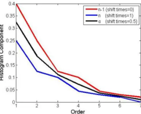
The more number of shift times are, the greater changing of original histogram components is. However, the smoother histogram curve leads to the less amplitude of contrast-stretching. Through the adjustment approach described in previous section, we can get the smallest shifted times n such that the shifted histogram is qualified. In order to avoid over-adjustment, we get an interpolated histogram by
. 255 ,..., 2 , 1 , 0 )) ( ( ) ( ) 1 ( ) ( ) ( ' 1 0 1 = = ⋅ − + ⋅ = − − k k p order v v order v order k p α n α n (2.4-1)
where α∈[0,1] . Then, the differences between original histogram
components and the new histogram components are
redistributed uniformly to get the final histogram components.
) (k p′ ) (k p
(
)
) 2 4 . 2 ( 255 ,..., 2 , 1 , 0 ) ( ) ( ) ( ) ( 256 1 255 0 − = + = ′′ ⎟ ⎠ ⎞ ⎜ ⎝ ⎛ − ′ =∑
= k dif k S k p i p i p dif iWe adopt bisection method to find the smallest α such that the shifted histogram can qualify the constraint. Fig. 2.4 illustrates an example of the procedure. The red curve and blue line show the sorted histogram components treated by n = 0 and n = 1 respectively. The black curve shows the interpolation of the two curves. (α= 0.5)
Fig. 2.4 An example to illustrate the procedure of avoiding over-adjustment.
2.5 Color reconstruction
After previous steps, we can get the modified gray values . Then,
color reconstruction is done by using the following formulation [13] to prevent relevant hue shift and color desaturation. This method is denoted by
Y ′
(
)
(
)
(
)
⎪ ⎪ ⎪ ⎩ ⎪ ⎪ ⎪ ⎨ ⎧ ⎟⎟ ⎠ ⎞ ⎜⎜ ⎝ ⎛ − + + ′ ⋅ = ′ ⎟⎟ ⎠ ⎞ ⎜⎜ ⎝ ⎛ − + + ′ ⋅ = ′ ⎟⎟ ⎠ ⎞ ⎜⎜ ⎝ ⎛ − + + ′ ⋅ = ′ ) , ( ) , ( ) , ( ) , ( ) , ( ) , ( 2 1 ) , ( ) , ( ) , ( ) , ( ) , ( ) , ( ) , ( 2 1 ) , ( ) , ( ) , ( ) , ( ) , ( ) , ( ) , ( 2 1 ) , ( y x Y y x B y x Y y x B y x Y y x Y y x B y x Y y x G y x Y y x G y x Y y x Y y x G y x Y y x R y x Y y x R y x Y y x Y y x R (2.5)where R, G, and B are the input color values.
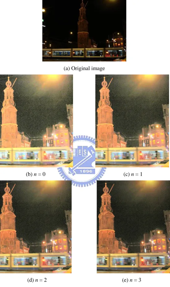
Finally, there is an example to illustrate the whole proposed method in Fig. 2.5. First, there is a dark scene in Fig. 2.5(a). Through the examination function, its corresponding histogram is not qualified, so the adjustment method is applied. Through increasing the shift times, we can find a smallest shift times (n = 4.6) such that the adjusted histogram can be qualified. Figs. 2.5(b) through (h) show the results treated by different shift times. It can be seen that the noises in the background are decreasing and the over-exposed areas are being improved. Fig. 2.5(i) shows the original histogram curve and the adjusted curve applied by our proposed adjustment approach.
(a) Original image
(b) n = 0 (c) n = 1
(d) n = 2 (e) n = 3
Fig. 2.5 An example to illustrate the proposed method. (a) Original image.
(b)-(e) The enlargement of part of the results treated by 0-3 shift times. (continues)
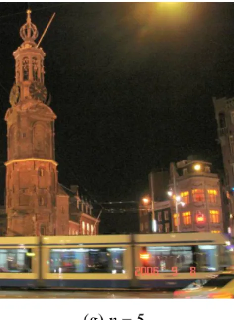
(f) n = 4 (g) n = 5
(h) n = 4, α=0.6 (i)
Fig. 2.5 An example to illustrate the proposed method. (f)-(g) The
enlargement of part of the results treated by 4 and 5 shift times. (h) The enlargement of part of the results treated by 4.6 shift times for avoiding over-adjustment. (i) The original and the final adjusted histogram curve.
CHAPTER 3
THE PROPOSED FACE ENHANCEMENT
METHOD
It is straightforward that skin regions, especially faces, in real-life images are the most visually interesting areas. Most conventional image enhancement techniques [3-8, 10-11] do not give a special treat for the improper lighting condition in skin regions. Hence, these enhancement techniques either improve obviously for the unsuitable illumination in skin regions or fail to offer sufficient contrast in skin regions. If the contrast in skin regions is insufficient, the skin regions may seem to be wash-out appearance and unnatural (see Figs. 3.1(b) through (e)). On the other hand, some techniques [9, 14-15] were provided to enhance face part in an image, for the other part, they can not provide a satisfied result.
Battiato et al. [9] proposed an exposure correction with camera response curve improved by skin dependent techniques. The basis of adjusting illumination in a whole image is based on the difference between the average luminance of skin regions and the ideal pre-defined luminance. This technique can produce a satisfied result in skin regions, but it may fail to produce a suitable result in non-skin regions. Fig. 3.2 shows the satisfied illumination in skin regions, but the background regions are distorted.
(a)
(b)
(c)
(d)
(e)
Fig. 3.1 Some results using different enhancement methods with the images
in the right column being the enlarged parts of the images in the left column. (a) Original image. (b) HE [3]. (c) Capra’s algorithm [8]. (d) Our proposed non-face enhancement method. (e) Picasa software [2].
(a)
(b)
Fig. 3.2 A result using exposure correction method with the images in the
right column being the enlarged parts of the images in the left column. (a) Original image. (b) Battiato’s algorithm.
Since our proposed non-face enhancement method can only treat non-face images well, for those face images, the skin part may not be treated well. In this chapter, we will provide a method to treat both face and non-face regions. The proposed method integrates our non-face enhancement and the exposure correction method proposed by Battiato et al [9]. This exposure correction method uses the mean luminance of skin regions as a reference point. Then, we can apply exposure correction method by skin content to get an image with satisfied skin regions. After obtaining the results of non-face enhancement method defined Ynon-skin, and exposure correction method defined
Yskin, a distance map can help us to fuse these two results. Fig. 3.3 shows the
Fig. 3.3 The flowchart of the proposed face enhancement method.
3.1 Skin recognition by skin locus model
Before applying the exposure correction by skin dependent techniques, we should recognize skin pixels in advance. We would like to determine all possible skin pixels with multiple light source or changing illumination conditions. Therefore, we choose the skin locus model defined in [16]. To reduce the illumination dependence, this technique is based on the
plane by normalized RGB space (
) , (r g ) ( , ) ( R G B g g B G R R r + + = + + = ).
Through the experiment, Fig. 3.4 shows the r-g skin histogram in diverse illumination condition from a 1CCD camera.
Fig. 3.4 Statistic of skin locus
By this statistical information, the skin color cluster in plane
occupies a shell-shape curve. A membership function to the skin locus is a pair of quadratic functions denoting the upper and lower bound of the cluster. Pixels can be labeled as skin pixels using the skin locus constraint denoted as follows: ) , (r g ) 1 . 3 ( ) 33 . 0 ( ) 33 . 0 ( 1766 . 0 5601 . 0 776 . 0 1452 . 0 0743 . 1 3767 . 1 , 0 6 . 0 2 . 0 & 0004 . 0 & ) ( & ) ( , 1 2 2 2 2 − + − = + ⋅ + ⋅ − = + ⋅ + ⋅ − = ⎩ ⎨ ⎧ < > > < < = g r W r r lower r r upper otherwise r W lower g upper g if skin
where skin=1 representing a skin pixel and skin=0 representing a non-skin pixel. The variable W is to avoid labeling whitish pixels as skin. Therefore, we can process an image pixel-by-pixel using this constraint and record the
result in a skin map, , with = 1 representing a skin pixel and
= 0 representing a non-skin pixel(see Fig. 3.5(b)). Then, the skin map should be refined by Morphological operation [3] to eliminate the noises and fill the holes (see Fig. 3.5(c)). In order to speed up the latter procedure described in Section 3.3, we can use the bilinear interpolation of a factor of
skin M Mskin(x,y) ) , (x y Mskin
1/4 to scale the original image at first to obtain a smaller size of Mskin.
(a)
(b) (c)
Fig. 3.5 An example of skin recognition. (a) Original image. (b) Recognized
skin map by the skin locus. (c) Refined skin map after morphological processing.
3.2 Exposure correction method
The exposure correction method is accomplished by a simulated camera response curve [17]. This curve shows an evaluation of light value q, called “light quantity”, transformed to the final pixel values I by the camera sensor (see Fig. 3.6). This camera response curve f can be presented by
C Aq e I q f ) 1 ( 255 ) ( − + = = (3.2-1)
Fig. 3.6 A simulated camera response curve
Therefore, the exposure correction technique [9] utilized the transformation between light quantity and final luminance to simulate controlling how much light the camera will capture. Based on this transformation, the exposure correction method uses the mean luminance of skin regions as a reference point. First, we extract luminance Y with Eq. (2.1-1) in an original image. After labeling skin pixels, we can get the average luminance Yavg of the skin pixels. A simulated camera response curve
f defined in Eq. (3.2-1) can be used to offset the light quantity difference between Yavg and pre-defined ideal luminance Yideal. The offset of light
quantity is denoted by ) ( ) ( 1 1 avg ideal f Y Y f offset= − − − (3.2-2)
The original luminance values can be modified by
))) , ( ( ( ) , ( 1 y x Y f offset f y x Yskin = + − (3.2-3)
Therefore, the Yskin is the result of the exposure correction method. There is
(a) (b)
Fig. 3.7 An example of the exposure correction method (a) Original image. (b)
Result of the exposure correction method.
3.3 Measurement of distance map
In this section, we define a measurement of a distance map Mdistance.
Mdistance means a distance map recording the distance between each pixel and
its nearest skin pixel. The Yskin and Ynon-skin can be fused together using a
distance map. Before presenting the fusion method, we describe the measurement of a distance map at first.
After labeling the skin pixels in the Mskin, there should be several
connected components of skin regions. Therefore, we use the dilation operation [3] iteratively to estimate the Mdistance. It is the reason that if a pixel
is nearer connected components, it will be dilated earlier. Because the distance between a pixel and different connected components is distinct, the smallest distance should be selected. Therefore, each connected component should be dilated individually and recorded the smallest distance for each pixel. A pre-defined threshold t would be given for setting the number of times of performing dilation procedure. When dilation procedure is stop, the pixels which are not dilated yet represent that they are too far from skin
regions. Therefore, they are all assigned to be t+1 which is the farthest distance recorded in Mdistance. This method is described as follows and there
will be an example to illustrate to procedure in Fig. 3.8.
Notation and initialization: Let d denote the current dilation times and
initialize to be zero. Denote Mdisn tance to be the distance map for the nth
connected component where 1≤n≤C and C is the number of
connected components in a skin map. Initialize the
where it is a skin pixel at coordinate belonging
to the n 0 ) , ( tan x y = Mdisn ce (x,y) th
connected component. Other pixels are initialized to be infinite (see Figs. 3.8(a) and (b)).
Step 1: Add one to the variable d. Dilate each connected component in
one time by a disk structuring element and record the current
dilated pixel at to be d. n ce dis M tan ) , ( tan x y Mdisn ce
Step 2: If , go back to step 1. Otherwise, combine all
with the smallest value at the same position to obtain the distance map M
t
d < Mdisn tance
distance. (see Figs. 3.8 (c) throught (e))
Step 3: Replace all infinite values in Mdistance with value t+1. (see Fig.
3.8(f))
It can be noted that Mskin is the scaled image by a factor of 1/4. We must
up-sample the Mdistance to be the same size of an original image for the later
procedure of fusion. Therefore, a bilinear interpolation by a factor of 4 can be used for this purpose. Fig. 3.9 illustrates an example of distance map.
(a) 1 1 0 0 0 0 1 0 1 1 0 0 0 1 1 0 0 0 1 1 0 0 0 0 0 1 1 0 0 0 0 1 0 1 1 0 0 0 1 1 0 0 0 1 1 0 0 0 0 0 0 0 1 1 1 1 0 1 0 0 2 1 1 0 0 -2 1 0 0 -2 1 1 0 0 1 1 1 1 0 1 0 0 2 1 1 0 0 -2 1 0 0 -2 1 1 -1 1 -1 0 0 -1 0 0 -1 0 0 -1 1 -1 1 -1 0 0 -1 0 0 -1 0 0 -1 1 -2 1 1 -2 1 0 0 -2 1 0 0 -2 1 0 0 -2 1 1 -2 1 1 -2 1 0 0 -2 1 0 0 -2 1 0 0 -2 1 1 -0 0 -0 0 -0 0 -0 0 -0 0 -0 0 -1 tan ce dis M 2 tan ce dis M 0 0 -0 -0 0 -0 -0 0 1 -1 0 1 -1 -0 0 1 -1 0 1 -1 -0 0 1 2 -1 0 1 2 -2 1 2 -2 -0 0 1 2 -1 0 1 2 -2 1 2 -2 -0 0 1 1 1 1 0 1 0 0 2 1 1 0 0 3 2 1 0 0 3 3 2 1 1 0 0 1 1 1 1 0 1 0 0 2 1 1 0 0 3 2 1 0 0 3 3 2 1 1 skin M (b) (c) (d) (e) (f)
Fig. 3.8 An example of measurement of Mdistance with d = 2. (a) A skin map
Mskin. (b) Two connected components in Mskin are split to and
where the symbol ‘-’ means the infinite values. (c)-(d) Each connected component is dilated respectively until the halting condition occurs.
(e) Combine and with the smallest values. (f) Substitute
the left ‘-’ in M 1 tan ce dis M 2 tance dis M 1 tance dis M Mdis2 tance
(a) (b)
Fig. 3.9 The skin map (a) and its corresponding distance map (b) with
brighter pixels representing smaller distance values.
3.4 Fusion
After obtaining Mdistance, Yskin and Ynon-skin, each pixel of the finial
luminance Yfinal(x,y) is a composition of the Yskin and Ynon-skin with Mdistance.
Therefore, there should be a weight map based on Mdistance on the
interpolation process. It is straightforward that if the distance of a pixel is very small, this pixel value should be closer to Yskin. We use the power-law
curve with 0.4 by mapping the narrow range of smaller distance values into a wider range of bigger weight values. This curve can make the composition in the boundary regions between skin and non-skin sharper without halo effects. The combination equation with power-law function is expressed by
( )
(
)
) 4 . 3 ( 1 ) , ( ) , ( ) , ( ) , ( ) , ( , 1 ) , ( 4 . 0 tan ⎟ ⎠ ⎞ ⎜ ⎝ ⎛ + = ⋅ + ⋅ − = − t y x M y x weight y x Y y x weight y x Y y x weight y x Y ce dis skin non skin finalwhere t is the threshold of dilation times defined in Section 3.3. Finally, we
use the same method in Eq. (2.5) with and original luminance Y to
reconstruct the color image. Fig. 3.10 illustrates an example of a weight map and a final result.
final
(a) (b)
(c)
Fig. 3.10 The distance map (a) and its corresponding weight map (b) by
power-law function with brighter pixels representing smaller weight value. The bottommost image (c) is the final result of our proposed face enhancement method.
.
CHAPTER 4
EXPERIMENTAL RESULTS
In this chapter, the experimental results implemented by our proposed non-face enhancement method and face enhancement method are given. In our database, there are about 150 photos including landscapes and portraitists with image resolution about 1280 × 960. These photos include: (1) overexposed and/or underexposed problems; (2) low-contrast problems; (3) normal images with good exposure light. We will give some experimental results and five comparisons with following techniques:
HE technique [3]; Picasa software [2];
Exposure correction (Battiato’s algorithm [9]); Local gamma correction (Capra’s algorithm [8]); Shadow correction (Safonov’s algorithm [10]).
These experimental results and comparisons are shown in Section 4.1 for non-face images and in Section 4.2 for face images.
4.1 Experimental results of non-face images
There are four experiment results and comparisons of non-face images shown in Fig 4.1 through Fig. 4.4. These four results include a normal image, a photo with shadow areas, an image with a backlight condition, a dark scene image. Finally, there are more experimental results shown in Fig. 4.5.
the results treated by different techniques. Through the proposed examination function, the HE technique is suitably applied to this image directly without artifacts. The result of the HE technique is shown in Fig. 4.1(b) which is the same as the result of our proposed method in Fig. 4.1(g). Figs. 4.1(c) through (f) show the comparisons with Picasa, Battiato’s algorithm, Capra’s algorithm and Safonov’s algorithm. Fig. 4.1(d) shows a slight over-exposed look in the regions of lotus leaves. In Fig. 4.1(e), there is a suitable result in local regions but the global contrast is decreasing. The results in Figs. 4.1(c) and (f) are almost the same as the original image. By comparing all results, we can see that the result of our proposed method is more vivid and high contrast.
Second, there is an image with shadow areas given in Fig. 4.2(a), and others are the results treated by different techniques. Through the proposed examination function, the HE technique is suitably applied to this image directly. Therefore, we can see that the results in Fig. 4.2(b) applied by the HE technique and (g) applied by our method are the same. By comparing other results in Figs 4.2(c) through (f), we see that the result of our proposed method is both good at shadow areas and other areas.
Third, Fig. 4.3(a) illustrates an image with over-exposed and under-exposed regions simultaneously. Through the examination function, the HE technique is not suitably applied to this image. We can see that in Fig 4.3(b), although the dark area is enhanced clearly by applying the HE technique, there is an obvious false contour in the sky area. In Fig. 4.3(d) applied by Battiato’s algorithm, although the dark area is enhanced clearly, the details in the sky area are loss. The result of Picasa in Fig 4.3(c) is almost the same with the original image. Figs 4.3(e) and (f) applied by Capra’s
method and Safonov’s method have slight improvement in shadow areas, and the global contrast of the results are reducing. In Fig 4.3 (g), our result not only has obvious improvement in shadow areas, but also keeps the details in the sky area.
Fourth, there is a dark scene in Fig. 4.4(a). The result in Fig. 4.4(b) applied by the HE technique shows that background noises have been amplified and there is a halo-effect in the light area. In Fig. 4.4(d) applied by Battiato’s method, there is also an obvious halo-effect in the light area. In Figs. 4.4(c) and (f) treated by Picasa and Safonov’s method, it can be seen that there are few differences between the original images and these two images. The results of Capra’s method and our proposed method in Figs. 4.4(e) and (g) have obvious improvement in detail of the dark area without artifacts. Nothing that Capra’s method is based on pixel-by-pixel gamma correction with a non-linear masking, so it is a high complexity algorithm. By comparing the complexity, our proposed algorithm is accomplished by a modified global HE technique, so our proposed method can execute efficiently and automatically.
As illustrations of the experimental results, it should be pointed out that our proposed examination function can detect effectively if the HE technique is suitably applied to an image. If it is not qualified, our adjustment approach can produce well results without artifacts. Furthermore, there are more experimental results by our proposed method shown in Fig. 4.5.
(a) Original image (b) HE
(c) Picasa software (d) Battiato’s algorithm
(e) Capra’s algorithm (f) Safonov’ algorithm
(g) Our method
(a) Original image (b) HE
(c) Picasa software (d) Battiato’s algorithm
(e) Capra’s algorithm (f) Safonov’ algorithm
(g) Our method
(a) Original image (b) HE
(c) Picasa software (d) Battiato’s algorithm
(e) Capra’s algorithm (f) Safonov’ algorithm
(g) Our method
(a) Original image (b) HE
(c) Picasa software (d) Battiato’s algorithm
(e) Capra’s algorithm (f) Safonov’ algorithm
(g) Our method
Fig. 4.5 The original images in the left column and with their corresponding
4.2 Experimental results of face images
In this section, we will show the experimental results and comparisons of two kinds of face images including a dark scene and a backlight condition shown in Fig. 4.6 and Fig. 4.7 respectively. Finally, there are more experimental results shown in Fig. 4.8.
First, Fig. 4.6(a) illustrates the face photo taken in the dark scene. The result of HE in Fig. 4.6(b) shows the noises are amplified and the face regions are over-exposed. The results applied by Picasa and Battiato’s method in Figs. 4.6(c) and (d) have improvement in skin regions, but the background is still unclear. The result applied by Capra’s method in Fig. 4.6(e) has more distinguishable details in the background, but the face regions seem unnatural influenced by insufficient contrast. Fig. 4.6(f) shows the slight improvement in both background and skin regions by Safonov’s method. By comparing all results, the result of our proposed method in Fig. 4.6(g) shows that there is not only a clearer background, but also satisfied illumination in skin regions.
Second, Fig. 4.7(a) illustrates a face photo taken in a backlight condition. In Fig. 4.6(b), HE still produces a wash-out appearance in skin regions. The results of Figs. 4.6(c), (e) and (f) treated by Picasa, Capra’s method and Safonov’s method still have unsatisfied illumination in face regions. In Figs. 4.6(b), the face regions are both seems unnatural influenced by insufficient contrast in skin regions. Fig. 4.6(d) has satisfied illumination in face regions, but the details in the background are loss. The result of our method in Fig. 4.6(g) has not only appropriate illumination in face regions, but also a suitable background.
(a) Original image (b) HE
(c) Picasa software (d) Battiato’s algorithm
(e) Capra’s algorithm (f) Safonov’s algorithm
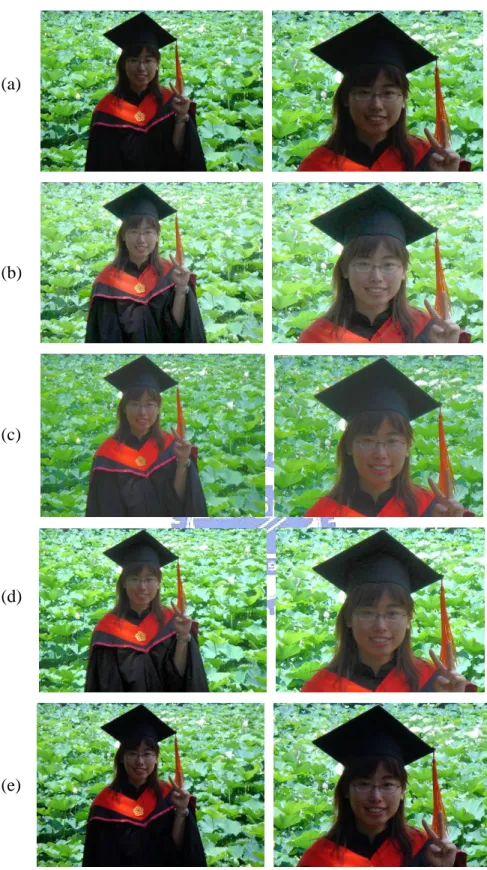
(g) Our method
(a) Original image (b) HE
(c) Picasa software (d) Battiato’s algorithm
(e) Capra’s algorithm (f) Safonov’s algorithm
(g) Our method
Fig. 4.7 A face image with a backlight condition enhanced by different
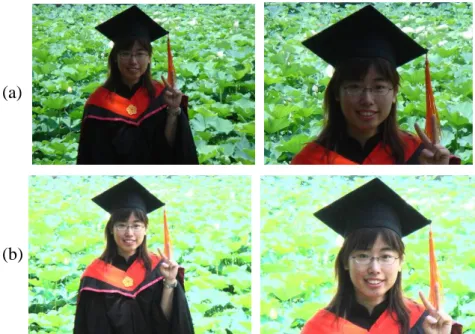
Fig.4.8 The original images in the left column and with their corresponding
CHAPTER 5
CONSLUSION AND FUTURE WORK
In this thesis, we have proposed an automatic and efficient non-face enhancement method and face enhancement method respectively. In the non-face enhancement method, we propose a contrast-stretching constraint based on JND to judge if the HE technique is suitably applied to an image. If it is not qualified, we present an adjustment approach to modify the histogram curve without destroying the monotonic property. In the face enhancement method, we improve our framework by combing our proposed non-face enhancement method and exposure correction technique provided by Battiato et al. [9] to obtain satisfied contrast in the background and appropriate illumination in skin regions. On this combining process, a distance map estimated by iterative morphological operations is used for this fusion purpose. Experimental results show that our proposed method can produce suitable results without artifacts.
It can be noted that our proposed image enhancement method is based on the information of illumination, not colors. Therefore, it may be an interesting approach to extend our concept by combing color HE techniques [18] and the JND model.
REFERENCES
[1] Adobe Photoshop: http://www.adobe.com/products/photoshop/family/, Adobe Systems Inc.
[2] Picasa: http://picasa.google.com/, Google, Inc.
[3] R. C. Gonzalez, and R. E. Woods, Digital Image Processing, 2nd Ed., New Jersey: Prentice-Hall, 2002, ISBN: 0-201-18075-8.
[4] Y. T. Kim, “Enhancement using brightness preserving bi-histogram equalization,” IEEE Transactions on Consumer Electronics, vol. 43, no. 1, pp. 1–8, Feb. 1997.
[5] Y. Wang, Q. Chen, and B.-M. Zhang, “Image enhancement based on equal area dualistic sub-image histogram equalization method,” IEEE Transactions on Consumer Electronics, vol. 45, no. 1, pp. 68–75, Feb. 1999.
[6] S. M. Pizer, E. P. Amburn, J. D. Austin, R. Cromartie, A. Geselowitz, T. Greer, B. H. Romeny, J. B. Zimmerman, and K. Zuiderveld, “Adaptive histogram equalization and its variations,” Computer Vision, Graphics, and Image Processing, vol. 39, no. 3, pp. 355–368, Sep. 1987.
[7] N. Moroney, “Local colour correction using non-linear masking,” IS&T/SID Eighth Color Imaging Conference, pp. 108-111, 2000.
[8] A. Capra, A. Castrorina, S. Corchs, F. Gasparini, and R. Schettini, “Dynamic range optimization by local contrast correction and histogram image analysis,” IEEE International Conference on Consumer Electronics (ICCE’06), pp. 309-310, Jan. 2006.
[9] S. Battiato, A. Bosco, A. Castorina, and G. Messina, “Automatic image enhancement by content dependent exposure correction,” EURASIP
Journal on Applied Signal Processing, vol. 2004, no. 12, pp. 1849-1860, 2004.
[10] I.V. Safonov, M. N. Rychagov, K. Kang, S. H. Kim, “Automatic correction of exposure problems in photo printer,” IEEE Tenth International Symposium on Consumer Electronics (ISCE '06), pp. 1-6, 2006.
[11] Z.Y. Chen, B. R. Abidi, D. L. Page, and M. A. Abidi, “A generalized and automatic image contrast enhancement using gray level grouping,” IEEE International Conference on Acoustics, Speech and Signal Processing (ICASSP ‘06 Proceedings), vol 2, pp. 965-968, 2006.
[12] C. H. Chou and Y. C. Li, “A perceptually tuned subband image coder based on the measure of just-noticeable-distortion profile,” IEEE Transactions on Circuits and Systems for Video Technology, vol. 5, no. 6, pp. 467-476, Dec. 1995.
[13] S. Sakaue, M. Nakayama, A. Tamura, and S. Maruno, “Adaptive gamma processing of the video cameras for the expansion of the dynamic range,” IEEE Transactions on Consumer Electronics, vol. 41, no. 3, pp. 555-562,1995.
[14] F. Naccari, S. Battiato, A. Bruna, A. Capra, and A. Castorina,” Natural scenes classification for color enhancement,” IEEE Transactions on Consumer Electronics, vol. 51, no. 1, pp.234-239, Feb. 2005.
[15] C. Shi, K. Yu, J. Li, and S. Li,” Automatic image quality improvement for videoconferencing,” IEEE International Conference on Acoustics, Speech, and Signal Processing, 2004. Proceedings. (ICASSP '04), vol. 3, pp. 701-704.
[16] M. Soriano, B. Martinkauppi, S. Huovinen, and M. Laaksonen, “Skin color modeling under varying illumination conditions using the skin locus for selecting training pixels,” in Proc. Workshop on Real-time Image Sequence Analysis (RISA’00), pp. 43–49, Oulu, Finland, August-September 2000.
[17] S. Battiato, A. Castorina, and M. Mancuso, “High dynamic range imaging for digital still camera: an overview,” Journal of Electronic Imaging, vol. 12, no. 3, pp. 459–469, 2003.
[18] E. Pichon, M. Niethammer, and G. Sapiro, “Color histogram equalization through mesh deformation,” in Proc. International Conference Image Processing, vol. 2, pp. II-117–II-120, Sep. 2003.