行政院國家科學委員會專題研究計畫 成果報告
以模擬進行排序佳化的方法研究及其於生產排程之應用
(3/3)
計畫類別: 個別型計畫
計畫編號: NSC93-2212-E-002-082-
執行期間: 93 年 08 月 01 日至 94 年 07 月 31 日
執行單位: 國立臺灣大學電機工程學系暨研究所
計畫主持人: 張時中
計畫參與人員: 林偉誠、謝旻旻、何元祥、陳嘉偉、朱紹儀、陳俊宏教授
報告類型: 完整報告
處理方式: 本計畫可公開查詢
中 華 民 國 94 年 10 月 12 日
以模擬進行排序佳化的方法研究及其於生產排程之應用(3/3)
Simulation-based Ordinal Optimization Methods with Applications to
Production Scheduling (3/3)
計 畫 編 號:NSC 93-2212-E-002-082
主 持 人:張時中教授
計畫參與人員:林偉誠、謝旻旻、何元祥、陳嘉偉、朱紹儀
陳俊宏教授
執行期限:93 年8 月1 日至94 年7 月31 日
執行單位:國立台灣大學電機工程學系
一、 中文摘要 本報告總結第三年在本計畫的支持下的研究成 果,包括三個層次的排程佳化方法:(1)以平穩 (Stationary)馬可夫決策問題為載具,設計出一個 結 合 模 擬 排 序 佳 化 (Simulation-based Ordinal Optimization) 與 目 標 函 數 值 疊 代 (Simulation-Based Value Iteration, SBVI)的演算法,作為以快 速模擬排序佳化來選擇動態排程法則的理論基 礎。(2)針對反向拍賣競標(reverse auction)市場 機制,建立設計公司的訂單分配與合約製造商的 生產排程決策模型,以計量與模擬分析來探討合 約製造商間在競合關係下的生產排程策略。(3) 以 衛星 取 像 排程 問 題進 行 拉 氏釋 限 (Lagrange relaxation)法與禁忌搜尋法於單機排程應用效能 的分析比較。 關鍵詞:排序佳化、模擬、目標函數值疊代、演 算法設計、反向拍賣競標、生產排程 AbstractThe third year of research efforts developed scheduling methods in three aspects. (1) The design of ordinal optimization-based value iteration algorithm (OOBVI) combines ordinal optimization (OO) with simulation-based value iteration (SBVI) into an efficient method for solving complex stationary Markov decision problems (StMDPs). The method lays a foundation for dynamic composition of production scheduling policies via quick simulation. (2) A reverse auction-based model captures the gaming interactions between order assignments from a
design house and the production
planning/scheduling of individual contract manufacturers (fabs). The model enables quantitative analysis and simulation study of the production planning/scheduling policies in a co-opetition setting. (3) A study compares
Lagrange relaxation-based and Tabu search-based single machine scheduling algorithm over a satellite imaging problem.
Keywords: Ordinal Optimization, Simulation, Value Iteration, Algorithm Design, Reverse Auction, Production Scheduling
二、 緣由與目的
At fab operation control level, major scheduling problems include how wafers should be released into a fab and how they should be dispatched among tools for processing. A popular practitioners’ approach for composing a dispatching policy for the whole fab is to select from the empirical scheduling rules available for individual tool groups. Dispatching rules for each tool group should be designed based on the specific characteristics and operation goals of the tool group. Empirical or heuristic rules are collected for individual tool groups. The industry of VLSI wafer fabrication has indicated a strong need for an efficient simulation tool for dispatching policy composition from the existing library.
Policy composition by using the traditional simulation approaches is not fast enough in computation for fab dispatching. Recent research [1] has shown that comparing relative orders of performance measures converges much faster than the performance measures do. This is the basic idea of ordinal optimization (OO). OO can be used as a means for solving dispatching rule selection problems if our goal is to find a good enough scheduling policy rather than to find an accurate estimate of the performance value of a scheduling rule.
Hsieh et al. [2, 3] has applied OO in conjunction with a technique called optimal
computing budget allocation(OCBA) to dynamic
selection of scheduling rules for fabs and has shown its potential for real applications. However, a homogeneous set of dispatching rules among tool groups is assumed in [2]. As the number of candidate policies grows in a combinatorial way with the number of tool groups, a brute-force application of the OO and OCBA method to selecting a good policy is still infeasible.
In the first year research we designed a fast simulation methodology by an innovative combination of the notions of ordinal optimization (OO) and design of experiments (DOE) to efficiently select a good scheduling policy for fab operation, where the DOE method is exploited to largely reduce the number of scheduling policy combinations among various tool groups to be evaluated by the OO-based simulation. Simulation results of applications to scheduling wafer fabrications show that most of the OO-based DOE simulations require 2 to 3 orders of magnitude less computation time than those of a traditional approach.
The second year of research developed a fast simulation for solving the Markov decision process formulation of dispatching problem by combining ordinal optimization and policy iteration. We also investigated the applicability of re-enforcement learning to Markov decision process formulation of dispatching problems and assessed the needs for a logistic information service provider for the electronics industry of Taiwan.
In the third year of research, we aimed at the following three objectives based on our research results of the first two years:
(1) to design an efficient and simulation-based method for dynamic selection of a production scheduling policy from available options over time,
(2) to model the gaming interactions between order assignments from a design house and the production planning/scheduling of individual contract manufacturers (fabs), and
(3) to further analyze single machine scheduling methods as a decision module in our simulation. 三、 研究進度與成果
III.1 Ordinal Optimization-Based Value Iteration (OOBPI)
In many stationary Markov Decision Problems (StMDPs) modeling of real problems: for instance,
inventory control problems, computer, and communication networks, both the transition probability and cost function must be generated via computer simulation because of problem complexity and uncertainty. Simulation-Based Policy Iteration (SBPI) is a typical solution in these problems. SBPI includes a sequence of policy evaluation and policy improvement steps (Figure 1.1). In Policy evaluation step, we evaluate cost-to-go (CTG) value for each state via simulation of multiple stages. It is the most time-consuming step in SBPI algorithm. It means that if we want to decrease CPU time with a good optimal policy accuracy (PA), we have to shorten the CPU time in the policy evaluation step. Observation of simulation experiments with SBPI indicates that rough estimation accuracy of CTG may lead to good enough policy but much less simulation time. Though the value estimation is rough, policy accuracy improves gradually with iteration process. This motivates our search and idea of improvement approach of algorithm.
In this task, we first propose Simulation-Based Value Iteration (SBVI) ([4]) to solve StMDPs (Figure 1.2). In the policy evaluation step as compared with SBPI, SBVI evaluates stage-wise cost only and adds it to the estimation of CTG from the previous iteration to update the values in current iteration. Estimation of CTG is rougher than that of SBPI in early iterations but still leads to good enough policy and spends less simulation time (Table 1.1). And PA will approach optimal policy with iterations. In the numerical study that compares SBPI with SBVI by a medium dimension problem, simulation time can be saved around two orders in SBVI (Table 1.1) (Figure 1.3) (Figure 1.4) than SBPI(Table 1.2) (Figure 1.5) (Figure 1.6) to get the same level policy accuracy. However, simulation time of SBVI in high PA rapidly grows with PA and problem dimensions.
We further exploit the property that optimal ranking of decisions for each state may have been formed even when CTG estimation accuracy is rough and propose an Ordinal Optimization-Based Value Iteration (OOBVI) algorithm (Figure 1.7) by combining the concept of OO with SBVI. OOBVI adopts the approximate probability of correct selection (APCS) instead of CTG estimation accuracy as the stopping criterion of policy evaluation.
Simulation study of a medium dimension problem shows that OOBVI can save four times of simulation time as compared with SBVI to reach the same PA(Table 1.3) (Figure 1.8) (Figure1. 9).
Further simulation studies show that the growth of simulation time in OOBVI is approximately linear with respect to the increase in PA, which is exponential in SBVI. We therefore project that OOBVI is more efficient than SBVI in large dimension problems.
In the OOBVI described above, the same decision ranking accuracy is used for all states in the policy evaluation step, which is unnecessary. We then propose an innovative idea of variable decision ranking accuracy among states and design a scheme of computing budget allocation over states (CBA-S). The combination of CBA-S with OOBVI may achieve a high PA at a relatively low simulation time. Simulation study of a medium dimension problem shows that OOBVI with CBA-S can save ten folds of simulation time as compared to using OOBVI only.
III.2 Reverse Auction-Based Job Assignment to Foundry Fabs
In most of the production scheduling literature, scheduling methods are developed under the assumption of centrally available information, or distributed information with cooperative behavior. Nevertheless, in a real world supply chain, each entity has its own individual objective and privately held information. The centralized production scheduling does not apply to such problems [5,6].
In this task, we consider a contract manufacturing environment, where there is a job provider who offers a set of jobs and calls for bids from a few fabs to process the jobs. This task assumes a simplified problem, where each job has only one operation and requires a certain processing time of a unit capacity from a foundry service provider. The job processing is non-preemptive; that is, once a job is started, no interruptions are allowed until completion. A job can only be assigned to one fab at a time. Each job has a time window for processing between its release date and due date. If a job is started before the release date or delivered after the due date, there will be a penalty incurred on the foundry service provider. We assume that jobs under consideration are already available for processing.
The job provider out-sources the job processing to qualified fabs and sets for the processing of each job a maximum payment. The fabs are competitive to each other. Each fab has its own private information such as the actual
capacity, the job processing cost, the valuation of getting a job and its objective function. Without knowing such private information of fabs, the job provider cannot do centralized job scheduling. Auction-based job scheduling mechanisms are therefore frequently adopted.
Among various auction markets [7], we consider a reverse auction-based mechanism (Figure 2.1). The objective of the job provider (auctioneer) is to minimize its payment cost of completing all the jobs in hand plus the penalty cost of unassigned jobs (Figure 2.2), if any. By distributing job information to all the qualified fabs (bidders), the job provider solicits individual fabs to bid on the jobs, where a bid on a job specifies the beginning time, the ending time and the discount from the maximum payment for processing the job. In each round of bidding, the job provider first selects the fab that offers the highest discount of each job as the temporary assignment of the job. The initial discounts are zero for all jobs.
Given the temporary discounts on assignments of jobs, a fab then evaluates and schedules to determine whether to offer new bids on various jobs. The new discount offer for a job must be higher than its current value. The objective of a fab is to maximize the payment it may receive from processing the jobs minus the earliness/tardiness penalty for each job not processed within the desired time window of the job(Figure 2.3). Note that the earliness/tardiness penalty of a job is fully compensated by the job winning fab. After the job provider collects the bids from all the fabs, one round of bidding ends. Such a bidding procedure repeats round by round till no new bids from any fabs. The scheduling problem of the bidder is a NP hard scheduling problem itself. We apply the Lagrangian Relaxation to decompose the problem. Because there are several independent decision makers in the auction, the concept of an optimal solution is not suitable to use. We then use the concept of an equilibrium solution to evaluate the result. We define our equilibrium solution as that no entity can benefit from changing its strategy given the other entities’ strategies.
Numerical studies are performed to examine theoptimality ofabidder’sschedule. Thereare two test case designs: medium and overload loading intensity. The optimality metric is the duality gap, which is defined as the cost of dual solution minus the cost of the final and feasible solution divided by the cost of the final and
feasible solution.
A1) Medium case
The loading intensity is 46.66% of the capacity in this case. How the duality gap varies as the LR iteration is shown in (Figure2.4). Since the duality gap goes to zero, an optimal solution is achieved in this case.
A2) Overload case
Its loading intensity is 113.33% of the capacity in this case. The scheduling is expected to be difficult and the dual solution will have many capacity constraint violations. (Figure2.5) shows how the duality gap evolves with respect to the LR iteration. The final duality gap in this case is 1.89%. These preliminary results indicate that the LR solution method leads to near-optimum solutions.
Auction Experiment
This experiment evaluates how the dimension factors such as the number of bidders and the number of jobs may affect the number of auction rounds and the solution. We conjecture that the lager the number of bidders (jobs), the more rounds needed to complete the auction. Our reasoning is that when the number of bidders (jobs) increases, the possibility of counter biddings (the number of bid options) increases and leads to the increase of auction rounds.
B1) Number of bidders
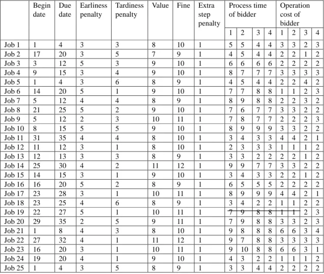
In this case, we change the number of bidders but fix the number of jobs. We compare a 2-bidder and a 4-bidder examples, both with 25 jobs. The 2 bidders of the 2-bidder example have the same parameters as bidder 3 and 4 in the 4-bidder example. In the 4-bidder auction, it takes 12 rounds to complete the auction while it takes 6 rounds in the 2-bidder auction. Results of (Table 2.5 ) match our conjecture.
B2) Number of jobs
In this case, we consider 13 and 25 jobs for the same 4 bidders. The 13 jobs is a subset of the 25 jobs. The bidder and job data is the same as that of B1. In the 25-job auction, it takes 12 rounds to complete the auction while it takes 7 rounds in the 13-job auction. Results of B2 also match our conjecture.
III.3 Comparison of Lagrange Relaxation and Tabu Search-based Single Machine Scheduling
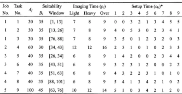
The earth observation satellite, FORMOSAT-2 [1], is designed to periodically monitor and
provide timely imaging data of Taiwan island. The daily imaging scheduling problem of FORMOSAT-2 includes considerations of various imaging requests (jobs) with different reward opportunities, changeover efforts between two consecutive imaging operations (tasks), cloud coverage effects, and the availability of satellite resource. It belongs to a class of single-machine scheduling problems with salient features of job-assembly characteristic, sequence-dependent setup effect, and the constraint of operating time window. The scheduling problem is first formulated as a monolithic integer programming problem, which is NP-hard in computational complexity [2]. An approximation of the weighted penalty of incomplete jobs by penalties of individual tasks facilitates a separable integer programming problem. For problems of such high complexity, dynamic programming and exhaustive search techniques are either too time-consuming or impractical for optimal solutions. Rule-based or heuristic approaches can reduce the computation time drastically but the resultant optimality may be unsatisfactory.
Mathematical programming approaches, such as Lagrangian relaxation [3], have the advantage of computational efficiency when the optimization problems are decomposable. In many cases, the computation time increases almost linearly with the problem size. However, a heuristic is usually needed to modify the dual solution into a feasible solution. In view of the separable problem structure, Lin et al [8] adopted the Lagrangian relaxation and sub-gradient optimization technique to solve the daily imaging scheduling problem of FORMOSAT-2. Based on the dual solution, a greedy heuristic is developed with the help of Lagrangian multipliers to re-allocate imaging tasks to a feasible schedule. This greedy heuristic is quick and easy to implement. However, it could probably be trapped in a local optimum. Intelligent search techniques such as Tabu search can help escape from the local optimal trap.
Tabu search [9] is a meta-heuristic designed for tackling hard combinatorial optimization problems. Contrary to random search approaches such as simulated annealing where randomness is extensively used, Tabu search is based on intelligent searching to embrace more systematic guidance of adaptive memory and learning. Vasquez and Hao [7] introduced a “logic constrained” knapsack formulation for a real world application, the photograph daily imaging scheduling problem of the satellite
SPOT-5 [8], and developed a highly effective Tabu search algorithm. Motivated by their researching findings, Lin and Liao [9] developed a modified Tabu search algorithm which integrated some important ideas including a greedy-based searching process, boundary extension by constraint relaxation, a dynamic Tabu tenure mechanism, intensification, and diversification to make the searching effective and efficient on solving the daily imaging scheduling problem of FORMOSAT-2 (Figure3.1)(Table3.1).
Hybrid methods are promising tools in mixed-integer programming (MIP), as they combine the best features of different methods in a complementary fashion. Examples of linear mixed-integer programming problems include manufacturing scheduling, transportation, cargo-loading, and network routing problem. Long computation time is usually needed to solve these real-life complex scheduling problems.
In [9], Comparative results of 19 classes of 190 realistic daily imaging scheduling problems of FORMOSAT-2 indicated that with the help of exploration over diverse schedules, the Tabu search algorithm was superior in optimality; on the other hand, the Lagrangian relaxation algorithm achieved near dual optimal and had an advantage in computational efficiency (Table3.2). Motivated by above observations, in this paper, two hybrid schemes, CASCADE(Figure3.2) and COMBINATION (Figure3.3), are further developed to generate sound satellite imaging schedules within allowable computation time. CASCADE adopts Tabu search techniques to improve the solution quality of Lagrangian relaxation algorithm directly. COMBINATION then deals with the development of Tabu search-based feasibility adjustment heuristic in Lagrangian relaxation algorithm. These hybrid schemes are expected to exhibit the advantage of providing not only good feasible solutions but also a strong indication on the performance improvement to optimal solution (Table3.3) (Table3.4).
四、 參考文獻
[1] C.-H. Chen, "A lower bound for the correct subset selection probability and its application to discrete-event system simulations," IEEE Transactions
on Automatic Control, vol. 41, no. 8, pp. 1227-1231,
Aug. 1996.
[2] B.W. Hsieh, C.-H. Chen, and S.-C. Chang, "Scheduling semiconductor wafer fabrication by using ordinal optimization-based simulation," IEEE Transactions on Robotics and Automation, vol. 17, no.
5, pp. 599-608, Oct. 2001.
[3] B.-W. Hsieh, S.-C. Chang, C.-H. Chen, “Efficient Selection of Scheduling Rule Combination by
Combining Design of Experiment and Ordinal
Optimization-based Simulation,” Proceedings of ICRA2003, Taipei, Sept., 2003.
[4]M.L.Puterman,“Markov Decision Process,” John Willy & Sons, Inc., NY, 1994.
[5]M. Jin and S.D. Wu,"Coordinating Supplier Competition via Auctions," http://www.lehigh. edu/ ~sdw1/jin1.pdf, August 2004.
[6] M. Fan, J. Stallaert, and A. B. Whinston, “Decentralized Mechanism Design for Supply Chain Organizations Using an Auction Market”, Information
Systems Research, Vol. 14, No. 1, p.1-22, March 2003.
[7] R. Engelbrecht-Wiggans, “Auctions and Bidding
Models: A Survey”, Management Science,
26(2):119-142, 1980.
[8] W.-C. Lin, D.-Y. Liao, C.-Y. Liu, and Y.-Y. Lee, “Daily Imaging Scheduling of An Earth Observation Satellite,”IEEE Transactions on Systems, Man, and
Cybernetics—Part A: Systems and Humans, Vol. 35,
No. 2, pp. 213-223, March 2005.
[9] F. Glover and M. Laguna, Tabu Search, Kluwer Academic Publishers, 1997.
五、 發表論文
1. S.-C. Chang, C.-H. Chen, M.-C. Chang, Y.-H. Ho, “Design of Ordinal Optimization Based-Policy Iteration,” to be submitted to
ICASE2006.
2. S.-C. Chang, M.-M. Hsieh, “Reverse Auction-based Job Assignment among Foundry Fabs,”Proceedings of the 3rd International Conference on Modeling and Analysis of Semiconductor manufacturing, Singapore, Oct.
6-7, 2005, pp. 347-354.
3. W.-C. Lin, S.-C. Chang, "Hybrid Scheduling dor satellite Imaging,” semiconductor wafer fabrication by using ordinal optimization-based simulation," Proceedings of International Conference on Systems, Man and Cybernetics,
Oct. 4-6, 2005, Hawaii.
4.Y.-H. Ho, “Design of Ordinal
Optimization-Based Value Iteration with Computing Budget Allocation” MS Thesis, Dept. of Electrical Engineering, National Taiwan University, Taipei, Taiwan, June 2005. 5. M.-M. Hsieh, “Reverse Auction-based Job
Scheduling for Contract Manufacturing,” MS
Thesis, Dept. of Electrical Engineering, National Taiwan University, Taipei, Taiwan, June 2005.
2 1.96 N
Figure 1.1: Flow chart of SBPI
2 1.96 N s b m 0 ˆ( )k k J i
Figure 1.2: Flow chart of SBVI
Figure 1.3 Policy accuracy vs. estimation accuracy
Beta*
Figure 1.4 CPU time vs. estimation accuracy Beta* Table 1.1 Simulation results by 10X4 case in SBPI SBPI Beta* 0.002 0.003 0.004 0.005 0.006 CPU Time(Sec.) 207.2 115.22 75.42 51.52 50.36 Policy Accuracy(%) 100 98 96 87 84 Beta* 0.007 0.008 0.009 0.01 CPU Time(Sec.) 39.28 41.56 33.7 27.76 Policy Accuracy(%) 79 74 70 62
Table 1.2 Simulation results by 10X4 case in SBVI SBVI Beta* 0.01 0.02 0.03 0.04 0.05 CPU Time(Sec.) 4.95 1.14 0.47 0.27 0.17 Policy Accuracy (%) 99 95 89 85 79 Beta* 0.06 0.07 0.08 0.09 0.1 CPU Time(Sec.) 0.12 0.09 0.07 0.06 0.04 Policy Accuracy (%) 70 63 63 61 60
Figure 1.5 Policy accuracy vs. estimation accuracy Beta*
Figure 1.6 CPU Time vs. estimation accuracy Beta*
Start
N
For each state, find the minimal one-step analysis and minimal analysis control b πk=πk-1 Y Y End N APCS(i) > P* Policy Evaluation Policy Improvement
Select top-1 control of each state asπk
and get its estimation 1-CTG
Calculate APCS(i) Guess initial policy(π0) and
for all states i and set N=N0,
k=1
0 ˆ( )k k
J i
For each state, calculate sample mean and sample variance over all controls Simulate the transition cost and
get the one step analysis cost to-go ( simulation replications=N)
Addτ, N=N+τ
k=k+1
Figure 1.7 Flow chart of OOBVI Table 1.4 Simulation results by 10X4 case in
OOBVI OOBVI P* 0.95 0.9 0.85 0.8 0.75 0.7 CPU Time(Sec.) 0.4 0.26 0.14 0.1 0.08 0.07 Policy Accuracy(%) 100 96 95 94 92 84 0.65 0.6 0.55 0.5 0.45 0.07 0.06 0.06 0.06 0.06 77 65 62 51 47
Figure 1.8 Policy accuracy vs. P*
Figure 1.9 CPU Time vs. P*
Corp. (Auctioneer)
Fab (Bidder) Bid information for each oredr:
offered discount by fab committed beginning time committed delivery time
Order information : Orders—
Order time window Order process (single operation)
-- Operation type Penalty (earliness/tardiness) Offered reward
Discount (updated every iteration) Objective: Maximize the total
profit
Capacity : One order at one time Preference : Operating cost
Objective: Minimize the total cost
Figure 2.1 Flowchart of a Reverse Auction
0,1 , ik X i k Integer constraint ik ik X B i k, i ik ki k X
i 1 ik k X
i Single assignment constraint Bid-based assignment constraint
Job discount equation
Constraints (i : job, k :fab)
( ) (1 ) ik i i ik i x i k i k M inim ize
X v
X f Objective function•A simple assignment problem
cost of job assignments cost of unassigned jobs
Figure 2.2a Auctioneer Constraints & Objective function 0,1 , , ikt B i k t Integer constraint 1 , i t ikt k it p B C k t Capacity constraint 1 ikt t B i ik i i ikt i i B E S t t
One beginning time per job constraint Increasing offer constraint Earliest starting time constraint
Constraints
Penalty Function of Job
Desired beginning time Due date
Earliness penalty Tardiness penalty
Extra step penalty
, , 2 m a x ( ) [ ( ) ] { m a x ( 0 , ) m a x ( 0 , ( ) ) ( ) } i k t i k k i k t i k i k t i i k i k B t i i k t i i t i i i k i i i k i U B B v B r R t d t p D S t e p t p D
Figure 2.3 Bidder Objective Function
Figure 2.4 Duality Gap of Medium Loading Intensity Pattern Figure2.5 Duality Gap of Overload Loading Intensity Pattern
Table 2.1 Job Data for Experiment of an Auction
Process time of bidder Operation cost of bidder Begin date Due date Earliness penalty Tardiness penalty
Value Fine Extra step penalty 1 2 3 4 1 2 3 4 Job 1 1 4 3 3 8 10 1 5 5 4 4 3 3 2 3 Job 2 17 20 3 5 7 9 1 4 5 4 4 2 2 1 2 Job 3 3 12 5 3 9 10 1 6 6 6 6 2 2 2 2 Job 4 9 15 3 4 9 10 1 8 7 7 7 3 3 3 3 Job 5 1 4 3 6 8 9 1 4 5 4 4 2 2 4 2 Job 6 14 20 5 1 9 10 1 7 7 8 8 1 1 2 3 Job 7 5 12 4 4 8 9 1 8 9 8 8 2 2 3 2 Job 8 21 25 5 2 9 10 1 7 6 7 7 3 3 2 2 Job 9 5 12 2 3 10 11 1 7 8 7 7 2 2 2 3 Job 10 8 15 5 5 9 10 1 8 9 9 9 3 3 2 2 Job 11 31 35 4 4 8 10 1 3 4 3 3 4 4 2 1 Job 12 11 12 3 1 8 10 1 2 3 3 3 1 1 1 2 Job 13 12 13 3 3 8 9 1 3 3 2 2 2 2 1 2 Job 14 25 30 4 2 11 12 1 9 9 7 7 3 3 2 2 Job 15 14 15 3 1 9 10 1 3 4 3 3 2 2 1 2 Job 16 16 20 5 2 8 9 1 6 5 5 5 2 2 2 2 Job 17 23 28 3 1 10 11 1 8 9 9 9 4 4 2 1 Job 18 23 25 4 6 8 9 1 3 4 2 2 1 1 2 2 Job 19 22 27 5 1 10 11 1 7 9 8 8 1 1 2 3 Job 20 29 35 2 5 9 11 1 7 9 8 8 3 3 2 3 Job 21 1 8 4 3 8 10 1 9 8 8 8 6 6 3 4 Job 22 27 32 4 1 11 12 1 9 7 8 8 3 3 3 3 Job 23 16 20 3 1 10 11 1 9 10 8 8 6 6 3 1 Job 24 19 20 4 1 9 10 1 4 3 2 2 1 1 1 2 Job 25 1 4 3 5 8 9 1 3 3 4 4 2 2 2 2
114 116 118 120 122 124 20 22 24 26 126 28 Longitude (deg E) La tit ud e (d eg N ) Job 1 Job 2 Job 3 Job 4 Job 5 1 2 4 5 6 8 9 1 25 50 75 100 1 25 50 75 100 7 3
Figure. 3.1: A Projected Case of 5 Jobs and 9 Tasks in 100 Time Slots (Source: NSPO)
Satellite Imaging Scheduling Problem Lagrangian Relaxation and Subgradient Satellite Imaging Schedule LR-Based Approach Exploration Intensification Tabu-Search-Engine Diversification TS-Based Approach Violation Checking and Task Removal Task Rescheduling Greedy-Based Heuristic
Figure 3.2: The Framework of CASCADE
Satellite Imaging Scheduling Problem Lagrangian Relaxation and Subgradient Satellite Imaging Schedule LR-Based Approach Exploration Intensification Tabu-Search-Engine Diversification TS-Based Approach Violation Checking and Task Removal
Figure 3.3: The Framework of COMBINATION TABLE 3.1:Data of 5 Jobs, 9 Tasks in 100 time Periods
for Strip Imaging
Two cloud coverage period: {[12, 14] and [72, 74]} *: setup cost = 2.0
skiTABLE 3.2:Tabu Search vs. Lagrangian Relaxation for Strip Imaging
*: Infeasible
Table3.3Parameters and Comparative Results of Test Cases