CoLaNet: a cross-layer design of energy-efficient wireless sensor networks

CoLaNet: A Cross-Layer Design of Energy-Efficient Wireless Sensor

Networks

Cheng-Fu Chou and Kwang-Ting Chuang

Computer Science and Information Engineering Dept., National Taiwan University

{ccf, locking}@cmlab.csie.ntu.edu.tw

Abstract

For a wireless sensor network, the primary design criterion is to save the energy consumption as much as possible while achieving the given task. Most of recent research works have only focused on the individual layer issues and ignore the importance of inter-working between different layers in a sensor network. In this paper, we use a cross-layer approach to propose an energy-efficient sensor network --- CoLaNet, which takes (a) the characteristics and requirements of the applications, (b) routing in the network layer, and (c) the data scheduling in MAC layer into consideration. Specifically, we use the characteristics of the applications to construct the routing tree and then formulate the routing and MAC issues into a vertex-coloring problem. By solving that problem, CoLaNet is able to determine the proper data transmission schedule for each sensor node. We evaluate CoLaNet1 through extensive simulations and the results show that such cross-layer approach is energy-efficient and able to achieve significant performance improvement as well.

1. Introduction

In recent years, rapid advances in wireless

communications and electronics have enabled the development of low-power and low-cost sensor networks. Such a network normally consists of a lot of sensor nodes that are distributed inside a sensor field from where people are interested to collect some useful information they want. Each node might have one or more sensors, lower-power radios and embedded processors and has a small-scale energy supply, i.e., it is battery-operated. These tiny sensor nodes have

1

This work was partially supported by the National Science Council and the Ministry of Education of ROC under the contract No. NSC92-2622-E-002-002 and 89E-FA06-2-4-8

sensing, data processing, and communicating components, they are usually required to coordinate to perform a given task.

Since the wireless sensor network has a lot of nice features, there are a wide range of potential applications such as environment monitoring, metric-sensing (e.g., this metric could be temperature, light, vibration, sound, or radiation and so on), medical systems and robotic exploration for the sensor network. A typical application in a wireless sensor network is sensing events and environments in a specific area and transmitting the data to a distant sink. Moreover, the traffic for such applications is many-to-one, which suggests a spanning-tree-based routing protocol. In other words, we focus on data-gathering applications in this work.

To devise an energy-efficient wireless sensor network, most of recent research works only focus on the individual layer issues and ignore the importance of inter-working between different layers. That is, most MAC protocols [1, 2, 3, 4] for wireless sensor network only focus on how to avoid collisions among neighbor nodes without considering any routing information from network layer or traffic patterns from the applications. Routing protocols [5,6] are only concerned with the connectivity or path efficiency but ignore the duty cycle of the sensor node in MAC. Such single layer approach usually results in wasting energy consumption due to the idle listening or transmission collisions for a sensor node.

In this paper, we propose a cross-layer approach, i.e., CoLaNet, for designing an energy-efficient sensor network. That is, for designing a sensor network, we take (a) the characteristics and requirements of the applications, (b) routing in the network layer, (c) the data scheduling in MAC layer into consideration. More specifically, CoLaNet first collects some useful local information in MAC layer and considers the characteristics of the applications for making a better choice about the routing path selection and the

topology control in the network layer. Next, CoLaNet uses this routing information in the network layer to assist the MAC layer to determine the duty cycle of each sensor node. Through this cross-layer approach, CoLaNet formulates the routing and MAC issues into a vertex-coloring problem. By solving that problem, CoLaNet is able to determine the data transmission schedule for each sensor node. Finally, we evaluate CoLaNet through extensive simulations and the results show that such cross-layer approach is energy-efficient and able to achieve significant performance improvement as well.

In a sensor network, node may fail (or run out of

energy) or new node might be deployed. To

accommodate the network dynamics, the CoLaNet needs to invoke the initial period to react the change if necessary. In general, in a more dynamic network, we need to re-configure the network often and then the contention period should occur more often. This adaptation issue is our ongoing effort and is beyond of the scope of this work. The details of routing-tree construction and channel assignment algorithm are given in the Section 3.1 and 3.2. The corresponding performance evaluation results are given in Section 4. The remainder of this paper is organized as follows.

The CoLaNet framework is described in Section 2. The evaluation of CoLaNet and its comparison with other schemes are discussed in Section 3. Finally, conclusions are given in Section 4.

2. Overview of CoLaNet

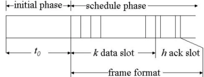
CoLaNet assumes that a single, time-slotted channel for both data and signaling transmission. Note that it is applicable for a multi-channel environment as well. Figure 1 depicts the overall time-slot organization of the CoLaNet protocol. Time is organized as a sequence of alternate initial (or contention-based) and schedule-based access periods. As stated in Section 1, in this work we consider data-collection applications for a wireless sensor network. Since the traffic for such application is many-to-one, which suggests a tree-based routing structure. Our CoLaNet uses this characteristic to construct the routing tree, which is used to gather the interested information from the sensor node back to the sink. Moreover, during the initial (or contention) period, each sensor node exchanges the signaling packets, locally select its parent node for constructing the routing-tree, and send its one-hop neighbor information back to the sink.

Figure 1: Initial phase t0 and the frame format, with

k data slots and h ack slots, in scheduled phase.

2.1 Routing-Tree Construction

At the routing-tree construction step, each sensor node needs to figure out a better way to locally select its parent node and then transmit this information as well as its one-hop neighbors back to the sink. An efficient routing tree for a wireless sensor network is expected to be able to (a) minimize the end-to-end delivery time, i.e., the sensing data could be timely delivered to the sink such that the decision maker can take immediate action to deal with that emergency event, and (b) minimize the access contention or the interference between the data transmissions, i.e., via this better routing decision, the sensor network could save more energy consumption by avoiding packet

collisions and at the same time achieve high

throughput. Furthermore, an optimal routing-tree is also a function of the topology sensor network as well as the arriving pattern of sensing events.

After receiving each node’s local information, the sink uses ``the channel assignment algorithm’’ to decide the transmission schedule (or the duty cycle) of

each sensor node. To ensure a collision-free

transmission and maximize the system capacity, our CoLaNet first transforms this channel assignment problem for a sensor net into a vertex-coloring problem in its corresponding graph. By solving the vertex-coloring problem through some well-known approximation algorithm [8], the sink is able to determine each sensor schedule and send that schedule information back to each node. From now on, each sensor node is able to transmit the interested data back to the sink according its assigned schedule.

Instead of searching for the optimal routing tree, we investigate 3 local tree-construction schemes for our CoLaNet. The first scheme is min-degree tree, i.e., each node chooses the node with fewest children nodes as its parent. Intuitively, this scheme is able to reduce the probability of contention or collision between neighboring data transmissions. The second one is nearest-first tree. In this scheme, a sensor node will choose the nearest node (or the node with the strongest signal) to be its parent node. This scheme is simple and used as a baseline for comparison only. The last one is

random tree, where each node randomly chooses its parent node from all possible candidate nodes that are one-hop closer to the sink.

2.2 Channel Assignment Algorithm

In this section, we present how to determine the schedule of a sensor node through our channel assignment algorithm.

2.2.1 Link-based Data Slot Assignment

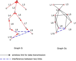
Given that a wireless sensor network has N nodes, each node is able to communicate directly with its neighboring node (within its transmission range) via wireless links. If node i, n(i), directly transmit a packet to node j, n(j), we use a directed edge (link), e(i,j), to represent it. Hence, the routing tree for collecting data packet could be represented by a directed graph G = (V, E) (as shown in Figure 3), where V is the set of nodes in the network and E is the set of directed edges (link) in the network.

An edge-coloring problem of a graph G is how to color the edges of G such that no adjacent edges have the same color. We note that any proper edge coloring of this directed graph G can be mapped into an achievable transmission schedule and vice-versa. To achieve this mapping, let us consider a scheduling

frame with slot of length ts seconds each. Each edge e

in the scheduling graph G corresponds to one time slot that has to be allocated to the link that represent edge e in the graph. We could avoid any conflict between the transmission schedules through an appropriate color assignment in G. Moreover, with Nc colors we can color all edges in G, which implies that there is a valid schedule of length Nc slots for this wireless sensor network. As a result, we have mapped a proper edge coloring of the G onto a valid transmission schedule.

However, in a wireless sensor network, two communications might interfere with each other even though they have different senders and receivers, i.e., two non-adjacent edges should not use the same color if there is interference between them. This is usually referred as the ``hidden node problem’’. To avoid the hidden node problem and construct an efficient transmission schedule for a wireless sensor network, we adjust our data channel assignment scheme as follows.

First, we construct a directed graph G to represent the routing tree. Second, to avoid the hidden node problem in the wireless communication, our scheme use the collected information during the initial phase and convert the edge-coloring problem on graph G into the vertex-coloring problem on the corresponding graph Gc. At last, we can choose a suitable

approximate algorithm to solve the vertex-coloring problem and then determine the data channel assignment for the routing tree.

We now describe how to build the corresponding graph Gc given an original graph G. We construct the corresponding graph Gc of the original graph G (as shown in Figure 3) according the following principles: (1) we add a node n(j) in the corresponding graph Gc

if there is a link ej in the original graph G, and (2) we

add a link Lij in the corresponding graph Gc if link Li and link Lj (a) have the same sending node in G, (b) share the same receiving node in G, or (c) two links interfere with each other in G. That is, if two links are coming from the same node or they are going to the same node in G, these two communications should use different time slot to delivery their data to avoid the collision. The similar reason could be applied to the last case is if two links interfere with each other, i.e., two interfering transmissions cannot use the same time slot.

What remains is how to identify if there is interference between any two communications in the routing tree. Given a node n(j), the contending set for node n(j) is defined as the set CS(j), which consists of all the nodes within the node n(j)’s transmission range. We could use the interference-determining algorithm in Figure 2 to examine all possible interfering edges (or transmission) in a graph.

1 n(i): node i in G

2 e(i,j): a transmission from n(i) to n(j) in G;

3 nc(i,j): the corresponding node of e(i,j) in Gc;

4 CS(j): the contending set of the node j; 5 for each e(i,k)  G {

6 for each e(j,l) and (i z j and k z l){ 7 If ( n(i)  CS(l) or n(j)  CS(k) ){

8 Adding an edge e between nc(i,k) and nc(j,l) in Gc;

9 }}}

Figure 2: Interference-determining algorithm After we get the graph Gc, what we would like to do is to solve a vertex-coloring problem of the graph Gc. A vertex-coloring problem is to color the vertices of a graph such that any adjoining vertices have different colors. If we can color the vertexes of the graph Gc with minimal colors, we have more chances to reuse the available wireless channels. However, given a graph the minimum graph(vertex)-coloring problem is often intractable or NP-complete problem. Since our goal is not to propose a better approximate algorithm for solving the vertex-coloring problem so we just use the algorithm in [8] for CoLaNet.

L4 L2 L1 L3 L5 L6 L7 L8 L10 L9

wireless link for data transmission interference between two links

Graph G Graph Gc L1 L2 L3 L4 L5 L6 L7 L9 L8 L10

Figure 3: the Graph G (based on the data-routing tree) and its corresponding graph Gc

N 6 N 7 N 4 N 2 N 3 S ink N 1

w ireless link for data transm ission interference betw een tw o links

(a) G raph Gd (b) G raph Gd c N 5 N 9 N 8 N 10 N 6 N 7 N 4 N 2 N 3 Sink N 1 N 5 N 9 N 8 N 10

Figure 4: Node-based ack channel assignment

2.2.2 Node-based Ack Channel Assignment

To provide a reliable transmission for CoLaNet, we introduce the ack channel after the data channel. Of course, the straightforward way to add the ack channel immediately after its data channel. However, we note that (a) in the routing tree structure a parent node (the receiving node) usually has several children nodes (the sending node), (b) the ack packet is usually small size with similar payload and it is possible to put several Ack packets into one packet and (c) the wireless multicast advantage property, which permits all nodes within communication range to receive a transmission without additional expenditure of transmitter power. Therefore, we adopt a node-based ack channel assignment scheme as shown in Figure 4, i.e., the parent node only sends out one ack packet to all its children nodes. Next, each child node can examine the ack packet to see if its data is received successfully or not. That is, we add all ack slots after the all data slots.

Given the data channel assignment and the ack channel assignment, it is easy to transform those assignments into the schedule (or the duty cycle) for each sensor node.

3. Performance Evaluation

In this section, we present the performance study of CoLaNet. All experiments are done through the simulation implemented in ns2. Each simulation is run for 400 sec and the results are averaged over 10 runs. In all the experiments, we use the same physical layer model as in [2]. More specifically, the average power consumption in transmit, receive and sleep modes is 24.75mW, 13.5mW and 0mW. The size of a signal packet in the initial phase is 128 bytes. The size of a data packet and the size of an ack packet are 512 bytes and 16 bytes respectively. The bandwidth of the wireless channel is 11Mbps.

The performance metrics used in this work are: (a) the packet-received ratio at the sink, (b) the average end-to-end delivery time of a received packet, and (c) the average power consumption of a successfully received packet. Note that we also did a performance study to compare different routing-tree constructing schemes in [7]. Due to lack of space, please refer to [7] for more detailed discussion. Since the min-degree scheme performs better than or as well as any of the other tree-constructing schemes in term of packet-received ratio, end-to-end transmission time and average power consumption, we use it to construct our routing tree when we compare CoLaNet with other MAC protocols (coupled with AODV routing protocol) in the reminder of this section.

CoLaNet vs. S-MAC

S-MAC is a contention-based channel access protocol and it uses periodic sleep intervals to conserve energy. Sleep schedules are established using SYNC packets that are exchanged once every SYNC_INTERVAL. The duty cycle determines the

length of the sleep interval. The parameter

SYNC_INTERVAL is set 10 second same as in [2] and we vary the duty cycle from 40% to 70% in this experiment.

We note that S-MAC often needs a long time to set up the listen/sleep schedule with the neighbor. To shorten the schedule-synchronized process, we favor S-MAC by considering a small-scale wireless sensor network in this experiment. We vary the total number of sensor nodes from 2 to 15, which are uniformly distributed in a 300x300m area. The data rate is 1

packet per second. In addition, in this study S-MAC is coupled with the routing protocol---AODV to deliver the interesting data from the sensor node to the sink. Since there is no need for S-MAC to use the initial phase to collect the information, to do a fair comparison, the average power consumption for a packet in CoLaNet does include the energy used

during the initial phase, where t0 is equal to 5 second.

˃ ˃ˁ˅ ˃ˁˇ ˃ˁˉ ˃ˁˋ ˄ ˄ ˅ ˆ ˇ ˈ ˉ ˊ ˋ ˌ ˄˃ ˄˄ ˄˅ ˄ˆ ˄ˇ ́̈̀˵˸̅ʳ̂˹ʳ̆˸́̆˼́˺ʳ́̂˷˸̆ ̅˸˶˸˼̉˸˷ʳ̅˴̇˼̂ ˖̂˿˴ˡ˸̇ ̆̀˴˶ʽ˲ˇ˃ʸ ̆̀˴˶ʽ˲ˈ˃ʸ ̆̀˴˶ʽ˲ˉ˃ʸ ̆̀˴˶ʽ˲ˊ˃ʸ

5(a) packet-received ratio

˃ ˄ ˅ ˆ ˇ ˈ ˉ ˄ ˅ ˆ ˇ ˈ ˉ ˊ ˋ ˌ ˄˃ ˄˄ ˄˅ ˄ˆ ˄ˇ ́̈̀˵˸̅ʳ̂˹ʳ̆˸́̆˼́˺ʳ́̂˷˸̆ ˸˅˸ʳ˷˸˿˼̉˸̅̌ʳ̇˼̀˸ʻ̆˸˶ʼ ˖̂˟˴ˡ˸̇ ̆̀˴˶ʽ˲ˇ˃ʸ ̆̀˴˶ʽ˲ˈ˃ʸ ̆̀˴˶ʽ˲ˉ˃ʸ ̆̀˴˶ʽ˲ˊ˃ʸ

5(b) end-to-end delivery time

˃ ˈ ˄˃ ˄ˈ ˅˃ ˅ˈ ˆ˃ ˄ ˅ ˆ ˇ ˈ ˉ ˊ ˋ ˌ ˄˃ ˄˄ ˄˅ ˄ˆ ˄ˇ ́̈̀˵˸̅ʳ̂˹ʳ̆˸́̆˼́˺ʳ́̂˷˸̆ ˴̉˺ˁʳ˸́˸̅˺̌ʳ˶̂́̆̈̀̃̇˼̂́ʻ̀˝ʼ ˖̂˟˴ˡ˸̇ ̆̀˴˶ʽ˲ˇ˃ʸ ̆̀˴˶ʽ˲ˈ˃ʸ ̆̀˴˶ʽ˲ˉ˃ʸ ̆̀˴˶ʽ˲ˊ˃ʸ

5(c) average power consumption per received packet Figure 5: CoLaNet vs. S-MAC

We now start out to compare CoLaNet and S-MAC. In general, the results in Fig. 5 indicate that schedule-based CoLaNet is able to achieve higher delivery ratio than contention-based S-MAC does. Such performance

improvement is mostly due to the collision-free guarantees at all times during data transmission. On the other hand, S-MAC is more susceptible to the contention or hidden terminal collisions. Therefore, as the total number of sensor node increase, the improvement becomes more significant. For instance, as shown in Fig. 5(a) for 15 sensor nodes case the received ratio of the CoLaNet (compared to S-MAC) is 1.7 times under the duty cycle of 70% S-MAC and 2.8 times under the duty cycle of 40% S-MAC.

Moreover, we note that although the CoLaNet is a schedule-based MAC, compared to S-MAC, it could also provide a lower end-to-end delivery time as depicted in Fig 5(b). This could be explained as follows. First, since our channel assignment scheme makes use of the temporal and spatial channel reuse properties to minimize the number of time slots in a super-frame, each sensor node only needs to wait a length of super-frame to access next available time slot even if it miss the current one. Second, as a packet is transmitted on the first hop, it is likely to be successfully delivered to the sink since the collision-free transmission is guaranteed in the CoLaNet. On the other hand, the contention-base MAC such as S-MAC or 802.11 might suffer the contention collision a lot when the traffic becomes heavy.

Finally, we would like to compare the CoLaNet and

S-MAC with respect to the average energy

consumption metric. As can be seen in Figure 5(c), the CoLaNet can save more energy. This, of course, is not surprising since the CoLaNet is carefully planned by considering the different characteristics of different layers and trying to satisfy each layer’s requirement.

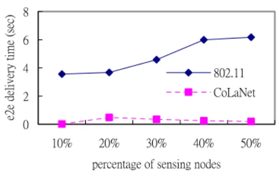
CoLaNet vs. 802.11

In this experiment, we compare our CoLaNet (t0 =

10 sec) with 802.11(+AODV) in term of packet-received ratio and end-to-end delivery time metrics. We do not evaluate 802.11 under the energy consumption metric since 802.11does not address the energy conservation. In addition, 802.11 does not need a warm-up time to settle down each sensor schedule so that we consider more sensor nodes in this experiment. There are 70 sensor nodes uniformly distributed in a 500x500m area.

Figures 6 and 7 show the corner sink case and the center sink case respectively. Qualitatively, the observation we made above, in comparing S-MAC, still hold under different traffic patterns, i.e., similar trends persist. In addition, as shown in Figure 6(a) and 7(a), both the CoLaNet and 802.11 have higher packet-received ratio under the center sink case compared to under the corner sink case. This is because the hop count from the sensor to the sink become smaller as

the sink is moved from the corner to the center. As we can see in Fig. 6(b) and Fig. 7(b), compared to the CoLaNet 802.11 is more sensitive to the location of the sink node with respect to the end-to-end delivery time metric.

Lastly, we have performed many more different traffic-pattern experiments, using various percentage of sensing nodes or sensing rates. Qualitatively, the results show similar trends as in the above Figures. Hence, we do not include all experiment results for the interest of brief. ˃ ˃ˁ˅ ˃ˁˇ ˃ˁˉ ˃ˁˋ ˄ ˄˃ʸ ˅˃ʸ ˆ˃ʸ ˇ˃ʸ ˈ˃ʸ ̃˸̅˶˸́̇˴˺˸ʳ̂˹ʳ̆˸́̆˼́˺ʳ́̂˷˸̆ ̅˸˶˸˼̉˸˷ʳ̅˴̇˼̂ ˋ˃˅ˁ˄˄ ˖̂˟˴ˡ˸̇

6(a) packet-received ratio

˃ ˄ ˅ ˆ ˇ ˈ ˉ ˊ ˋ ˄˃ʸ ˅˃ʸ ˆ˃ʸ ˇ˃ʸ ˈ˃ʸ ̃˸̅˶˸́̇˴˺˸ʳ̂˹ʳ̆˸́̆˼́˺ʳ́̂˷˸̆ ˸˅˸ʳ˷˸˿˼̉˸̅̌ʳ̇˼̀˸ʳʻ̆˸˶ʼ ˋ˃˅ˁ˄˄ ˖̂˟˴ˡ˸̇

6(b) end-to-end delivery time

Figure 6. Corner Sink Case: the data rate is 20 pkts/s

˃ ˃ˁ˅ ˃ˁˇ ˃ˁˉ ˃ˁˋ ˄ ˄˃ʸ ˅˃ʸ ˆ˃ʸ ˇ˃ʸ ˈ˃ʸ ̃˸̅˶˸́̇˴˺˸ʳ̂˹ʳ̆˸́̆˼́˺ʳ́̂˷˸̆ ̅˸˶˸˼̉˸˷ʳ̅˴̇˼̂ ˋ˃˅ˁ˄˄ ˖̂˟˴ˡ˸̇

7(a) packet-received Ratio

˃ ˅ ˇ ˉ ˋ ˄˃ʸ ˅˃ʸ ˆ˃ʸ ˇ˃ʸ ˈ˃ʸ ̃˸̅˶˸́̇˴˺˸ʳ̂˹ʳ̆˸́̆˼́˺ʳ́̂˷˸̆ ˸˅˸ʳ˷˸˿˼̉˸̅̌ʳ̇˼̀˸ʳʻ̆˸˶ʼ ˋ˃˅ˁ˄˄ ˖̂˟˴ˡ˸̇

7(b) End-to-End Delivery Time Figure 7. Center Sink Case: the data rate is 20

pkts/sec

4. Conclusions

This paper uses a cross-layer approach to design a wireless sensor network. Such cross-layer design approach is important since it is able to organize the upper layer such as the network layer or the transport layer to meet the application’s requirements and in the meanwhile uses that upper information to plan the lower layer’s, i.e., MAC layer, schedule or access control to avoid collision. As a result, this design leads to a more energy-efficient design and provide better system performance.

5. References

[1] W. Ye, J. Heidemann, and D. Estrin, "An Energy-

Efficient MAC Protocol for Wireless Sensor Networks, IEEE

INFOCOM, New York, NY, USA, June, 2002.

[2] V. Rajendran, K. Obraczka, and J.J. Garcia-Luna-Aceves,

"Energy-Efficient, Collision-Free Medium Access Control for Wireless Sensor Networks," Proc. ACM SenSys 03, Los

Angeles, California, 5-7 November 2003.

[3] Tiks Van Dam, Koen Langendoen,”An Adaptive Energy-Efficient MAC Protocol for Wireless Sensor Networks”, in ACM Sensys, Nov. 2003

[4] Xue Yang and Nitin Vaidya, “A Wakeup Scheme for

Sensor Networks: Achieving Balance Between Energy Saving and End-to-End Delay,” IEEE RTAS 2004. May, 2004.

[5] C.F. Chou, J.J. Su, and C.Y.Chen, "Straight-Line Routing

for Wireless Sensor Networks", in Proc. of IEEE ISCC,

Cartagena, Spain, Jun. 2005.

[6] Y. Sankarasubramaniam, O. B. Akan, I. F. Akyildiz, "ESRT: Event-to-Sink Reliable Transport in Wireless Sensor

Networks," in Proc. ACM MOBIHOC 2003, pp. 177-188,

Annapolis, Maryland, USA, June 2003.

[7] K. T. Chuang, “An energy-efficient wireless sensor network”, Master Thesis, Aug. 2004, CSIE dept., National Taiwan University.

[8] Skiena, S. "Edge Colorings." Implementing Discrete

Mathematics: Combinatorics and Graph Theory with Mathematica. Reading, MA: Addison-Wesley, p. 216, 1990.