Analysis of a Software Reliability Growth Model with
Logistic Testing-Effort Function
Chin-Yu Huang and Sy-Yen Kuo
Department of Electrical Engineering
National Taiwan University
Taipei, Taiwan
[email protected]
Abstract
In this paper, we investigate a S o f i a r e Reliability Growth Model (SRGM) based on the Non Homogeneous Poisson Process (NHPP) which incorporates a logistic testing-effort function. Software reliability growth models proposed in the literature incorporate the amount of
testing-effort spent on software testing which can be described by an Exponential curve, a Rayleigh curve, or a Weibull curve. However, it may not be reasonable to represent the consumption curve for testing-effort only by an Exponential, a Rayleigh or a Weibull curve in various software development environments. Therefore, we will show that a logistic testing-effort function can be expressed as a software developmenthest effort curve and give a reasonable predictive capability for the real failure data. Parameters are estimated and experiments on three actual tesddebug data sets are illustrated. The results show that the software reliability growth model with logistic testing-effort function can estimate the number of initial faults better than the model with Weibull-type consumption curve. In addition, the optimal release policy of this model based on cost-reliability criterion is discussed.
1. Introduction
A computer system consists of two major components : hardware and software. Although extensive research has been done in the area of hardware reliability, research has also been conducted to study the software reliability of computer systems since 1970. Software reliability is the probability that a given software will be
Ing-Yi Chen
Department of Electronic Engineering
Chung Yuan Christian University
ChungLi, Taiwan
functioning without failure in a given environment during a specified period of time. Hence, software reliability is a key factor in software development process and software quality. The testing phase is an important and expensive part during the software development process which includes the following four phases: specification, design, programming and test-and-debug. Many resources are consumed by a software development project. Most papers assumed that the consumption rate of testing resource expenditures during the testing phase is a constant or even do not consider such testing effort. In reality, software reliability models should be developed by incorporating different testing-effort functions. Yamada et al. [l-41 and Musa et al. [ 5 ] proposed a new and simple software reliability growth model which describes the relationship among the calendar testing, the amount of testing-effort, and the number of software errors detected. The test-effort is measured by the number of CPU hours, the number of executed test cases, and so on.
SRGMs proposed by most papers incorporate the effect of testing effort in the software reliability growth and the software development effort can be described by the traditional Rayleigh, Weibull or Exponential curve. However, in many software testing environments it is
difficult to describe the testing-effort function by the above three consumption curves. In this paper, we thus
will show that a logistic testing-effort function can be expressed as a software developmentitest effort curve. Experiments have been performed based on three real testidebug data sets. The results show that the SRGMs with a logistic testing-effort function can estimate the number of initial faults better than previous approaches.
1.
2.3 .
4.
5.
6. --The error removal process follows the Non
Homogeneous Poisson Process (NHPP).
The software system is subject to failures at random times caused by errors remaining in the system.
The mean number of errors detected in the time interval (t, t+At] by the current test-effort is
proportional to the mean number of remaining errors in the system.
The proportionality is a constant over time. The consumption curve of testing effort is modeled by a logistic testing-effort function. Each time a failure occurs, the error which caused it is immediately removed, and no new errors are introduced.
This paper is divided into six sections. Section 2 gives a brief description of some testing-effort functions already published in the literature and the Logistic testing-effort function. Section 3 investigates the software reliability growth model with the logistic testing-effort function. We estimate the parameters of this SRGM with the logistic testing-effort h c t i o n by using the least square method, apply this model to actual software failure data, and show numerical illustrations in Section 4. Section 5 is concerned with applications of this model on the optimal release policy based on the cost-reliability criterion. Finally, Section 6 concludes this paper.
2. Testing-effort functions
2.1 Review of traditional testing-effort functions In this section, we will briefly review some testing -effort functions. During software testing phase, it consumes much test-effort, such as man power, number of test cases, and CPU time. Traditionally, the test-effort during the testing phase and the time-dependent behavior of development effort in the software development process can be described by an Exponential, a Rayleigh or a Weibull curve, which were proposed by Yamada et al. [ I , 2, 3,4], Musa et al. [5], Putnam [6] and Kapur et al. [7, 81.
Let W(t) be the cumulative amount of testing-effort
expenditures in the testing time interval (0, t ] and g(t) be the consumption rate of the testing effort expenditures. Thus, the testing-effort consumed per unit time is assumed to the proportional to the remaining amount of the testing-effort expenditures a - W(t). Following the
general assumptions [3, 41, we can get the differential equation [ 1, 31:
Solving the above equation, we get
(-j;
g C M ) ]W(t) =
a
x [ 1-
eand W(t) is defined as fcillow:
where c1 is the total amount of testing effort to be
eventually consumed, g(t) is the consumption rate of testing-effort expenditures and w(t) is the current testing effort consumption at tirne t [ 3 ] .
1.
If g(t) =p,
then w(t)= ap exp[-pt1,
we have an Exponential curve and the integral forms ofw(t) (i.e. the cumulative testing-effort consumed in time (0, t] ) is W(t)=a(l- exp[-Pt]).
P
2.
If g(t) = Pt, then w(t)= apt exp[-Tt2 ] and we have a Rayleigh curve and the integral forms ofP
w(t) is W(t)=a(l- exp[-Tt2 1).
3.
And if w(t)=cc.pm tm-' exp[-pt"1,
we have a Weibull Curve and the integral forms of w(t) iswhere
P
is the scale parameter and m is the shape parameter.(4)
( 5 )
W(t)=a( 1-exp[ -pt" ] ), (6)
In the Weibull-type c;urves (i.e. Eq. (6)), when m=l or m=2, we obtain the exponential or the Rayleigh curve respectively and they are the special cases of the Weibull testing-effort function. In the Weibull-type curves, when m=3, 4, and 5, we can find that these testing-effort curves almost have an apparent peak Phenomenon (i.e. non-smoothly increasing and degrading consumption curve ) during the software development process. That is, an extreme peak work rate will occur. This phenomenon seems not so realistic because it is not commonly used to interpret the actual software developmenthest process. It sometimes may not be suitable for modeling the test effort consumption curve although the Weibull function can be made to fit or approximate many distributions and represents flexible testing effort by controlling the shape parameter m. General speaking, from our study [l-4, 7, 81, the estimated value of m usually will not be larger than 2.5 in many real world applications
.
2.2 Logistic testing-effort function
Since actual testing-effort data express various expenditure patterns, sometimes the testing-effort expenditures are difficult to be described by only a Exponential or Rayleigh curve. Although the Weibull -type curve can fit the data well under the general software development environment, it will have an apparent peak phenomenon when the shape parameter m>3. Therefore, we try to use a logistic testing-effort function which was first presented by Parr [9] instead of the Weibull type testing-effort consumption function as the testing-effort function to describe the test effort patterns during the software development process. This obtained function differs from the Weibull-type function described in the above subsection and was used to derive the form of the resource consumption curve of a project over its life cycle [9]. The logistic testing-effort function has the following form:
The cumulative testing effort consumption in time (0, t] is
W(4 = N (7)
and the current testing effort consumption
( 8 ) d w ) ah"*
(1 +A@')
w(t) = = ~
where N is the total amount of testing effort to be eventually consumed, a is the consumption rate of testing-effort expenditures, and A is a constant. Therefore,
) is a smooth bell-shaped we can see that w(t) (=-
( I + A e*)2
function. The testing effort w(t) reaches its maximum value at time
aAN e-U'
(9)
1 tmax = a 1nA
Compared with the Weibull-type testing-effort function in the starting point, the value of logistic testing-effort function W(0) is non-zero. The divergence between the Weibull-type curve and W(t) is concentrated in the earlier stages of software development where progress is often least visible and formal accounting procedures for recording the amount of testing effort applied may not have been instituted. It is possible for us to judge between these models using some statistical test of their relative ability to fit actual failure data, such as adjusting the origin and scales linearly [9].
3. Software reliability growth model
Based on the assumptions, if the number of detected errors due to the current testing-effort expenditures is
proportional to the number of remaining errors, then we obtain the following differential equation [3]:
where m(t)=the expected mean number of errors detected in time (0, t]
w(t)= current testing effort consumption at time t a = the expected number of initial faults
r = error detection rate per unit testing-effort at testing Solving the above differential equation under the boundary conditions m(O)=O (i.e., the mean value function m(t) must be equal to zero at time 0), we have
time t that satisfies 00.
m(t)=a( 1- exp[-r (W(t)-W(0) ) ] ) (1 1) =a( 1- exp[-r W*(t) ] )
Substituting Eq. (12) into Eq. (1 l), we obtain m(t)=a(l- N - )
3
) and the failure intensity function (or instantaneous error detection rate) h ( t ) e =anu(t) exp[-rW*(t)1.
exp [-' ( 1 +A exp (-at) 1 +A
The expected number of errors to be detected eventually is m(") = a(1- exp[-r
E
3
). If A >> 1, then m(co) za(1- exp[-r N] ). It represents the expected number of undetected errors after an infinite test time a-m(" ) = = a x e x p [ - r E ] G a x exp[-rl\il. Hence, all the original errors in a software system can't be hlly detected after a long time because the total amount of testing effort to be eventually consumed during the testing phase is limited to
N . It requires an infinitely large amount of testing effort if all errors are to be testedremoved which is almost impossible because the test team can not devote all their efforts and resources on a software product forever. The test team has to release a software to market at the righthest time taking into the economic considerations.
4.
Numerical examples4.1 Estimation of model parameters by least square method
To validate the proposed Software Reliability Growth Model with a logistic testing-effort function in Eq.( 1 l),
performed. Two most popular estimation techniques are
Miximum Likelihood Estimation (MLE) and Least Squares Estimation (LSE) [5, 9, 10, 191. The method of least squares minimizes the sum of squares of the deviations between what we actually observelget and what we expect and the least squares estimation provides the best point estimates [lo]. Therefore, we decided to fit the logistic curve and the proposed model directly on the above three data sets, using the least sum of squares criterion to give a "best fit". That is, the parameters N , A, and c1 of the logistic testing function in Eq. (7) and the parameters a, r given in Eq. (1 1) can be estimated by the method of least squares. In the method of least square sum, the evaluation formula SI(N, A, a) and S2(a, r ) are as follow:
where W, is the cumulative testing effort really consumed in time (0, tJ and W(t,)is the cumulative testing effort estimated by the logistic testing function in ( 7 ) . The mk is the cumulative number of detected errors in a given time interval (0, tk] and m(fJ is the estimated cumulative
number of detected errors in (1 1). Differentiating SI (S2) with respect to N , A, and c1 (a, r ) , setting the partial derivatives equal to zero and rearranging these terms, we can solve such kind of nonlinear least square problems. For example, consider the Logistic testing effort function and take the partial derivatives of SI with respect to N , A and a. First we get
Thus, the least squares estimator N is given by solving the above equation:
The other parameters A and a can also be solved by substituting the least squares estimator N into Eq. (17)
and (1 8). Besides, we choose two comparison criteria of estimation described as follow:
(1) The Accuracy of Estimation [5, 1 1, 181
(AE)=
lyl
(19)where M, is the actual cumulative number of detected errors during the test and after the test, and m is the estimated parameter a :in Eq. (1 1).
(2) The Mean of Square fitting Errors
c
[m(tk)-mkl'k (MSE)= '='
The lower MSE indicates less fitting errors and better performance [ 81.
4.2
Fitting model to real software data and data analysisFirst Data Set
The first set of real data is from a study by Ohba [12]. The system is a PLO database application software consisting of approximately 1,3 17,000 lines of code. During nineteen weeks, 47.65 CPU times were consumed and about 328 software errors were removed. Besides, the total cumulative number of detected faults after a long time of testing is 358 [ 11, 121. In order to estimate the parameters N , A, and a of the logistic testing function, we fit the actual testing-effort data into Eq. (13) and solve it by using the method of least squares. These estimated parameters are:
N=54.8364, A=13.0334., a=0.226337.
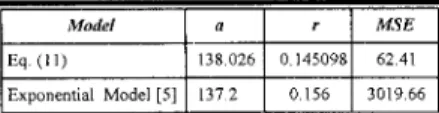
The above parameters of testing effort function and the actual software error data are applied to Eq. (14). The other parameters a, ,r in (1 1) can also be solved numerically by the method of least squares for these failure data. Table 1 shows the estimated parameters of Eq.(l 1) and compares with the estimated initial faults m and MSE of other general models. Fig. l(a), Fig. 1 (b) and Fig. l(c) graphically illustrate the fitting of the estimated current testing effort by using Eq. (8), Weibull function and Rayleigh function respectively. The cumulative numbers of estimated failures by Eq. (1 1) are:
~ 3 9 4 . 0 7 6 , ~ 0 . 0 4 2 7 2 2 3
In addition, substituting the estimated parameters A and a in Eq.(9), the testing effort function reaches the maximum at time ~ 1 1 . 3 4 3 8 weeks which corresponds to
w(t)=3.10288 CPU hours and W(t)=23.5107 CPU hours. Besides, the number of c:rrors removed up to this time t,,,,
is 245.421. Fig. l(d) shows the actual (observed) and fitted software failures versus test time. From the fit in
Fig. l(a) and the comparison criteria in Table 1, we see that the fit in Fig. l(a) is better than that in Fig. l(b) and Fib. (c). Hence, we can conclude that a SRGM with Logistic testing-effort function gives a better fit in this experiment .
Table 1. Comparison results for the first data set.
I I I I
3 9 4 0 7 6 00427223 1 0 0 6 11829
c..n M ~r I I 1 ~ ~ I I 5 6 2 8 I * I 5 6 9 8 I 15775
Eq (11)
Inflection S-Shaped Model [I21 I 389 I 10 0935493 I 8 69 I I33 53 11
1
I
Loearithmic Poisson Model I I I 1 not exist1353 2
1
1
1
I:1
2 9 0 6 9 1Delayed S-ShapedModel [ I l l
Exponential Model [ 121 455 37 00267368 2 7 0 9 2 0 6 9 3
Eq ( I O ) with Weibull function 565 35 0 0196597 57 91 122 09
Eq (10) with Rayleigh function 459 08 0 0273367 28 23 268 42 171 23
a = expected initial faults
r = error detection rate per unit testing effort
Testing Effort (CPU Hours)
O w
-I Time ( W e e k s )
0 2 . 5 5 7 . 5 10 12.5 15 17.5
Figure 1 (a). Observedlestimated current testing -effort by using logistic function vs. time.
Testlng Effort(CPU HOUTS)
Tlme(weeks1
Figure 1 (b). Observed/estimated current testing -effort by using weibull function vs. time.
Tescing EfforciCPU Hours)
0 2 . 5 5 7.5 10 12.5
Figure 1 (c). Observedlestimated current testing -effort by using rayleigh function vs. time.
0 5 10 15 20
Time (weeks)
Figure l(d). Cumulative number of observed /estimated failures vs. time.
Second Data Set
The second set of real data is the pattern of discovery of errors in the software that supported Space Shuttle flights STS2, STS3, STS4 at the Johnson Space Center. The system is also a real-time command and control application [13]. A weekly summary of software test hours and the errors of various severity discovered is
given in [13]. The cumulative number of discovered faults up to thirty-eight weeks is 227. Following the same procedure described in First Data Set, the testing-effort data are applied to estimate the parameters
N,
A, and a of the logistic testing function described in Eq. (13) by using the method of lease squares. These estimated parameters are :N=2828.88, A=l0.5057, a=0.0988842
The above parameters of testing effort function and the actual software error data are applied to Eq. (14). The other parameters a, r in ( 1 1 ) can be solved numerically by the method of least squares for these failure data:
In addition, substituting the estimated parameters A and
a
in Eq. (9), the testing effort function reaches the maximum at time ~ 2 3 . 7 8 4 6 weeks which corresponds to w(t)=69.9329 CPU hours and W(t)=1168.57 CPU hours. Besides, the number of errors removed up to this time t,,),is 154.672. Table 2 shows the estimated parameters of Eq. (1 1) and compares with the estimated initial faults m and MSE of other general models. Fig. 2(a) and Fig. 2(b) plot the fitting of the estimated current testing effort by using Eq. (8) and the Rayleigh function respectively. Fig. 2(c) shows the actual (observed) and fitted software failures versus test time. From Fig. 2(a), Fig. 2(b) and Table 2, we know that the SRGM with Logistic testing effort function fits the second data set better than others in this experiment.
Table 2. Comparison results for the second data set.
Model
-0 Model [ 131
15041 21 ~ a = expected initial faults
r = error detection rate per unit testing effort
Testing Effort(CPU Hours)
0 10 20 30
Time (Weeks)
Figure 2(a). Observed/estimated current testing -effort by using logistic function vs. time.
Testing Effort(CPU Hours)
Time(Weeks)
0 10 2 0 3 0
Figure 2(b). Obsenred/estimated current testing -effort by using rayleigh function vs. time.
0 10 20 30 40
Time (weeks)
Figure 2(c). Cumulative number of observed /estimated failures vs. time.
Third Data Set
The third set of real data in this paper is the System T1 data of the Rome Air Development Center (RADC) projects in [ 141 and the failure data is generally of the best quality. The system T1 is used for a real-time command and control application. In this case, the size of the software is approximately 2 1,700 object instructions. It took twenty-one weeks and nine programmers to complete the test. During the test phase, about 25.3 CPU hours were consumed and 136 software errors were removed [ 141.
First, we still will estimate the parameters N, A, and a of the logistic testing function in (13) by using the method of least squares. These estimated parameters are : N=29.1095, A=4624.89, a=0.493515.
The above parameters of testing effort function and the actual software error data are applied to Eq. (14). The other parameters a, r in Eq. (1 1) can be solved numerically by the method of least squares for these failure data:
a= 1 3 8.1 65, r=O. 145098
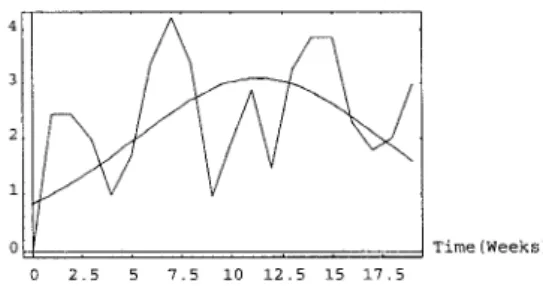
In addition, substituting the estimated parameters A and a in Eq.(9), the testing effort function reaches the maximum at time t=17.1002 weeks which corresponds to w(t)=3.59149 CPU hours and W(t)=14.5484 CPU hours. Besides, the number of errors removed up to this time t,,,, is 121.343. The fit in Fig. 3(a) appears to be good. Table
3 and Fig. 3(b) show the data analysis, and the actual(observed) and fitted software failures versus test time respectively.
5.
Optimal release policy
5.1 Software Release Time based on Reliability Criterion
In general, the software release time problem is associated with the reliability of software system. First we discuss the release policy based on the reliability criterion. If we know that the software reliability of this computer system has reached an acceptable reliability level, then we can determine when to release this software Table 3. at the right time. Okumoto and Goel [ 151 first dealed with the release problem considering the software cost-benefit. Comparison results for the third data set'
The conditional reliability function after the last failure occurs at time t is obtained by
R ( f
+
Atlt) = exp(-[m(t+ At) - m(t)])a = expected initial faults
r = error detection rate per unit testing effort = exp(-m(At) x exp(-rW*(t))) (21)
Testing Effort(CPU Hours) Taking the logarithm on both sides of the above equation
and rearranging the above equivalent, we obtain
0 5 10 1 5 2 0
Figure 3(a). Observed/estimated current testing -effort by using logistic function vs. time.
1401
2
S
100.
i t i /i/-*+-
1
+i' / " , , ,1
0 ' 3 0 5 10 15 20 25 Time (weeks)Figure 3(b). Cumulative number of observed /estimated failures vs. time.
(22) In R = -m(At) x exp(-rW*(t))
Thus, W *(t)=
+[
lnm(At) - In Ini]
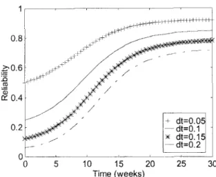
(23) Solving Eq. (22) and Eq. (12) we can calculate that the testing time needed to reach a desired reliability R. For example, we discuss the first real data set described in subsection 4-2. In First Data Set, N=54.8364, A=13.0334, a=0.226337, a=394.076 and r=0.0427223. Suppose this software system is desired that this testing would be continued till the operational reliability is equal to 0.8 (at dt=O.l), From Eq. (23) and Eq. (12), we get F19.1221 weeks. If the desired reliability is 0.85, then ~ 3 1 . 0 5 9 3 weeks (refer to Fig. 4). Similarly, in Second Data Set, N=2828.88, A=10.5057, a=0.0988842, a=241.325 and r=0.000907329. Suppose this software system is desired that this testing would be continued till the operational reliability is equal to 0.9 (at AFO. l), From Eq. (23) and Eq. (12), we get t=31.5848 weeks. If the desired reliability is 0.92 (0.95), then ~ 3 6 . 2 8 9 3 (57.1049) weeks.I \ I
Case 2 : if T 3 0 0 , thenw(m)=N, m ( m ) =a(l - e - = ) ,
I ,
-
7
> d
0 5 10 1 5 20 25 30
Time (weeks)
Figure 4. Plots of reliability of first data set versus timeforAt=0.05,0.1,0.15and0.2.
5.2 Optimal release time based on cost-reliability criterion
In this section, we will discuss the cost model and release policy based on the cost-reliability criterion. Using the total software cost evaluated by cost criterion, the cost of testing-effort expenditures during software testingidevelopment phase and the cost of fixing errors before and after release are [2, 16, 17,201:
where T,,=software life-cycle length
Cl=cost of fixing an error during testing C2=cost of fixing an error during operation C3=cost of testing per unit time
( C 2 X l )
Differentiating the above equation with respect to T and setting it to zero, we obtain
h(7) w(7)
Case 1: if T=O, then m(O)=O, - = ar,
A(7) .
Therefor, we can know that
-
1s monotonicallyw(?l A(1) (‘3 (‘3 W) w(0) C2-C,, then - 5 ~ decreasing in T. If - = ar I - W(f) C2-c1 w(o)(= ar) > (.2-c.1 w(7)
for 0 < T < TL(. . Hence, for this case, the optimal
software release time T*=O. If
(‘3 > - ( = a r e - = ) , there exists a finite
and unique solution To s,atisfying
r,\ -1
i3
-
W)Rearranging the above equation, we obtain
(27) To = U 1 x In(%) minimizes C(T)
0 < T < To and m7)
7
> 0 for T > T o , the minimum of C(7)C2-C1 N dc‘( 1)
where 0 = + ( l n ( u r r ) )
+
1 + ~
.
is at T =TO
for To 5 T .Because
7
< 0 forFrom subsection 5- I , we can easily get the required testing time needed to reach the reliability objective R,. Here our goal is to minimize the total software cost under the consideration of desired software reliability and then the optimal software release time is obtained. That is, we can mathematically minimize C(7) subject to R(t+Atlt) 2 R, where O<R,,<l [2, 16, 17,201.
T* = optimal software release time or total testing time where To = finite and unilque solution Tsatisfying Eq. (24)
= max{T,, TI}
TI = finite and unique T satisfying ~ ( t + t ) = R~
(0 < Ro < 1)
Theorem I :
Assume C1>0, C2>0, C3>0, C 2 X 1 , Dt>O, O<R,<l, we have
then T*= max{To, 1;) for R(AtlO)<R,<l or I*=To for O<R,<R(AtlO)
2. if - <
-?-
then T*=T, for R(AtIO)<R,<l or T*=O w(0) - (2-CIfor O<R,IR(AtlO) h(O) ( 3
3. if ~ ( 0 ) 2
c2-c’1
then T * L T I for R(AtjO)<R,<I or T* 2 0 for O<R,rR(AtlO)In order to illustrate the above derivation, we consider the three real data set described in the previous section and use them to work as numerical examples on the optimal software release problem.
Discussions:
1) First Data Set: From the previous estimated parameters: we know N=54.8364, A=13.0334, a=0.226337, ~ 3 9 4 . 0 7 6 , r=0.0427223 and assume Cl=IO, C2=50, C3=100, TL,=lOO, R, =0.85, AFO.1. Then we get the optimal release time To estimated as 20.3753 based on minimizing C(T) of Eq. (24) and TI estimated as 3 1 .OS93 based on satisfying the reliability
V O ) c3
criterion of R(t+Atlt)=R,. Moreover, since - N O ) >
e
,
c3 and R(At/0)=0.2481<R0, T*= max
W(
n
c2-c1(20.3753, 3 1.0593}=3 1.0593 weeks. The optimal total software cost C(T*)=8572.21 (plot is given in Fig. 5) and the achieved software reliability R(3 I.O593+At(=O. 1) 13 1.0593) is 0.85. rNA
-_
ho
= are l+A <-
T o t a l S o f t w a r e C o s t 15000 50001
2 5 0 0 ' 0 T i m e (Weeks) 1 0 2 0 30 40 5 0Figure 5. Total software cost of the first data set vs. time.
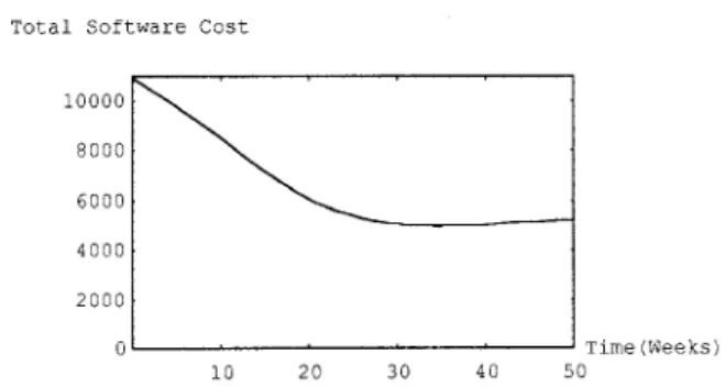
2) Second Data Set: From the previous estimated parameters: we know N=2828.88, A=10.5057, a=0.0988842, a=241.325, r=0.000907329 and assume C I = l , C2=50, C3=2, T,,=200, R, =0.95, AtZ0.1. Then we get the optimal release time To estimated as 34.4345 based on minimizing C(T) of Equation (24) and TI estimated as 57.01049 based on satisfying the reliability criterion of R(t+Atlt)=R,. Since
9
> &!-are '+A i
-
c2-r1 and R(AtIO)<R,, Tc=max{34.4345,57.01049 }=57.01049. The optimal total software cost C(T*)=5290.2 (see Fig. 6) and the achieved software reliability is R(57.0 1049+At(=O. 1)157.0 1049)=0.95 . = w(0) c2-c1 ' w(7)
_-
+U C3 T o t a l S o f t w a r e C o s t 2000 4000I
01 I Time (Weeks) 10 2 0 30 40 50Figure 6. Total software cost of the second data set vs. time.
3) Third Data Set: From the previous estimated parameters: we h o w N=29.1095, A=4624.89, a=O.493515, a=138.165, r=0.145098 a n d assume C1 = I , C2=100, C3=50, TLc=lOO, R, =0.95, A t = ] . Then we get the optimal release time To estimated as 20.9839 based on minimizing C(T) of Equation (24) and T, estimated as 12.7957 based on satisfying the reliability criterion of
and R(AtlO)<R,, T* is estimated as max(20.9839, 12.7957)=20.9839. The optimal total software cost C(T*)=1329.44 (plot is shown in Fig. 7).
rNA
U O ) > Q
ho
= < R('+Atlr)=R,. Because ~ ( 0 ) c2-c. , w(?3c2-CI
Total Software Cost
\
6000 4 o o o j 2000: 0 i-_- T i m e ( W e e k s ) 10 2 0 3 0 4 0 50Figure 7. Total software cost of the third data set vs. time.
6. Conclusions
In this paper, we have proposed a Software Reliability Growth Model which incorporates a logistic testing-effort function and the testing effort consumption curve is different from the weibull-type curve used in fitting real date set. Due to incorporating the logistic testing-effort function and comparing it with the model proposed in
fits the real project data fairly well and it could give us a reasonable description of resource consumption behavior. Experimental results obtained are in close accord with the real data. In fact, the derivation of logistic testing-effort function in the original basic concepts already incorporates the human factors into consideration. Besides, the optimal release times of this model based on cost-reliability criterion are also illustrated by numerical examples.
Here, some consequences and future works are as follow:
1.
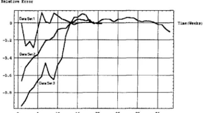
The capability of the model to predict failure behavior from present and past failure behavior is called predictive validity. Following the work in [5] and using the real project failure data described in subsection 4-2, we can compute the relative error in prediction for the three data set at the end of testing as 0.0075, -0.106, and -0.00958 respectively (see Fig. 8). From the computation results, we see that the relative errors of the first and the third data set approach zero which indicate that our model provides an accurate estimation for these data set and the relative error of the second data set is negative which indicate that the model tends to underestimate the failure phenomenon under this testing. However, the above statements imply that our model still have better predictive validity based on real failures experienced and give a more accurate prediction. That is, the software reliability growth model with logistic testing-effort function will yield the better predictions for other reliability metrics [5,19,21-231.
2 .
Although we have demonstrated that the Logistic testing-effort function is applicable to the GO model and the combined model estimate the number of initial faults better than the model with Weibull-type consumption curve, only the GO model is not sufficient to prove the applicability of the proposed Logistic testing -effort function. Presently, we are investigating how to integrate the new testing-effort function into conventional software reliability models, such as Logarithmic Poisson Model, Inflection S-Shaped Model or Delayed S-Shaped Model, and so on. If the research results fit the real failure data well, we can conclude that the Logistic testing-effort function is superior and give a more accurate descriptiodestimation for the resource consumption during software development process.0 5 10 15 20 25 30 35
Figure 8. Relative error curve for different data set.
Acknowledgment
We would like to express our gratitude for the support of the National Science Council, Taiwan, R.O.C., under Grant NSC 86-22 13-E259-002. Referees' helpful comments and suggestionis are also highly appreciated.
References
[ 11 S. Yamada, H. Ohtera, and H. Narihisa, "Software reliability growth models with testing effort", IEEE Trans. on
Reliability, vol. R-35, NID. 1, pp. 19-23, April 1986.
[2] S. Yamada, J. Hishitani, and S. Osaki, "Software Reliability Growth Model with Weibull Testing Effort : A Model and Application", IEEE Trms. on Reliability, Vol. R-42, pp.. [3] S. Yamada, and H. Ohtera, "Software Reliability Growth Models for Testing Effort Control, " European Journal of
Operational Research, pp. 343-349, 1990.
[4] S. Yamada, H. Ohtera, and H. Narihisa, "A Testing-Effort Dependent Software Reliability Model and Its application, "
Microelectronics and Reliability, Vol. 27, NO. 3, pp. [5] J. D. Musa, A. Iannino, and K. Okumoto (1987). Software Reliability, Measurement, Prediction and Application. McGraw Hill.
[6] L.H. Putnam, "A General Empirical Solution to The Macro Software Sizing and Estimating Problem, " IEEE Trans. on
Software Engineering, Vol. 4, pp. 345-367, 1978.
Imperfect Debugging Phenomenon with Testing Effort," Proceedings of the 5th International Symposium on Software Reliability Engineering, pp. 178-1 83, November 1994, Monterey, California,
Imperfect Debugging Phenomenon in Software Reliability ," Microelectronics and Reliability, Vol. 36, pp. 645-650,
1996.
100-105, 1993.
507-522, 1987.
171 P. K. Kapur. and S. Younes, " Modeling an
[9] F. N. Parr, "An Altemative to the Rayleigh Curve for Software Development Effort," IEEE Trans. on Software
Engineering, SE-6, pp. 291-296, 1980.
[IO] A. Wood, "Predicting Software Reliability, "IEEE Software,
[ 1 I] R. H. Hou, S. Y. Kuo, and Y. P. Chang, "Applying Various Learning Curves to Hyper-Geometric Distribution Software Reliability Growth Model," Proceedings of the 5th International Symposium on Software Reliability Engineering, pp. 7-1 6, November 1994, Monterey, California.
[ 121 M. Ohba, "Software reliability analysis models, " IBM J.
Res. Develop,, Vol. 28, No. 4, pp. 428-443, July 1984.
[ 131 P. N. Misra, "Software Reliability Analysis," IBM Systems Journal, Vol. 22, No. 3, pp. 262-279, 1983.
[ 141 J . D. Musa, Software Reliability Data, report and data base available from Data and Analysis Center for Software, Rome Air Development Center, Rome, NY.
[ 151 K. Okumoto and A. L. Goel, "Optimum Release Time for Software Systems Based on Reliability and Cost Criteria", J. System Software, Vol. I , pp. 315-318, 1980.
[ 161 S. Yamada and S. Osaki, "Cost-Reliability Optimal Release Policies for Software systems", IEEE Trans. on Reliability,
[I71 P. K. Kapur and R. B. Garg, "Cost reliability Optimum Release Policies for a Software System under Penalty Cost",
Int. J. of Systems Science, Vol. 20, pp. 2547-2562, 1989. error
detection rate model for software reliability and other performance measures," IEEE Trans. on Reliability, Vol.
[ 191 M. R. Lyu (1996). Handbook of Software Reliability Engineering. McGraw Hill.
[20] P. K. Kapur and R. B. Garg, "Cost-Reliability Optimum Release Policies for a Software System with Testing Effort,"
[21] S. Yamada, J. Hishitani, and S. Osaki, "Software Reliability Growth Modeling: Models and Applications", IEEE Trans. on Software Engineering, Vol. SE-I I , No. 12, pp.1431
[22] P. K. Kapur and R. B. Garg, "A software reliability growth model for an error removal phenomenon, " Software
Engineering Journal, pp. 291 -294, 1992.
[23] Xie, M., Software Reliability Modeling, World Scientific Publishing Company, 1991.
NOV. 1996, pp. 69-77.
Vol. 34, NO. 5, pp. 422-424, 1985.
[ 181 A. L. Goel and K. Okumoto, "Time dependent
R-28, NO. 3, pp. 206-21 1, 1979.
OPSEARCH, Vol. 27, NO. 2, pp. 109-1 16, 1990.