Efficiency Va~lidation of Fuzzy Domain Theories Using a Neural Network Model
Knowledge-Based Set (KBNN/TFS) is a handles trapezoidal rule revision, verific KBNN/TFS, an eficievlcy evaluate the rule Besides, three methods fuzzy rule-based neu,*aI
enhance the inference the first method, is p modifiing the antecedwts eliminate the don't care method, named transitive combines the rules wi,'h the computational lotid called identical antecedent redundant antecedents antecedents of the rules By these methods, the without changing the eficiency validation the results of performing methods. Also the ef$ciency is enhanced efficiency enhancing
Hahn-Ming Lee, Jyh-Ming Chen and En-Chieh Chang Department of Electronic Engineering
National Taiwan University of Science and Technology Taipei 106, Taiwan
[email protected]. edu. tw
Abstract
Ne>iral Network with Trapezoidal Fuzzy fuzzy neural network model, which
$izzy inputs with the abilities of fuzzy ation and generation. Based on
validation method is proposed to inference complexity on KBNN/TFS.
that simpli$ the structure of this network model are provided to eficiency. Fuzzy tabulation method, zrformed to do rule combination by of some spec@ rules and then to variables in the rules. The second fuzzy rule compacting method, the transitive relations to decrease of inference. The third method, unihing method, simpllJies the of rules by replacing the identical with a single speciJic antecedent.
structure of rules can be simpliJied results of its inference. The proposed method is used to analyze and support these three eficiency enhancing simulation results show that the aJer performing these three methods.
During the deve combine the techniqux and expert systems, employed to assure the Verification refers to implemented, and accuracy and efficiemy Efficiency validation perform a correct
1. Introduction ~
lopment stage of the models that of fuzzy theory, neural networks verification and validation should be quality of the constructed system [ 11.
assuring that the system was corrected validation does to determine whether the of the system are acceptable [2].
concerns how fast the system can infttrence for a question and how much
computer memory is required to finish the work [2]. When we find that the result of efficiency validation is unacceptable, one way we might begin to consider is to simplify the structure of knowledge. Therefore, according to the structure of rules, a general efficiency valildation method that calculates the computational load of infkrence is proposed in this paper. By this method, we c m exactly evaluate the computational load of the constructed inkrence model and measure how much the efficiency of the system is improved when it is enhanced. Furthermore, three methods that simplify the structure of the rule-constructed :neural network model are provided to enhance its inference efficiency. The three proposed methods refine the fuzzy rules in the knowledge base, and thus increase the spleed of inference. It is easy to analysis the result of performing these three efficiency enhancing methods by the proposed validation method.
2. KBNNRFS (Knowledge-Based Neural Network with Trapezoidal Fuzzy Set)
2.1 Trapezoidal LR-type fuzzy input
In KBNN/TFS, the trapezoidal LR-fuzzy interval [3]
[4], a special case of LR-fuzzy number, is used to represent the linguistic properties of fuzzy input variables and fuzzy weights. By this representation, various types of information can be described flexibly, such as linguistic, interval and numeric values. Besides, the computational load needed is not heavy.
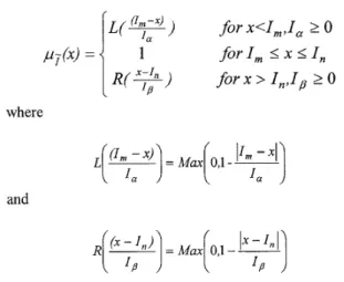
The trapezoidal LR-fuzzy interval, as shown in Fig. 1, can be denoted as T = ( I , , , , I " , I ~ , I ~ ) . I, and I,, zre the mean values and the membership degree between [ I, , I, ] is 1. I, and Ig are the left and right spreads, respectively.
The membership fimction of the LR-type fizzy interval is defined as [3]:
where
and
To measure similarity degree of two trapezoidal LR- type fuzzy intervals, a simple formula is used. We use function Similarity@, , F2) to calculate the similarity degree of Fl and F2. It is expressed as:
S u " c ~ @ ( ~ , , F2) = M a ~ J 1 - p , (Fm1-FmJ2-p, . (Fn1-F,2)2 (1)
- (FaI-Fa2) 2-(Fp,-Fp,)2, 01 The function mentioned above is based on the Euclidean distance between two fuzzy numbers. It is simple and differentiable. The output range of function Similarity is [0, 11. Besides, to reflect the different importance between mean value and spreads of a fuzzy number, parameter p1 is introduced and is set to 1.5 [5].
IP
Fig. 1. A trapezoidal LR-type fuzzy interval I" = ( i m , i n , i a , i f l )
2.2 System architecture
The initial structure of " N / T F S is constructed by existing incomplete or maybe incorrect fuzzy rules which are in Horn-clause format [ 6 ] . To translate fuzzy rules to KBNN/TFS, the S-neurons and G-neurons are used. The S-neurons calculate the firing degree of fuzzy rules, whereas G-neurons derive the consequents. Each input connection of S-neurons represents an antecedent of a fuzzy rule. That is, each antecedent is represented by a connection with fuzzy weight. Hence, a fkzzy rule's antecedents are
composed of all input connections of an S-neuron. For each consequent variable of the rules, a G-neuron is used to represent it.
3. Efficiency validation of fuzzy rules
Here, we propose a method to evaluate the efficiency of this kind of inference machines by measuring their computational load. To get the total computational load of an inference machine, we sum up the computational loads of all the conjunction operations, disjunction operations and matching operations in the model. The computational loads of a conjunction and a disjunction operation depend on the number of their inputs. To measure the computational load of an operation via the number of its inputs, we assume that each time an input is included to the operation, its computational load increased is the same. Thus, the computational load of these operations can then be treated as the combination of two terms: the constant term and the added term. The constant term is the computational load that does not change due to the number of its inputs. It can be gotten by measuring the computational load of the operation with one input. The added term increases due to the number of inputs of the operation. Suppose there is an operation with n inputs. The added term can be calculated by n-1 times the computational load increased as a new input is included to the operation. Thus, the computational load of jth conjunction operation ( Conj-CL,) and that of kth disjunction operation ( Disj -CL k) can be similarly expressed as follows:
Conj - CL = Cconj - CL + (Conj - NI - 1) * Aconj - CL ( 2 ) Disj - CLk = Cdisj - CL + (Disj - NIk -- 1) * Adisj - CL (3) where Conj-NI, indicates the number of inputs to the jth conjunction operation, and so as Disj- NIk does to the kth disjunction operation. Cconj - CL, Cdisj - CL , Aconj - CL and Adsj-CL represent the constant terms and the added terms of the computational loads of conjunction and disjunction operations, respectively.
According to equations (2) and (3), we can compute the total computational loads of all conjunction operations and disjunction operations, denoted as Conj-C&o,, and Disj-CLTotOr , in the inference machine. They can be derived as:
NCO"
,=I
= Ckconj-CL+(Conj-NI, -l)*Aconj-CL}
(4)
( 5 ) \,
as:
networks. In the mo
respectively. Min - NI,,al and Aggr - NI,, are the total numbers of the inputs of S-neurons and G-neurons in the model, respectively.
In KBNN/TFS, because the “Min” operation allmost costs no computational load when it has just one input, CMin-CL can be set to zero. Assume the basic mathematical operations, e.g. +, -, *, and /, cost the same computationi! load, named BMO-CL, we can use it to measure the other four computational units as:
1 * AMin- CL = 1 * BMO -CL (9) 1 * CAggr - CL = 4 * BMO - CL (10)
1*AAggrPCL=6*BMO-CL ( 1 1)
1 * match- CL = 29 * BMO-CL (12) Therefore, the total computational load of KBNN/TFS can now be derived fiom (8) to (12) as:
Toial_CL=(30Min_NI,l, +6Aggr-NI,,al - 2 N G -NS)*BMO-CL (13) Because BMO-CL can be treated as the basic computational measuring unit, the computational loalds of different models for the same giving rules can be compared easily. Also, we can exactly measure how much the efficiency of system is improved as it is enhanced.
4. Efficiency enhancement
To decrease the computational load of the inference machines, simplifying the structure of rules or reducing the number of the rules by minimizing the logic functions of the fuzzy rules to get the same consequents would be the reasonable methods.
4.1 Fuzzy tabulation method
To reduce the number of rules, Lin and Lee [7]
proposed a criteria of rule combination by eliminating the don’t care variables and the redundant rules. Furthermore, K6czy proposed the concept to compress the rules with identical consequents by using CNF union [8]. Here, we propose a fuzzy rule combination method, termed $ u z ~ tabulation method, extended fiom the tabulation method [9][10] which is a systematic algorithm to minimize Boolean functions, with the capabilities to deal with the fuzzy functions and to perform fuzzy rule combination. By this method, fuzzy rules with identical consequents can be combined using CNF union systematically. Moreoveir, the don’t care variables can be eliminated if they exist. For example, consider the following two rules:
Rule 1 : IF the speed ofthe cur is HIGH THEN cur stopping is NOT EASY.
and the volume of the cur is LARGE,
Rule 2: IF the speed of the car is HIGH THEN cur stopping is NOT EASY.
(3). The fuzzy weights of the different antecedents in these two rules are neighbors to each other. Here, we define that the neighbors of a fuzzy weight Gi are the fuzzy weights which overlap Wi .
and the vohme of the car is MIDDLE, Rule 1 and Rule 2 have the same consequents. Their antecedent terms concerning “the volume of the car” are different. Assume the fuzzy variable “the volume of the car”
is defined to have three fuzzy terms: LARGE, MIDDLE and SMALL. Fig. 2 illustrates the definition of “the volume of the cur”, and shows the membership functions of its three fuzzy terms.
P
SMALL MIDDLE LARGE
the volume of the car
Fig. 2 The definition of “the volume o ffh e cur”.
Obviously, the fuzzy terms, LARGE and MIDDLE, are neighbors. These two fuzzy rules can be combined into a single one as:
Rule 1 ’: IF the speed of the car is HIGH
and the volume of the car is LARGE 0 MIDDLE,
THEN car stopping is NOT EASY.
where “LARGE 0 MIDDLE” indicates the union of LARGE and MIDDLE. The union of these two CNF terms can be shown in Fig. 3.
Fig. 3. The union of the fuzzy terms LARGE and MIDDLE shown in Fig. 2.
Of course, as the rules are combined or the don’t care variables are removed, their inference computational load is decreased. In summary, if two rules satisfy the following conditions, this rule combination can be performed.
(1). The consequents of these two rules are the same or very similar.
(2). Except one antecedent, the others of these two rules are the same or very similar.
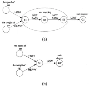
4.2 Transitive fuzzy rule compacting method Considering a simple network constructed as Fig. 4(a),
“the speed of the car” and “the weight of the car” are the input variables, “car stopping” is the hidden variable, and
“safe degree” is the output variable. Respectively, these two rules can be written as:
Rule 1 : IF the speed of the car is HIGH THEN car stopping is NOT EASY.
IF car stopping is NOT EASY, THEN safe degree is LOW.
and the weight of the car is HEAVY, Rule 2:
Obviously, the consequent of Rule 1 is the same as the antecedent of Rule 2, so we can imply the consequent of Rule 2 from the antecedents of Rule 1 directly. That is, these two rules have the transitive relation and can be combined to be:
Rule 1’: IF the speed of the cur is HIGH THEN safe degree is LOW.
and the weight of the cur is HEAVY, Rule 1‘ can then be shown as Fig. 4(b). According to the equation (13) we derived in Section 3, the computational load in Fig. 4(a) is 96 BMO-CLs, and is 63 BMO-CLs after transitive fuzzy rule compacting.
degree the weight of
Fig. 4 (a) Two rules with the transitive situation under the model of KBNNRFS. (b) The result after combining the rules in (a).
In the concept of to combine Rule 1 and consequent of Rule 1 same. Fortunately, they are very similar.
same value througf.
numbers. In this way, domain knowledge computational load decreased, too.
input weight of a weights, the rules transitive relation.
eliminating this G as transitive fuzzy rub:
The transitive described in a two-st1:p (hiddcn G neuron) itt detailed in the following 1) Conditions test
From the examples
During this step, For each G-neuron C relation condition, the computational investigated. When all transitive fuzzy rule performed.
fuzzy theory, it is not always possible Rule 2 under the condition that the and the antecedent of Rule 2 are the nile combination can be applied when This is because we can get almost the defuzzification of similar fuzzy the number of hzzy rules in the fuzzy base can be reduced. Obviously, the during its inference phase can be in Fig. 4, we can find that when the G-neuron is similar to any of its output before and after this G neuron have the We might compact these rules by neuron. Therefore, we term the method fi~zzy rule compacting method can be process for every hidden variable KBNN/TFS. These two steps are
subsections.
compacting method.
we check if the transitive rules exist.
, , three conditions, named transitive hidden variable unused condition and h d decreasing condition, need to be these three conditions are passed, the compacting algorithm can then be
b.) hidden variable U used condition:
hich passes the transitive relation condition will not b used in future, this condition is satisfied. Sometimes. we would like to know the value of the hidden variable di
i
ing inference. In this case, the ruleI f the variable a.) transitive relation
This condition is and after one hidden the transitive relation.
each input connection weight eJ and each
associated with relation condition fcr constraint is met:
Similarity(@. b J ' . vk 7
is bounded between 0 be close to 1 to make similar enough.
The similarity
compacting cannot be applied. The determination of using the hidden variable is made by the user.
condition:
used to determine if the rules before variable (one hidden G-neuron) have For a hidden G-neuron G, , assume I , of G i is associated with a fuzzy output connection 0, of G, is It can be said that the transitive G, is satisfied if the following
. ) 2 6 V j, k (14)
fuiction is defined in Subsection 2 and and 1. The parameter d is defined to sure that the two fuzzy intervals are
c.) computational load decreasing condition:
According to the rule compacting algorithm described in the next subsection, we can preview the compacted structure. The inference computational load of that can be evaluated, too. If the computational load becomes lighter, this condition is satisfied. Before detailing the change of computational load during rule compacting, we need to give the following definitions:
For the ith G-neuron Gi
G-outi : the number of the output connections of G , (the
G-ini : the number of the input connections of Cii (the number of 6 -connections to Gi )
number of SG -connections to Gi )
BS-in . . : input degree of the jth S-neuron which is hehind J'
Gi
FS-inki : input degree af the kth S neuron which is in fkont of G,
In general, the changes of the network structurle after rule compacting on the ith G-neuron can be s m a r i i c e d as:
AN, = -1 (15)
AN, = G-out , * G-out , - G-in , - G-out , (16)
G-w
Aktin-NI,,a, =
+
FS-in, * (G-out, - 1)
k=l G-out,
(BS-inJ, - 1) * (G-in, - 1) - G-ouif, /=I
(17) M g g r - = G -out, * G - in, - G -out, - G -in, ( 1 8) where ANG, ANs , AMin-NITotal and AAggr- NITo,ai are the changes of the numbers of G-neurons, S-neurons, total input connections of S-neurons and total input connections of G- neurons, respectively. According to equation (I 3), which measures the total computational load of the rules, the change of total computational load can then be derived as:
As ATotal-CL < 0, we can make sure that the computational load will decrease after performing rule compacting and the computational load decrleasing condition is satisfied. On the other hand, if ATotal-CL 2 0, it is unnecessary to perform rule compacting.
2) Rule compacting
As the three conditions are passed, rule compacting can be performed by eliminating the hidden variable ( G , ) without changing the logic semantics of rules. Assume FS, indicates the number of S-neurons that are in fi-ont of G, and have a connection with GI . BS, is the number of the S-neurons that are behind of GI and have a connection with G , . The rule compacting algorithm is described in follows.
Rule compacting algorithm:
Step 1) Delete G, and its connected comiections which include some antecedent connections and consequent connections of the rules.
Step 2) Copy ( F S , -1) times the left structure of the rules whose antecedent connections are deleted in Step
1).
Step 3) Copy ( B S I -1) times the left structure of the rules whose consequent connections are deleted in Step Step 4) Combine the S-neurons to build the entire rules and
1).
make sure that no rules are the same.
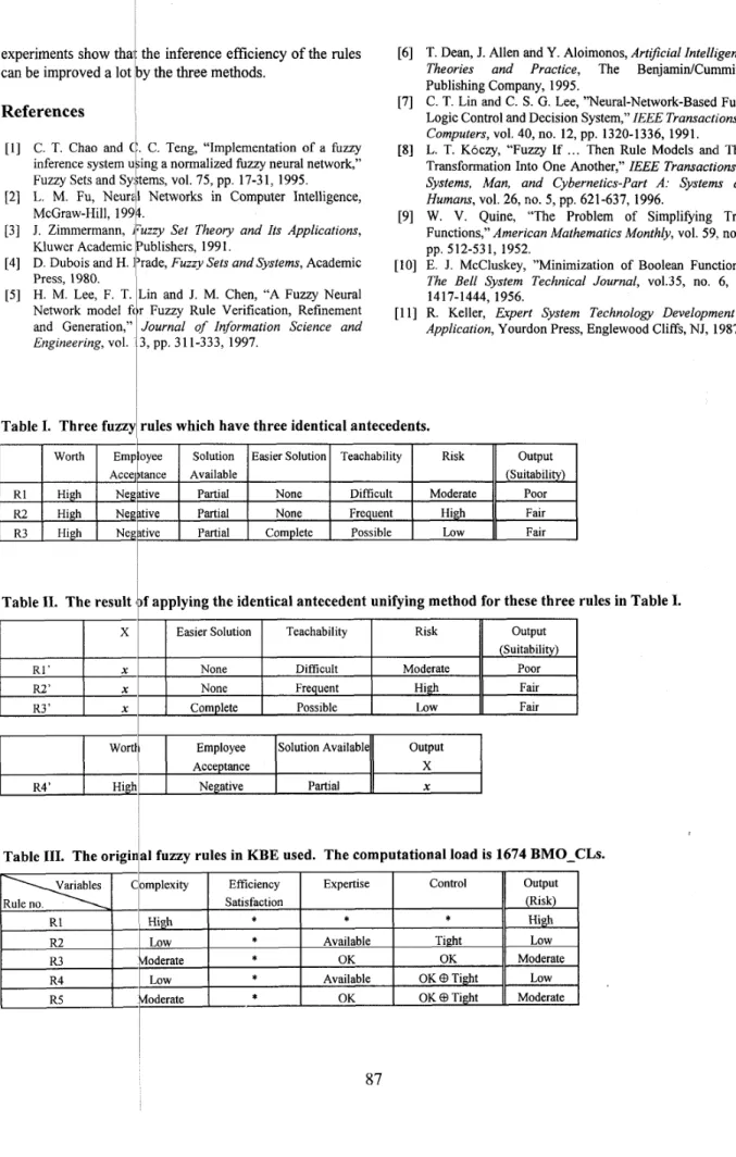
4.3 Identical antecedent unifying method
The third method, called identical antecedent unz&ing method, simplifies the rules that some antecedents in them are the same by replacing the identical antecedents of the rules with a single specific antecedent. A new rule whose antecedents are built as the replaced ones of these simplified rules is inserted to imply the specific antecedents. By this method, many redundant works to measuring the fire degree for the same antecedents of rules are eliminated. Though an additional rule is inserted, the computational load is decreased.
For example, there are three rules listed in Table I.
Obviously, there are three identical antecedents, which are
“WORTH is High”, “EMPLOYEE ACCEPTANCE is Negative” and “SOLUTION A VAILABLE is Partial”, among the three rules. To simply the structure of the rules, we use a specific antecedent, named anonymous antecedent, to replace the three antecedents in each of the rules.
Furthermore, to imply the new anonymous antecedent, a new rule with the three replaced antecedents which are
“WORTH is High”, “EMPLOYEE ACCEPTANCE is Negative” and “SOLUTION AVAILABLE is Partial” is inserted. This anonymous antecedent is defined as “X is x.”
Here, x is a h z z y value (0, 1, 0, 0), and X is an anonymous variable. Table I1 lists the result of applying this structure simplification to these three rules.
According to equation (13), the computational load of the original three rules in Table I is 553 BMO-CLs. After applying the simplification method, the computational load of the four new rules in Table I1 is decreased to 466 BMO-CLs .
5. Experiments
To evaluate the performance of the proposed three efficiency enhancing methods, we implement part of Knowledge Base Evaluator ( D E ) [ 1 11 in DNN/TFS. At first, we use the proposed efficiency validation method to measure the total computational load of these fuzzy rules.
Then, the three efficiency enhancement methods are performed. We use the proposed efficiency validation method again to measure the total computational load of these rules after performing each of the three enhancement methods. Thus, the decreased computational load caused by each enhancement method can be evaluated.
Knowledge Base Evaluator ( D E ) [ 111 is an expert system that evaluates whether the expert system is suitable for a domain or not. Part of its rules is used to implement the structure of neural network in KBNN/TFS. Besides, three other rules which satisfy the three conditions to perform transitive fuzzy rule compacting are included in our experiments. We show all these rules in Table 111. Rules 8, 17 and 18 are the added rules which satisfy the three conditions of performing transitive fmzy rule compacting.
Furthermore, to compare with the outputs of the original rules, the mean square error, denoted E, is defined as:
E = ~ ( D , +%(on -0,)2 +-(D, 1 -0,)~ +-(D~ 1 -0,)2(20)
2 2 2 2
where D = ( D m , D n , D a , D p ) and 6 = ( O m , 0 n , 0 a , 0 , ) are the desired output and network output for some input data, respective. The parameter q is the important factor of mean values m and n. In our experiments, q is set to 3. Table 1V shows the comparison results after performing these three efficiency methods.
6. Conclusion
In this paper, a general efficiency validation method is proposed to evaluate the inference complexity of rules.
According to the definition of the operations on KBNN/TFS and the network structure of rules, the efficiency validation on KBNN/TFS is implemented.
Furthermore, three methods that simplifi the structure of this rule-constructed neural network model are provided to enhance its inference efficiency. The three proposed methods refine the fuzzy rules in the howledge base, and thus increase the speed of inference. It is easy to analysis the result of performing these three efficiency enhancing methods by the proposed validation method. Our
experiments show thai the inference efficiency of the rules can be improved a lot b y the three methods.
[3] J. Zimmermann, Kluwer Academic [4] D. Dubois and H.
Press, 1980.
[5] H. M. Lee, F. T.
Network model and Generation,”
Engineering, vol.
References I I
Fuzzy Set Theovy and Its Applications, Publishers, 1991.
l’rade, Fuzzy Sets and Systems, Academic Lin and J. M. Chen, “A Fuzzy Neural for Fuzzy Rule Verification, Refinement Journal of Information Science and .3, pp. 31 1-333, 1997.
oyee Solution Easier Solution Teachability Risk output
)tame Available (Suitability)
[6] T. Dean, J. Allen and Y. Aloimonos, Artificial Intelligence:
Theories and Practice, The BenjaminlCunimings Publishing Company, 1995.
[7] C. T. Lin and C. S. G. Lee, ”Neural-Network-Based Fuzzy Logic Control and Decision System,” IEEE Transactions on Computers, vol. 40, no. 12, pp. 1320-1336, 1991.
[8] L. T. Koczy, “Fuzzy If ... Then Rule Models andl Their Transformation Into One Another,” ZEEE Transactions on Systems, Man, and Cybernetics-Part A: Systems and Humans, vol. 26, no. 5, pp. 621-637, 1996.
[9] W. V. Quine, “The Problem of Simplifying Truth Functions,” American Mathematics Monthly, vol. 59. no. 8, [ 101 E. J. McCluskey, ”Minimization of Boolean Functions,”
The Bell System Technical Journal, vo1.35, no. 6, pp.
[l I] R. Keller, Expert System Technology Development &
pp. 512-531, 1952.
1417-1444, 1956.
Application, Yourdon Press, Englewood Cliffs, NJ, 1987.
tive tive tive
Table I. Three fuzzy 1 rules which have three identical antecedents.
Partial None Difficult Moderate Poor
Partial None Frequent High Fair
Partial Complete Possible Low Fair
Table 11. The result 1
Table 111. The origin a1 load is 1674 BMO CLs.
Rule no.
R4
R6 R7 R8
Low * Available Loose High
Low 0 Moderate * Unavailable * High
Satisfied Low
* * *
RI 5 RI6
Over 50% Exists Well-Defined Eclectic Moderate
Under 10% Build Fuzzy Eclectic High
Performance
R17 High
RI8 High
Response Time output
Requirement (Efficiency Satisfaction)
Low Satisfied
Moderate Satisfied
Number of Connections
Original 71
(1) 59
(1)+(2) 57
(1)+(2)+(3) 59
Number of Computational load(in Result (MSE)
Rules BMO CLs)
18 1674 0 00000
15 1389 0 00101
14 1356 0 00101
15 1329 0 00101