新興的通用啟發法應用於排程問題

(1)

行政院國家科學委員會專題研究計畫成果報告

新興的通用啟發法應用於排程問題(第 3 年) 研究成果報告(完整版)

計畫類別：個別型

計畫編號： NSC 96-2221-E-011-025-MY3

執行期間： 98 年 08 月 01 日至 99 年 07 月 31 日執行單位：國立臺灣科技大學工業管理系

計畫主持人：廖慶榮

計畫參與人員：碩士班研究生-兼任助理人員：郭紋伶碩士班研究生-兼任助理人員：劉宜婷碩士班研究生-兼任助理人員：王聖瑋博士班研究生-兼任助理人員：鍾翠萍博士班研究生-兼任助理人員：鄒馨慧

處理方式：本計畫涉及專利或其他智慧財產權，2 年後可公開查詢

中華民國 99 年 10 月 26 日

(2)

行政院國家科學委員會補助專題研究計畫 ■ 成果報告

□期中進度報告新興的通用啟發法應用於排程問題

計畫類別：■ 個別型計畫 □ 整合型計畫計畫編號：NSC－96－2221－E－011－025－MY3 執行期間：96 年 8 月 1 日至 99 年 7 月 31 日

計畫主持人：廖慶榮教授

計畫參與人員：鍾翠萍、鄒馨慧、郭紋伶、劉宜婷、王聖瑋

成果報告類型(依經費核定清單規定繳交)：□精簡報告 ■完整報告

本成果報告包括以下應繳交之附件：

□赴國外出差或研習心得報告一份

□赴大陸地區出差或研習心得報告一份

□出席國際學術會議心得報告及發表之論文各一份

□國際合作研究計畫國外研究報告書一份

處理方式：除產學合作研究計畫、提升產業技術及人才培育研究計畫、列管計畫及下列情形者外，得立即公開查詢

□涉及專利或其他智慧財產權，□一年■二年後可公開查詢

執行單位：台灣科技大學工業管理系

中華民國九十九年十月二十五日

(3)

行政院國家科學委員會專題研究計畫成果報告

新興的通用啟發法應用於排程問題

Application of emerging meta-heuristics to scheduling problems

計畫編號：NSC－96－2221－E－011－025－MY3 執行期限：96 年 8 月 1 日至 99 年 7 月 31 日

主持人：廖慶榮教授台灣科技大學工業管理系

計畫參與人員：鍾翠萍台灣科技大學工業管理系博士班鄒馨慧台灣科技大學工業管理系博士班郭紋伶台灣科技大學工業管理系碩士班劉宜婷台灣科技大學工業管理系碩士班王聖瑋台灣科技大學工業管理系碩士班

中文摘要

蟻群最佳化（Ant Colony Optimization；ACO）與粒子群演算法（Particle Swarm Optimization；PSO）為具有潛力的兩種新興通用啟發法，透過轉換，可以應用於各種問題。在本研究中，我們依序探討在供應鏈、越庫作業與混合流程型工廠下，三種不同生產環境的排程問題，透過引入派工法則以及混合其它通用啟發法的方式，提出更有效的 ACO 與 PSO，希望未來有機會能應用在實務問題上。研究主要區分為以下三個部分：

Part I: 應用蟻群最佳化協調兩階段生產系統之整備時間

在第一年度中，我們應用ACO 於排程問題。ACO 是一個啟發自螞蟻群體合作行為

之新興共通啟發式演算法。目前蟻群最佳化已廣泛應用於各種最佳化組合問題上，如銷售員問題（Traveling Salesman Problems；TSP）、二次指派問題（Quadratic Assignment Problems；QAP）及車輛派遣問題（Vehicle Routing Problems；VRP），但蟻群最佳化應用於排程問題之研究上仍相當稀少。因此，本研究將應用蟻群最佳化於協調兩階段供應鍊之時間成本問題。

本研究考量協調兩階段供應鍊之時間成本問題。此問題是由一個廚房家具工廠其製造鍊之實際應用延伸而來。工廠包含兩連續加工階段，即切割與塗漆作業。在不同階段中，所有屬性皆相同之物品組成一批量。同一階段內，當一組新批量的屬性類別和前一批量的屬性類別不同時，即產生整備成本，此成本與批量先後次序無關。本研究之目標為決定所有批量之順序，以最小化總整備時間成本。本研究中，我們首度提出一派工法則，可相當有效率地產生比基因演算法（Genetic Algorithm；GA）更好的解。此演算法

結合派工法則與產生初始解之方法，發展一 ACO 以更進一步改善此解，並在極短的運

算時間下，得到顯著優於其他之共通啟發式演算法，實驗結果顯示我們提出之 ACO 演

算法有很好的求解效果。

Part II: 粒子群演算法應用於越庫作業系統之時窗車輛指派問題

越庫作業被認為是一個在供應鏈管理中能夠有效控制存貨流動的方法，在第二年度中，我們將探討粒子群最佳化演算法（PSO）應用於越庫作業系統之時窗車輛指派問題。

在這個模型之中，每台車輛都有時間窗的限制，且車輛數超過現有的碼頭數。問題主要

(4)

統的總容量限制。在考慮卡車停靠在碼頭的總運營成本和對未完成發貨的處罰成本最小

化下，來求解卡車的最佳指派。我們提出兩個啟發法求解此問題，並配合PSO。實驗結

果證明，該啟發式演算法比現有的禁忌搜索（TS）法在計算時間與結果上，表現均為優

良，而PSO 也可在短的時間內得到近似最佳解。

Part III: 應用離散粒子群最佳化演算法與瓶頸法求解混合流程型工廠排程問題

在許多產業中，混合流程型工廠（HFS）是一個普遍的生產環境，例如玻璃業、鋼鐵業、造紙業與紡織業等。因此，我們發展一個粒子群最佳化演算法（PSO）來求解混合流程型工廠排程問題，目標設定為最小總完工時間。此研究的主要貢獻分為兩方面：

(1)在瓶頸階段時，應用離散型 PSO 與瓶頸法混合來強化搜尋能力，(2)引入模擬退火法

來跳脫局部最佳解。另外，加入一個重新啟動的過程，避免過早收斂。經過實驗於Carlier

與 Néron 提出來的標竿題庫上，我們所提出的 PSO 優於目前所有求解混合流程型工廠

排程問題的演算法。

關鍵詞：蟻群最佳化演算法、粒子群演算法、排程、啟發式、供應鍊、派工法則、越庫作業、卡車指派問題、混合流程型工廠、總完工時間、模擬退火法、瓶頸法。

Abstract

Ant Colony Optimization (ACO) and Particle Swarm Optimization (PSO) are two potential emerging meta-heuristics. By transforming, they can be applied to varied problems.

In this research, we consider scheduling problems in three different production environments:

supply chain, truck dock assignment and hybrid flow shop. In order to solve these problems, we propose efficient ACO and PSO by means of incorporating dispatching rules and mixing other meta-heuristics. The research includes the following three parts:

Part I: An Ant Colony Optimization Algorithm for Setup Coordination in a Two-Stage Production System.

We apply ACO to scheduling problem in the first year. ACO is a novel metaheuristic inspired by the cooperation behavior of ants. Nowadays, ACO has extensively applied to a large number of combinatorial optimization problems, such as traveling salesman problems (TSP), quadratic assignment problems (QAP), and vehicle routing problems (VRP), but the applications of ACO to scheduling problems are extremely few. Hence, this research will apply ACO to the coordination of setup costs in a two-stage supply chain.

This problem is derived from a furniture plant, where there are two consecutive departments, including cutting department and painting department. In different departments, items are grouped according to different attributes. A sequence-dependent setup cost is required in a stage when the new batch has a different level of attribute from the previous one.

The objective is to minimize the total setup cost. In this paper, we first propose a simple dispatching rule, which can yield a solution better than the existing genetic algorithm while using much less computation time. Incorporating the dispatching rule as the initial solution method, an ACO algorithm is developed to further improve the solution. Computational experiments show that the proposed ACO algorithm is quite effective in finding the near-optimal solution.

Part II: An approach using particle swarm optimization to solve truck dock assignment problem in cross docking systems with operational time constraint

(5)

In the second year, we consider a truck dock assignment problem with an operational time constraint in a crossdock where the number of trucks exceeds the number of docks available. The objective of the problem is to find an optimal truck dock assignment to minimize the sum of the total dock operational cost and the penalty cost for all the unfulfilled shipments. The problem feasibility is affected by three factors: the arrival and departure time windows of each truck, the operational time for the cargo shipments among the docks, and the total capacity available to the crossdock. We propose fast and effective heuristics for determining very good solutions for the problem. To further improve the solution, a Particle Swarm Optimization (PSO) algorithm combined with the heuristics is also developed.

Computational experiments show that the heuristics themselves perform better than an existing tabu search (TS) algorithm in terms of computation time and solution quality.

Considering only the metaheuristic itself, the PSO algorithm also outperforms the TS algorithm when both employing the heuristics.

Part III: An approach using particle swarm optimization and bottleneck heuristic to solve hybrid flow shop scheduling problem

The hybrid flow shop (HFS) is a common manufacturing environment in many industries, such as the glass, steel, paper and textile industries. In this research, we present a particle swarm optimization (PSO) algorithm for the HFS scheduling problem with minimum makespan objective. The main contribution of this paper is to develop a new approach hybridizing PSO with bottleneck heuristic to fully exploit the bottleneck stage, and with simulated annealing to help escape from local optima. A restart procedure is also employed to avoid premature convergence. The proposed PSO algorithm is tested on the benchmark problems provide by Carlier and Néron. Experiment results show that the proposed algorithm outperform all the compared algorithms in solving the HFS problem.

Keywords: Ant colony optimization; Particle swarm optimization; Simulated annealing;

Scheduling; Supply chain; Crossdock; Hybrid flow shop

(6)

Part I. An ant colony optimization algorithm for setup coordination in a two- stage production system.

1. Introduction

This paper deals with a real problem of a two-stage production system proposed by Agnetis et al. [1]. The problem arises from the manufacturing of a kitchen furniture plant, where there are two consecutive departments including cutting and painting departments. In different departments, items are grouped according to different attributes. In the cutting department, items are grouped according to their shape, and in the subsequent painting department, they are grouped according to their color.

In this production environment, each attribute has many different levels. A batch consists of all the items having the same levels for all attributes. A setup occurs when the new batch has a level of an attribute different from the previous batch. Since no buffer is available between two consecutive departments, these departments have to follow the same batch sequence. Hence, we need only to determine a permutation of batches.

Agnetis et al. [1] considered the problem with two objectives. One is minimizing the total number of setups (MINSUM) in the two departments, and the other is minimizing the maximum number of setups (MINMAX) in either department. It was assumed that all the setup times are equal and sequence independent, i.e., unitary setup time. This implies that in the painting department the setup changed from blue to white has the same time as that changed from white to blue. Each of the two objectives has been proved to be NP-hard by Agnetis et al. [1].

Several heuristics have been proposed for the problem. For the MINSUM objective, Agnetis et al. [1] and Meloni [2] proposed a constructive heuristic and a metaheuristic for the problem, respectively. Both solution approaches perform satisfactorily on a set of real cases and a large sample of experimental data. Considering both MINSUM and MINMAX simultaneously as a multi-objective problem, most studies applied metaheuristics to find a good approximation of the Pareto-optimal front. Mansouri [3] proposed a multi-objective genetic algorithm (MOGA), and shortly after Mansouri [4] presented a better multi-objective simulated annealing (MOSA).

Recently, Detti et al. [5] developed a graph-based ILS algorithm in which two greedy heuristics are used to obtain the initial solution. The computational results show that the ILS algorithm combining with the initial solution can obtain the effectiveness with respect to solution quality and computation time.

A unitary setup time is assumed in all the papers discussed above. However, an explicit consideration of sequence-dependent setup time is usually required in many practical manufacturing environments, including the furniture manufacturing. As an illustration in the painting department, the setup time changed from blue to white is usually different from that changed from white to blue. Naso et al. [6] considered the problem with sequence-dependent setup times and presented a genetic algorithm for the MINSUM objective. In this paper, we address the same problem as Naso et al. [6] and propose an Ant Colony Optimization (ACO) approach for the problem.

2. Problem formulation

In this section, we give a formal description of the problem. The following notation is used throughout the paper:

Q a sequence of the batches D stage j j j, =1, 2

|D | number of stages

(7)

B set of batches

| |B number of batches

A j set of all possible levels of attribute j

|A _j| number of levels of attribute j b batch i i i, =1, 2, ,| |⋅⋅⋅ B

j( )i

a b level of attribute j for bⁱ

[ ]k

b batch scheduled in the kth position, k=1, 2,⋅⋅⋅| |B ( )_i

f b flexibility index of b (defined as the number of batches with a level of attribute _i same as b ) _i

[ ] [ ]¹

( ), ( )

j k j k

a b a b

s ₊ setup time between batches k and k+1 in stage D _j U set of unscheduled batches

Z j total setup time in stage D in a sequence _j ( )

Z σ total setup time of partial sequence σ ( , )

Z σ i total setup time after batch b is appended to partial sequence _i σ

The two-stage coordination problem with sequence-dependent setup times consists in scheduling a set of batches B on the two stages D and ₁ D . Because no buffer is available ₂ between the two consecutive stages, the sequence Q in which each stage processes all batches is identical on the two stages. Hence, we need only to determine a permutation of batches for the problem.

Each batch is characterized by two attributes a and ₁ a . Let ₂ A and ₁ A denote the sets of ₂ all possible levels of a and ₁ a , respectively. Let ₂ b_{[ ]}_k denote the batch scheduled in the kth position of a sequence. For two consecutive batches b_{[ ]}_k and b_{[ ]}_k₊₁ , a setup time

[ ] [ ]¹

( ), ( )

j k j k

a b a b

s + is

required in stage D if _j a b_j( _{[ ]}_k )≠a b_j( _{[ ]}_k₊₁) . Following [6], the sequence-dependent setup time for each couple of different levels of attribute a is generated from a discrete uniform distribution _j

(1,| |)_j

U A . Thus, there exists a square setup time matrix for each of the two attributes.

For a given sequence Q , we can calculate the setup times incurred in the two stages, denoted by Z Q and ₁( ) Z Q , as follows: ₂( )

[ ] [ ]

1 1 1

2 2 1

| | 1

1 ( ), ( )

1

| | 1

2 ( ), ( )

1

( )

k k

B

a b a b

k B

a b a b

k

Z Q s

+

−

=

−

=

∑

The objective of the problem can be expressed as

Min Z =Z Q₁( )+Z Q₂( )

Actually, the problem is a Traveling Salesman Problem (TSP), a well known optimization problem.

Since the matrixes of setup times are not symmetric, it is an asymmetric TSP.

3. Proposed Algorithms

In this section, we first propose a dispatching rule for the problem. Incorporating the dispatching rule, an ACO algorithm is then developed to obtain a near-optimal solution.

(8)

In this section we develop a dispatching rule for the two-stage production system with sequence-dependent setup times. The presented dispatching rule can not only be used as a heuristic for the problem, but also be used as the initial solution method and the heuristic desirability in the ACO algorithm.

The dispatching rule was inspired by the least flexibility first heuristic (LFFH) (Liao et al. [7]).

In addition to the flexibility index, we need to consider the magnitude of the setup times. The dispatching rule combines the flexibility index and the setup times into a single index. According to the rule, the batches are assigned in non-increasing order of the ranking index given by

( )

¹

exp ( )

( , ) ( )

i i

I f b

Z i Z

λ σ σ

= −

−

where ( )f b is the flexibility index of batch i , _i Z( , )σ i −Z( )σ is the advancement of total setup time when batch i is appended to partial sequence σ , and λ is the flexibility-related scaling parameter. Hereafter, the dispatching rule will be referred to as the Least Flexibility with Setups (LFS) rule.

3.2 The proposed ACO algorithm

We now address the details of each step of the proposed ACO algorithm.

Step 1. Initialize pheromone

Most ACO algorithms set τ₀ =1/(n Z× ), where Z is the objective value of a solution obtained either randomly or through some simple heuristic. However, our experimental analyses show that this setting of τ₀ results in premature convergence for the considered problem (see Section 4). To avoid premature convergence, we remove n from the denominator and use the LFS rule to obtain the Z value, i.e., τ₀ =1/(Z_LFS).

Step 2. Main loop

In the main loop, we randomly put m ants at m start positions. Each of the m ants constructs a sequence of | |B batches. The loop is executed for a maximum of 1100 consecutive iterations (MaxIter 1100= ).

Step 2.1 Construct a feasible solution by each ant

A set of artificial ants is initially created. Each ant starts with an empty sequence and then successively appends an unscheduled batch to the partial sequence until a feasible schedule is constructed. The ant chooses an unscheduled batch j among the set of unscheduled batches U by applying the following probabilistic formulation:

{ }

⁰

arg max [ ( , )] [ ( , ) ] if

otherwise

u U t i u i u q q

j S

τ η β

∈

⎧ ⋅ ≤

= ⎨⎪

⎪⎩

where ( , )τ_t i u is the pheromone trail associated with the movement from batch i to batch u at time t , ( , )η i u is the heuristic desirability of moving batch i to batch u, and β is the parameter which determines the relative importance of the heuristic information. In our ACO algorithm, we use the LFS rule as the heuristic desirability. q is a random number uniformly distributed in [0,1] , and q is a parameter ₀ (0≤q₀ ≤ which determines the relative importance 1) of exploitation versus exploration. If q≤ , the unscheduled batch j with maximum value is q₀ selected to move from batch i (exploitation), otherwise a batch is chosen according to a random variable S (biased exploration). S is selected according to a probability distribution given by:

[ ( , )] [ ( , )]

( , )

[ ( , )] [ ( , )]

t t u U

i u i u p i j

i u i u

β β

τ η

∈

= ⋅

∑

⋅

(9)

Step 2.2 Local update of pheromone trail

To avoid premature convergence, a local trail update is performed. The update reduces the amount of pheromone for the newly added batch so as to discourage the following ants from choosing the same batch. This is achieved by the following local updating rule:

( , ) (1 ) ( , ) 0

t i j t i j

τ = −ρ τ +ρτ where (0ρ < ≤ . ρ 1)

Step 2.3 Local search

The local search used in our ACO algorithm is the Random Job Insertion Local Search (RJILS) proposed by Gajpal and Rajendran [8]. The RJILS rule can be described as follows:

1. Set initial sequence S . _k

2. Randomly choose a batch from B and insert it in all possible positions of S . Choose the best _k sequence S with minimum total setup time. Update _c S by _k S if the latter is better and _c retain S otherwise. _k

3. Randomly choose another batch from B and repeat Step 2 until all batches in B are selected once and only once.

In order to evaluate the performance of RJILS in our ACO, computational experiments will be conducted to compare with two popular local searches: 2-OPT (Nillson [9]) and SWAP (Liao and Cheng [10]) in Section 4.

Step 2.4 Global update of pheromone trail

The global updating rule is applied after each ant has completed a feasible solution and the local search has been implemented. Following the rule, the pheromone trail is added to the path of the incumbent global best solution. If the path of batch i to batch j belongs to one part of incumbent global best solution, then

1( , ) (1 ) ( , ) ( , )

t i j i j t i j

τ₊ = −α τ⋅ + Δα τ

where α (0< ≤ is a parameter representing the evaporation of pheromone. The amount α 1) ( , )

t i j

τ

Δ equals 1/ Z , where ^* Z is objective value of the global best solution. However, our ^* experimental analyses show that this setting of Δτ_t( , )i j result in premature convergence for our problem. To improve this situation, we try to add more pheromone density in the path of global best solution leaving more effect of elitist strategy. So the modified global update function becomes

1( , ) (1 ) ( , ) ( , )

t i j i j t i j

τ ₊ = −α τ⋅ + Δτ

where Δτ_t( , )i j =R Z/ ^*. The amount R is parameter which increases more amount of pheromone density. The resulting performance will be shown in Section 4. Moreover, to avoid the solution falling into a local optimum that results from the pheromone evaporating to zero, we introduce a lower bound to the pheromone trail value by letting τ_t( , ) (1/ 5)i j = τ₀ (Stützle and Hoos [11]).

4. Computational results

To verify the performance of the LFS rule and the ACO algorithm, two sets of computational experiments were conducted. The first one is for the parameter settings, including τ₀, global updating rule, and local search. The second one is to compare the proposed algorithm with the genetic algorithm of Naso et al. [6], denoted by GA hereafter, and two other ACO algorithms. The test problem instances were generated using the same scheme as Naso et al. [6].

Three different sizes of attributes were tested (i.e., |A₁| |= A₂| 10, 20,30= ), and each size was assigned a density from 0.1 to 0.4. The setup times for each couple of different levels of attributes were generated from a discrete uniform distribution ^U

(

^1,|^A ^|

)

^{, 1, 2}^j⁼ (Naso et al. [6]). This

(10)

results in a total of 12 problem instances. The density is defined as the number of batches with respect to the total number of possible combinations of attributes, i.e., density | |= B

∏

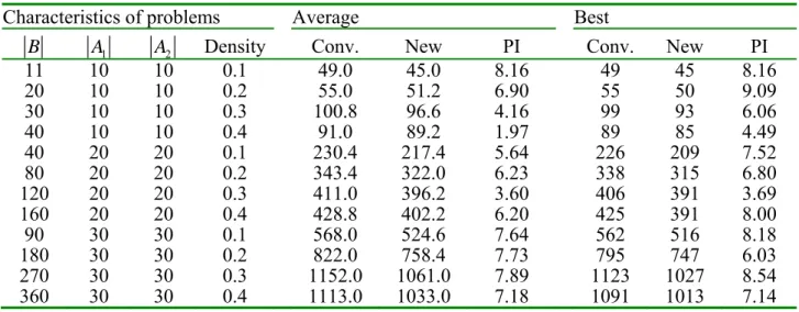
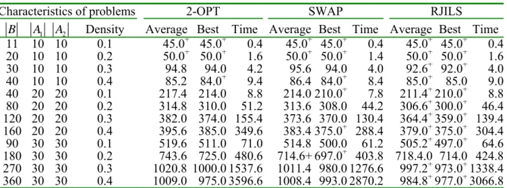
^{| |}^D_j₌₁|A_j| (Agnetis et al. [1]). To determine the best values of ACO parameters, a series of pilot experiments was conducted. The best values for our problem are as follows: Itemax=1100, m=8, ρ=0.1, α =0.1, 2β = , λ=0.02, q₀ =0.9, R=25 In all the experiments, each of the compared algorithms was run five times for each instance and their average was recorded as the solution of the algorithm.

In the first set of experiments, we evaluate the impact of the new τ₀ and the global updating rule in the ACO algorithm. To make a clear comparison, we temporarily remove the local search from the algorithm. Tables 1 and 2 give the computational results, which indicate that the new τ₀ and the global update rule can improve the solutions with average improvements of 6.04% and 6.11%, respectively. To evaluate the performance of RJILS, comparisons were conducted with 2-OPT and SWAP local searches. The termination condition was set by letting MaxIter=1100. Table 3 gives the computational results, which demonstrate that in general RJILS is superior to the other two local search methods.

Table 1. The comparison of conventional and new τ₀

Characteristics of problems Average Best

B A₁ A₂ Density Conv. New PI Conv. New PI

11 10 10 0.1 46.8 45.8 2.13 45 45 0.00

20 10 10 0.2 54.6 50.8 6.95 50 50 0.00

30 10 10 0.3 101.2 96.6 4.54 98 93 5.10

40 10 10 0.4 97.8 88.8 9.20 91 85 6.59

40 20 20 0.1 225.2 223.6 0.70 219 221 −0.90

80 20 20 0.2 343.0 327.0 4.66 333 315 5.40

120 20 20 0.3 442.2 394.2 10.85 420 385 8.33

160 20 20 0.4 431.4 401.2 7.00 417 400 4.07

90 30 30 0.1 572.2 532.0 7.02 554 520 6.13

180 30 30 0.2 804.0 750.0 6.71 769 727 5.46

270 30 30 0.3 1132.0 1061.0 6.27 1115 1027 7.89

360 30 30 0.4 1104.6 1033.0 6.48 1054 1013 3.88

PI: percentage improvement

Table 2. The comparison of conventional and new global update rule

Characteristics of problems Average Best

B A₁ A₂ Density Conv. New PI Conv. New PI

11 10 10 0.1 49.0 45.0 8.16 49 45 8.16

20 10 10 0.2 55.0 51.2 6.90 55 50 9.09

30 10 10 0.3 100.8 96.6 4.16 99 93 6.06

40 10 10 0.4 91.0 89.2 1.97 89 85 4.49

40 20 20 0.1 230.4 217.4 5.64 226 209 7.52

80 20 20 0.2 343.4 322.0 6.23 338 315 6.80

120 20 20 0.3 411.0 396.2 3.60 406 391 3.69

160 20 20 0.4 428.8 402.2 6.20 425 391 8.00

90 30 30 0.1 568.0 524.6 7.64 562 516 8.18

180 30 30 0.2 822.0 758.4 7.73 795 747 6.03

270 30 30 0.3 1152.0 1061.0 7.89 1123 1027 8.54

360 30 30 0.4 1113.0 1033.0 7.18 1091 1013 7.14

PI: percentage improvement

(11)

Table 3. Comparison of some local searches

Characteristics of problems 2-OPT SWAP RJILS

B A₁ A₂ Density Average Best Time Average Best Time Average Best Time 11 10 10 0.1 45.0⁺ 45.0⁺ 0.4 45.0⁺ 45.0⁺ 0.4 45.0⁺ 45.0⁺ 0.4 20 10 10 0.2 50.0⁺ 50.0⁺ 1.6 50.0⁺ 50.0⁺ 1.4 50.0⁺ 50.0⁺ 1.6 30 10 10 0.3 94.8 94.0 4.2 95.6 94.0 4.0 92.6⁺ 92.0⁺ 4.0 40 10 10 0.4 85.2 84.0⁺ 9.4 86.4 84.0⁺ 8.4 85.0⁺ 85.0 9.0 40 20 20 0.1 217.4 214.0 8.8 214.0 210.0⁺ 7.8 211.4⁺210.0⁺ 8.8 80 20 20 0.2 314.8 310.0 51.2 313.6 308.0 44.2 306.6⁺300.0⁺ 46.4 120 20 20 0.3 382.0 374.0 155.4 373.6 370.0 130.4 364.4⁺359.0⁺ 139.4 160 20 20 0.4 395.6 385.0 349.6 383.4 375.0⁺ 288.4 379.0⁺375.0⁺ 304.4 90 30 30 0.1 519.6 511.0 71.0 514.8 500.0 61.2 505.2⁺497.0⁺ 64.6 180 30 30 0.2 743.6 725.0 480.6 714.6+ 697.0⁺ 403.8 718.4.0 714.0 424.8 270 30 30 0.3 1020.8 1000.0 1537.6 1011.4 980.0 1276.6 997.2⁺973.0⁺1338.4 360 30 30 0.4 1009.0 975.0 3596.6 1008.4 993.0 2870.2 984.8⁺977.0⁺3066.8 +The proposed approach is best

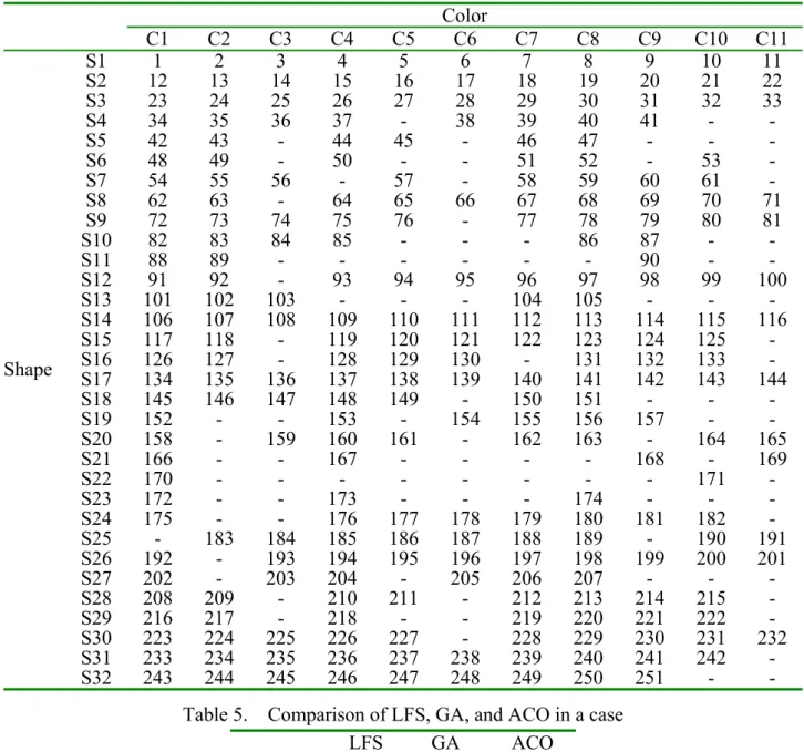
In the second set of experiments, we first tested a case provided by Naso et al. [6]. The instance describes a weekly product demand based on the actual customer orders in a furniture plant. Table 4 shows a weekly production plan consisting of 251 production batches with 32 cutting classes and 11 color classes. The setup times for each couple of different levels of attributes are random numbers selected in the range [1,| 32 |] for the cutting department and [1,|11|] for the painting department. There are 251! possible sequences in the instance. We compare the solutions obtained by GA, LFS, and ACO. The results are summarized in Table 5, which shows that for this real case the LFS rule presents a better performance than GA while using much less computation time. The ACO algorithm can further improve the solutions from LFS with more computational requirements.

To further evaluate the performance of the proposed algorithm, we established a comparison among LFS, GA, GA/LFS (using LFS as one seed), and ACO on a large sample of experimental data. For a fair comparison, all the four algorithms were coded in C++ and run on the same PC environment. The maximum iteration of ACO was set as 500 while the maximum iterations of GA and GA/LFS were set flexible to make the three algorithms have roughly the same computation time. From Table 6, it can be observed that the LFS rule yields results significantly better than GA while using much less computation time (except for some small problems). Besides, the GA/LFS outperforms GA for all the instances, which indicates the advantage of using LFS in GA. The ACO algorithm can further improve the solution from the LFS dispatching rule and it performs best for all the instances.

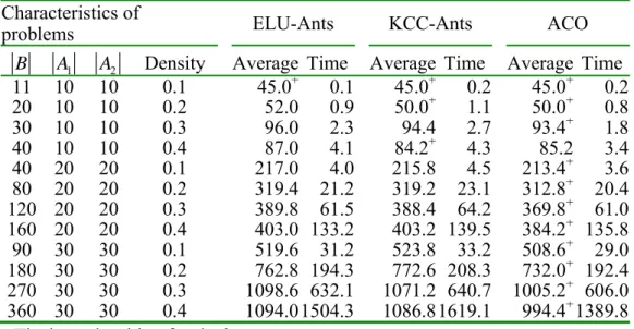
Finally, we made a comparison of our ACO with two new ACO algorithms of Hossein and Nima [12], i.e., KCC-Ants and ELU-Ants, that were designed for solving the traveling salesman problem (TSP). The two ACO algorithms contain new and reasonable local updating rules that make them more efficient in solving TSP. As mentioned earlier, our problem is equivalent to an asymmetric TSP problem, so KCC-Ants and ELU-Ants can be used to solve our problem. To make a fair comparison, we use the LFS rule and the new local search in both KCC-Ants and ELU-Ants.

Both KCC-Ants and ELU-Ants were run 700 iterations and ACO was run 500 iterations so as to achieve roughly the same computational time. From Table 7, it can be observed that KCC-Ants outperforms ELU-Ants. ACO and KCC-Ants have similar performance for small problems, but ACO is always superior to KCC-Ants when the number of batches exceeds 40 batches.

(12)

Table 4. A real case with 251 production batches Color

C1 C2 C3 C4 C5 C6 C7 C8 C9 C10 C11

Shape

S1 1 2 3 4 5 6 7 8 9 10 11

S2 12 13 14 15 16 17 18 19 20 21 22

S3 23 24 25 26 27 28 29 30 31 32 33

S4 34 35 36 37 - 38 39 40 41 - -

S5 42 43 - 44 45 - 46 47 - - -

S6 48 49 - 50 - - 51 52 - 53 -

S7 54 55 56 - 57 - 58 59 60 61 -

S8 62 63 - 64 65 66 67 68 69 70 71

S9 72 73 74 75 76 - 77 78 79 80 81

S10 82 83 84 85 - - - 86 87 - -

S11 88 89 - - - 90 - -

S12 91 92 - 93 94 95 96 97 98 99 100

S13 101 102 103 - - - 104 105 - - -

S14 106 107 108 109 110 111 112 113 114 115 116 S15 117 118 - 119 120 121 122 123 124 125 - S16 126 127 - 128 129 130 - 131 132 133 - S17 134 135 136 137 138 139 140 141 142 143 144 S18 145 146 147 148 149 - 150 151 - - -

S19 152 - - 153 - 154 155 156 157 - -

S20 158 - 159 160 161 - 162 163 - 164 165

S21 166 - - 167 - - - - 168 - 169

S22 170 - - - 171 -

S23 172 - - 173 - - - 174 - - -

S24 175 - - 176 177 178 179 180 181 182 - S25 - 183 184 185 186 187 188 189 - 190 191 S26 192 - 193 194 195 196 197 198 199 200 201

S27 202 - 203 204 - 205 206 207 - - -

S28 208 209 - 210 211 - 212 213 214 215 - S29 216 217 - 218 - - 219 220 221 222 - S30 223 224 225 226 227 - 228 229 230 231 232 S31 233 234 235 236 237 238 239 240 241 242 - S32 243 244 245 246 247 248 249 250 251 - -

Table 5. Comparison of LFS, GA, and ACO in a case

LFS GA ACO

Solution 619.2 1151.8 510.8

Time 0.07 643.6 534.8

Table 6. Comparison of LFS, GA, GA/LFS, ACO

Characteristics of problems LFS GA GA/LFS ACO

B A₁ A₂ Density Average Time Average Time Average Time Average Time 11 10 10 0.1 64.0 0.000 48.8 2.8 48.8 2.7 45.0⁺ 0.2 20 10 10 0.2 78.6 0.000 65.2 4.6 55.4 4.5 50.0⁺ 0.8 30 10 10 0.3 123.6 0.003 115.8 7.3 106.8 7.3 93.4⁺ 1.8 40 10 10 0.4 114.8 0.000 129.6 10.7 97.4 10.5 85.2⁺ 3.4 40 20 20 0.1 278.6 0.000 310.8 10.6 243.8 10.5 213.4⁺ 3.6 80 20 20 0.2 408.2 0.003 491.4 30.9 367.2 30.9 312.8⁺ 20.4 120 20 20 0.3 511.8 0.006 749.6 62.7 458.8 62.0 369.8⁺ 61.0 160 20 20 0.4 514.8 0.024 81 132 465 132 384.2⁺ 135.8 90 30 30 0.1 665.8 0.006 878.6 37.1 579.0 36.4 508.6⁺ 29.0 180 30 30 0.2 920.8 0.031 1465.0 342.6 848.0 344.2 732.0⁺ 192.4 270 30 30 0.3 1240.4 0.087 2219.6 727.4 1167.0 727.3 1005.2⁺ 606.0 360 30 30 0.4 1201.6 0.190 2653.2 1551.4 1089.2 1531.7 994.4⁺1389.8 +The proposed algorithm is best

(13)

Table 7. Comparison of ELU-Ants, KCC-Ants, and ACO Characteristics of

problems ELU-Ants KCC-Ants ACO

B A₁ A₂ Density Average Time Average Time Average Time 11 10 10 0.1 45.0⁺ 0.1 45.0⁺ 0.2 45.0⁺ 0.2 20 10 10 0.2 52.0 0.9 50.0⁺ 1.1 50.0⁺ 0.8

30 10 10 0.3 96.0 2.3 94.4 2.7 93.4⁺ 1.8

40 10 10 0.4 87.0 4.1 84.2⁺ 4.3 85.2 3.4

40 20 20 0.1 217.0 4.0 215.8 4.5 213.4⁺ 3.6 80 20 20 0.2 319.4 21.2 319.2 23.1 312.8⁺ 20.4 120 20 20 0.3 389.8 61.5 388.4 64.2 369.8⁺ 61.0 160 20 20 0.4 403.0 133.2 403.2 139.5 384.2⁺ 135.8

90 30 30 0.1 519.6 31.2 523.8 33.2 508.6⁺ 29.0 180 30 30 0.2 762.8 194.3 772.6 208.3 732.0⁺ 192.4 270 30 30 0.3 1098.6 632.1 1071.2 640.7 1005.2⁺ 606.0 360 30 30 0.4 1094.01504.3 1086.81619.1 994.4⁺ 1389.8 +The best algorithm for the instance

5. Conclusions and future research

This paper has investigated the setup coordination problem in a two-stage production system where the setup times are sequence independent. The objective is to minimize the total setup time in the two stages. First, we have proposed an LFS dispatching rule, which combines the flexibility index and the setup times into a single index. Then, an ACO algorithm is developed to obtain a near-optimal solution. ACO is chosen as the solution approach because the problem is equivalent to an asymmetric Traveling Salesman Problem (TSP). The developed ACO algorithm has several features that make it effective for the problem.

To evaluate the LFS rule and the ACO algorithm, they have been compared with an existing genetic algorithm and two new ACO algorithms for solving TSP. Computational results show that the LFS rule is quite useful and the ACO algorithm performs significantly better than the genetic algorithm and the two ACO algorithms.

References

[1] Agnetis A, Detti P, Meloni C, Pacciarelli D. Set-up coordination between two stages of a supply chain. Annals of Operation Research 2001; 107: 15–32.

[2] Meloni C. An Evolutionary algorithm for the sequence coordination in furniture production.

Lecture Notes of Computer Science 2001; 2264: 91–106.

[3] Mansouri S A. Coordination of set-ups between two stages of a supply chain using multi-objective genetic algorithms. International Journal of Production Research 2005; 43:

3163–3180.

[4] Mansouri S A. A simulated annealing approach to a bi-criteria sequencing problem in a two-stage supply chain. Computers and Industrial Engineering 2006; 50: 105–119.

[5] Detti P, Meloni C, Pranzo M, Minimizing and balancing setups in a serial production system.

International Journal of Production Research 2007; 45: 5769–5788.

[6] Naso D, Turchiano B, Meloni C. Single and multi-objective evolutionary algorithms for the coordination of serial manufacturing operations. Journal of Intelligent Manufacturing 2006;

17: 251–270.

(14)

[7] Liao C J, Shyu C C, Tseng C T. A least flexibility first heuristic to coordinate setups in a two- or three-stage supply chain. International Journal of Production Economics 2009; 117:

127–135.

[8] Gajpal Y, Rajendran C, Ziegler H. An ant colony algorithm for scheduling in flowshops with sequence-dependent setup times of jobs. The International Journal of Advanced Manufacturing Technology 2006; 30: 416–424.

[9] Nilsson C. Heuristics for the traveling salesman problem. Tech. Repot, Linkoping University, Sweden. http://www.ida.liu.se/TDDB19/reports_2003

[10] Liao C J, Cheng C C. A variable neighborhood search for minimizing single machine weighted earliness and tardiness with common due date. Computers and Industrial Engineering 2007; 52: 404–413.

[11] Stützle T, Hoos H H. Max-min ant system. Future Generation computer system 2000; 16:

889–914.

[12] Hossein M N, Nima T. New robust and efficient ant colony algorithms: Using new interpretation of local updating process. Expert Systems with Applications 2009; 36: 481–488.

[13] Bauer A, Bullnheimer B, Hartl R F, Strauss C. An ant colony optimization approach for the single machine total tardiness problem. Proceedings of the 1999 Congress on Evolutionary Computation. New York: IEEE Press; 1445–1450.

[14] Bullnheimer B, Hartl R F, Strauss C. An improved ant system algorithm for the vehicle routing problem. Annals of Operations Research 1999; 89: 319–28.

[15] Cheng T C E, Lazarev A A, Gafarov E R. A hybrid algorithm for the single-machine total tardiness problem. Computers and Operations Research 2009; 36: 308–315.

[16] Dorigo M, Caro G Di. The Ant Colony Optimization meta-heuristic. In Corne D, Dorigo M, Glover F, editors, New Ideas in Optimization, pages 11–32. McGraw-Hill 1999.

[17] Dorigo M, Gambardella L M. Ant colony system: a cooperative learning approach to the traveling salesman problem. IEEE Transactions on Evolutionary Computation 1997; 1: 53–66.

[18] Gambardella L M, Taillard E D, Dorigo M. Ant colonies for the quadratic assignment problem.

Journal of Operational Research Society 1999; 50: 167–176.

[19] Hamed Q S, Babak A, Amirhosein M K. Website structure improvement: Quadratic assignment problem approach and ant colony meta-heuristic technique. Applied Mathematics and Computation 2008; 195: 285–298.

[20] Lawler E L, Lenstra J K, Rinnooy Kan A H G, Shmoys D B. The Traveling Saleman Problem.

Wiley 1985.

[21] Naimi H M, Taherinead N. New robust and efficient ant colony algorithms: Using new interpretation of local updating process. Expert Systems with Applications 2009; 36: 481–488.

[22] Ying G C, Liao C J. Ant colony system for permutation flow-shop sequencing. Computers and Operations Research 2004; 30: 791–901.

[23] Yu B, Yang Z Z, Yao B. An improved ant colony optimization for vehicle routing problem.

European Journal of Operational Research 2009; 196: 171–176.

(15)

Part II. An approach using particle swarm optimization to solve truck dock assignment problem in cross docking systems with operational time constraint.

1. Introduction

In today’s distribution environment, it is always a pressing matter how the operations can be made more efficiently. To address the need, most companies are reducing costs by reducing inventory at every step of the operation, including logistics and distribution. From another vantage point of operational efficiency, customers demand a better service, which translates into more accurate and timely shipments. Crossdocking is considered as one innovative warehousing strategy that is of great potential for better controlling the logistics and distribution costs while simultaneously enhancing the level of customer service Apte et al. [1]. Crossdocking is a material handling and distribution concept in which items move directly from the receiving dock to the shipping dock, without being stored in a warehouse or distribution center. This concept is usually achieved by a crossdock terminal which is a distribution center exclusively dedicated to the transshipment of truck loads. In comparison to traditional warehouses, a crossdock carries no or at least a considerably reduced amount of stock Boysen [2].

In a typical crossdock system, the primary objective is to eliminate storage and excessive material handling Yu et al. [3]. Lim et al. [4] worked on various transshipment problems in a crossdock distribution network to show how to achieve the minimum total transportation and inventory costs by consolidating the transported items. They found that the costs can be reduced by fewer trucks used and less inventory holding time if the trucks are more efficiently scheduled. By scheduling efficiently, it means that the right amount of cargos can reach crossdocks at the right time and then be consolidated in the right way within crossdocks. Napolitano [5] described various crossdock operations in manufacturing, transportation, distribution and retailing, all of which have the common feature of consolidation and thus short cycle times are made possible by known pickup and delivery times.

In this paper, we consider an over-constrained truck dock assignment problem with time window, operational time, and crossdock capacity constraint, proposed by Miao et al. [6]. This problem involves the number of trucks exceeding the number of docks available and the capacity of the crossdock being limited. The objective of the problem is to minimize the sum of the total dock operational cost and the total penalty cost for the unfulfilled shipments. The problem is NP-hard because the air gate assignment problem, a special case of the problem, is NP-hard [5, 6]. Since the problem is NP-hard, Miao et al. [6] have developed two meta-heuristics, Tabu Search (TS) and Genetic Algorithm (GA). Experiments show that TS dominates GA in terms of both solution quality and the solving runtime, and hence TA will be used for comparison in this paper.

The rest of the paper is organized as follows. The proposed heuristics and Particle Swarm Optimization (PSO) algorithm are presented in sections 2 and 3. Computational results of test problems are shown in section 4. Finally, section 5 summarizes the concluding remarks.

2. The proposed heuristics

For the considered problem, all trucks have the time limit and the capacity constraint, which means that the number of cargos inside the crossdock is limited by its total capacity. The objective is to minimize the sum of the operational cost and the penalty cost. Based on these factors, we propose two heuristics for obtaining near optimal solutions for the problem. The two heuristics have the same basic idea but different factors to be considered, which will be described later. In the

(16)

n total number of trucks, that is N , where N denotes the cardinality of N m total number of docks, that is M

ai arrival time of truck i (1 i n≤ ≤ ) di departure time of truck i (1 i n≤ ≤ )

,

fi j number of pallets transferring from truck i to truck j(1≤ ,i j n≤ )

,

pi j penalty cost per unit cargo from truck i to truck j (1≤ ,i j n≤ )

C capacity of crossdock, i.e. the maximum number of cargos the crossdock can hold at a time The solution is represented by a sequence A with a length ⁿ (the number of trucks). The sequence A represents the dock assignment. For example, consider an instance with m docks and n trucks. The solution of the instance is a sequence (s s₁, ,₂ Ks_n), which means that truck 1 is assigned to dock s₁, truck 2 is assigned to dock s₂, . . ., and truck n is assigned to dock s_n (0≤ s_i ≤m,1≤ ≤i n). If truck i is unassigned to any of the docks, which is possible when all the docks are occupied, we assign s_i a value of 0. If the solution is feasible, the dock assignment is then uniquely determined by the sequence of (s s₁, ,₂ Ks_n). The representation is depicted in Fig. 1.

2.1 Heuristic 1

The basic idea of Heuristic 1 is to focus on which trucks can be assigned to the same dock. If we can assign trucks to the same dock, then more trucks can be assigned. This results in a small penalty cost.

Let n be the total number of trucks, m be the total number of docks, f_{i j}_, be the number of pallets transferring from truck i to truck j, and x_i be the total penalty cost on truck i. Let

, 1

hi j = if truck i can be assigned in front of truck j at the same dock, and 0 otherwise. Let ^k be the currently assigned dock. Then the heuristic can be stated as follows.

Step 0: Set x_i=

∑

ⁿ_i₌₁f p_{i j}_, _{i j}_, +

∑

ⁿ_j₌₁f p_{i j}_, _{i j}_, (i=1, 2, , ;K n j=1, 2, , ).K n

Step 1: Define h_{i j}_, =1 if a_j ≥d i_i, ≠ ( 1,2, , ;j i= K n j=1, 2, , ),K n and 0 otherwise.

Set y_i =

∑

ⁿ_i₌₁h_{i j}_, (i=1, 2, , ;K n j =1, 2, , ).K n

Step 2: Start with dock k k( =1, 2,K, ).m Assign the truck with ^{max{ }}yi ( i =1, 2, , nK ) to dock k. If there is more than one truck with max{ }y_i , choose the one with max{ }x_i . When truck A has been assigned, set y_A =0, h_{i A}_, = 0, h_{A j}_, = 0.

Step 3: Suppose truck A is assigned to dock k. Then we need to consider y_i of the rest trucks with h_{i A}_, equal to 1. Assign the truck with max{ }y_i to dock k if it is allowed. If there is more than one truck with max{ }y_i , choose the one with max{ }x_i .

Step 4: Repeat Step 3 until no more trucks can be assigned to the same dock.

Step 5: Return to Step 1. Schedule anther dock (k = +k 1) until k>m. The remaining trucks will be assigned to dock 0.

2.2 Heuristic 2

The basic idea of Heuristic 2 to focus on the total penalty cost on the truck. Heuristic 2 can help find a better solution for some problems for which Heuristic 1 does not perform well.

Using the same notation as in Heuristic 1 and letting q_i be an order number of x_i, the second heuristic can be stated as follows:

Step 0: Set x_i=

∑

ⁿ_i₌₁f p_{i j}_, _{i j}_, +

∑

ⁿ_j₌₁f p_{i j}_, _{i j}_, (i=1, 2, , ;K n j=1, 2, , ).K n

(17)

Step 1: Define h_{i j}_, =1 if a_j ≥d i_i, ≠ ( 1,2, , ;j i= K n j=1, 2, , ),K n and 0 otherwise.

Step 2: If x_a =max{ }x_i , then set q_a =n; if x_a = min{ }x_i , then set q_a=1; the number of q_i is decided by order.

Step 3: Set y_i =

∑

ⁿ_i₌₁h_{i j}_, +q_i/( / 3) (n i=1, 2, , ;K n j =1, 2, , ).K n

Step 4: Assign the truck with max{ }y_i (i=1, 2, ,K ) to dock n ^k (k=1, 2, ,K m). If there is more than one truck with max{ }y_i , choose the one with max{ }x_i . When truck A has been assigned, set y_A =0, h_{i A}_, = 0, h_{A j}_, = 0.

Step 5: Suppose truck A is assigned to dock k. Then we need to consider y_i of the rest trucks with h_{i A}_, equal to 1. Assign the truck with max{ }y_i to dock k if it is allowed. If there is more than one truck with max{ }y_i , choose the one with max{ }x_i .

Step 6: Repeat Step 5 until no trucks can be assigned at the same dock.

Step 7: Return to Step 2. Schedule anther dock (k = +k 1) until k>m. The remaining trucks will be assigned to dock 0.

2.3 Adjusting infeasible solutions

Every solution must satisfy the condition that the occupied capacity at boundary time points of all time windows is less than the capacity of crossdock C. Due to this restriction, the solution obtained by the heuristics needs to be properly adjusted by the following rule:

Step 0: If s_i =0, set f_{i j}_, = and calculate 0 ∑ ∑ⁿ_i₌₀ ⁿ_j₌₀ f_{i j}_, (i=1, 2,K, ;n j=1, 2,K, ).n Step 1: If ∑ ∑ⁿ_i₌₀ ⁿ_j₌₀ f_{i j}_, >C^{, let} ^X be the truck with ^{max{ }}xi .

Step 2: Assign s_X =0. Do Step 0 until ∑ ∑ⁿ_i₌₀ ⁿ_j₌₀ f_{i j}_, ≤C^.

3. Meta-heuristic: particle swarm optimization

Particle Swarm Optimization (PSO) is a population-based stochastic optimization technique developed by Eberhart and Kennedy [7]. It was inspired by common social behavior of bird flocking or fish schooling. With PSO, the system is initialized with a population of random solutions and searches for optima by updating generations Allahverdi et al. [8]. It considers the performance of all particles and each particle’s direction of movement. In the following, we first describe the velocity of PSO and then sketch the framework used for the problem.

3.1 Velocity of PSO

During each generation each particle is accelerated toward the previous best position and the global best position Settles et al. [9]. A new velocity value for each particle is calculated based on its current velocity at each iteration, the distance from its previous best position, and the distance from the global best position. The new velocity value is used to calculate the next position of the particle in the search space Settles et al. [9]. The particle updates its velocity with the following three equations:

1 1( ) 2 2( )

V =Vw+c r pbest− present +c r gbest− present (1) ,

V >m V = −V m (2)

present= present+V (3)

In the above equations, V is the particle velocity, present is the current particle (solution), pbest is the best solution of that particle in history and gbest is the best solution of all generation. The parameter is the weight of previous particle velocity, and and are

(18)

random numbers between (0,1). The parameters c₁ and ^c² are learning factors and we set

1 2 1

c =c = . We set V_max =m by the maximum number of docks. Particles’ velocities on each dimension are clamped to a maximum velocity V_max. If velocity exceeds V_max, the velocity on that dimension is limited by constraint (10).

In order to get the sequence (s s₁, ,₂ Ks_n), which has more impact on particle’s movement, we also apply the following rules to create a better solution:

(1) Re-assign truck to another dock

Let truck i with max{ }s_i is assigned to the dock which is pbest s . { }_i (2) Truck is assigned to the dock that does not exist

If s_i> m , then s_i = pbest s{ }_i . (3) Truck is not assigned

If s_i =0, then s_i = pbest s{ }_i . 3.2 PSO framework

The steps of the PSO structure for the considered problem are described below:

Step 0: Apply Heuristics 1 and 2 to obtain two initial particles. The rest of particles are obtained randomly.

Step 1: Adjust the overlap time windows of trucks, and turn an infeasible solution of capacity C to be a feasible solution.

Step 2: Calculate the fitness value of particles. If the fitness value is better than the best fitness value ( pbest ) in history, set the current value as the new pbest . Choose the particle with the best fitness value of all the particles as gbest .

Step 3: Apply local search to particles: Swap move two truck assigned locations and interval exchange move. At each time, a random number k is generated to determine which method to use to create the desired solution. We yield 20 solutions at each time. If k≤0.3, use swap move two truck assigned locations; otherwise use interval exchange move.

Step 4: Calculate the particle velocity according to (9), adjust the velocity by (10), and update particle position according to (11). Return to Step 1. If gbest does not change within 20 iterations, then apply a shaking rule to obtain a better solution.

Step 5: Stopping rule. Use a fixed number of iterations (IterMax) or the best solution without improvement within 500 iterations as the stopping criterion. If the stopping condition is not met, set Iter=Iter+ and return to Step 1. Otherwise, stop. 1

We now elaborate on the above steps. In Step 1, trucks that are assigned to the same dock cannot overlap in the time windows, so we apply the following method to avoid an infeasible solution:

Step0: Set a subset S ={s_i =1}, 1,2, ,i= K . n

Step 1: Assign the truck with min{ |a_i s_i =1} to dock 1. Check the remaining trucks of { _i 1}

S = s = to identify whether there is a time overlap. If other trucks overlap the time windows, re-assign these trucks to dock 0. The trucks already been assigned will not be considered in the next step.

Step 2: Do Step 1 until the trucks S ={s_i =1} do not have any overlap in the time windows.

Step 3: Return to Step 0 and start another dock (s_i = s_i +1) until s_i>m . In Step 3, the following two local search methods are used:

(1) Interval exchange move: Exchange two truck intervals in the current assignment. A truck interval is a group of consecutive trucks assigned to one dock.

(2) Swap move two truck assigned docks: Choose two trucks which are not assigned to the