以微流體系統量測接合力之研究

國立臺灣大學工學院機械工程研究所 碩士論文

Graduate Institute of Mechanical Engineering College of Engineering

National Taiwan University Master Thesis

以微流體系統量測接合力之研究

Specific binding force measurement using microfluidic system

陳期宇 Chi-Yu Chen

指導教授：施文彬 博士 Advisor: Wen-Pin Shih, Ph.D.

中華民國 104 年 8 月

August, 2015

致謝

感謝在研究所生涯兩年中所有幫助過我的教授、學長與同學，讓我能夠順利 地完成碩士學位。在此非常感謝指導教授施文彬，每週的會議讓我能夠一步一步 地進行著研究，也感謝老師提供充分的資源，讓我能無後顧之憂地學習與做實驗，

另外在老師的指導下，學到了研究應有的態度與方法，受益良多。還需要感謝化 工系的蔡偉博教授，在表面改質的領域與實驗上給了許多建議且不厭其煩地與我 討論實驗上的困難。另外，感謝化工系的陳賢曄教授與遊佳欣教授，提供了實驗 室的技術與研究上的建議，幫助我順利完成研究。

感謝實驗室的學長姐和學弟: 梁道、承俊、品淳、怡辰、宥延、啟雲、哲銘、

益隆、瑜瑄、俞齊、瑋杰、紹傑與彥安，提供許多寶貴的研究經驗與建議。很開 心能跟同屆的柏安、淳右、恒嘉一起度過研究所的兩年，彼此互相鼓勵，一起努 力。也很感謝楊敬堂教授實驗室的蔡思沂博士、陳賢曄教授實驗室的官振禹同學 與蔡偉博教授實驗室的陳政宏同學，提供實驗上的幫忙幫助我完成研究。此外，

很感謝台大的同學們，聖凱、國安、仲軍、學謙、廷澔、致皓、呂暘與靖天，在 各位的陪伴下，一起完成了碩士學位。

這兩年在許多人的幫助下才得以順利完成研究，在實驗室夥伴的陪伴下，這 兩年過得開心又充實。在此特別感謝林映慈，陪我度過最後一年的研究生生活，

不時的給我鼓勵給我信心，最後感謝家人作為後盾的支持與陪伴，體諒我這兩年 沒有花太多的時間陪家人，忍受我的脾氣與牢騷，謝謝你們，因為有你們，我才 能順利的完成碩士學位。

中文摘要

本論文以開發心臟病量測晶片為背景，量測專一性結合之蛋白質鍵結力。臨 床上對於急性冠心症(acute coronary syndrome, ACS)的診斷為症狀評估、心電圖判 斷以及心臟酵素濃度的檢測。為實現心臟病患之定點照護系統，本論文所屬計畫 致力於開發一生物感測晶片，透過適體(Aptamer)捕捉血液中心臟酵素(Cardiac troponin I)以檢測血液所含酵素的濃度，由於本計畫所開發之生物晶片與微流道結 合，透過真空所造成的壓差或毛細力將血液輸送至檢測區域，由於流體所產生的 剪力有可能破壞蛋白質的專一性結合，因此本論文致力於量測此種專一性結合之 鍵結力，以開發高精確度之簡易量測系統為目標。量測蛋白質間鍵結力之方法已 有許多文獻

提出，然而多以原子力顯微鏡(Atomic force microscope)為主要量測方法，以此方法 量測，需昂貴的量測儀器與精確控制的量測環境，因此本論文開發一微流體系統 間接量測一級抗體與二級抗體之間專一性結合之鍵結力。在本論文中，首先將一 級抗體(Rabbit IgG)共價接合於含有羧基(-COOH)的微球體上備用，接著將微流道

之基板以氣象沉積之方式，沉積一層高分子層，此高分子層含有NHS-ester 官能基，

透過此官能基，二級抗體(Anti-rabbit IgG)共價接合於上，當含有一級抗體之微球體 通入流到中，微球體上之一級抗體將被流道底部之二級抗體所捕捉而停留於流道 中，接著通入緩衝液並逐漸加大流量，當流體所產生之剪力足以破壞鍵結時，微 球體將被沖走。此外，利用螢光標記蛋白，單一微球體上所含蛋白質數量可透過 螢光強度量化，透過上述實驗並佐以模型計算，一級抗體與二級抗體之間的鍵結 力將能夠以計算之方式得知。在量測結果中，我們量測出此對抗體間的鍵結力約

為118 pN，此結果與文獻所測出的 Human IgG 與 Anti-human IgG 相較之下較大，

但已經非常接近。本論文所量測之結果，為凡德瓦力、靜電力與鍵結力的總和，

若能以理論剪去靜電力與凡德瓦力的影響，單純由鍵結所提供之鍵結力即可得 知。

關鍵字：鍵結力量測、適體、心肌蛋白、急性冠心症、一級抗體(rabbit IgG)、二級 抗體(anti-rabbit IgG)、微流體、微流體剪力、微球體

ABSTRACT

We measured the specific binding force between proteins with the background of the development of heart disease detection biochips. In clinical, it is pathogonostic to have acute coronary syndrome (ACS) of three items that are clinical symptoms, electrocardiography (ECG) diagnosis and cardiac enzymes. To achieve the goal of constructing a point-of-care system for ACS patients, this thesis is dedicated to the development of biological sensing chip. Specifically, aptamers capture the heart blood enzyme (Cardiac troponin I) in order to detect the concentration of the enzyme contained in blood. Since the biochip was combined with the microfluidic channel, the blood was delivered into the sensing area through pressure difference by vacuum or the capillary force. The shear force generated by fluid could break the binding between proteins, so we are committed to measuring the binding force between specific bindings and developing a system with high accuracy to investigate different kinds of protein-protein interactions. The method of measuring the interaction force between proteins had been revealed by many literatures. However, most of them used atomic force microscope (AFM) to measure the force. This method of measurement need well controlled environment. Alternatively, we developed a microfluidic system to measure the binding force between primary antibody and secondary antibody indirectly. In our research, the primary antibody (Rabbit IgG) was covalently bonded to carboxylated (-COOH) microbeads. The substrate of the microchannel was deposited with a film of polymer containing NHS-ester functional group by chemical vapor deposition, and the secondary antibodies (Anti-rabbit IgG) can be covalently bonded on the substrate through these functional groups. The microbeads conjugated with the primary antibodies were injected into the microchannel and captured by the secondary

antibodies on the substrate. Then the buffer was injected into the microchannel with gradually increased flow rate. When the shear force was large enough to break the bonds, the microbeads will be washed away. In addition, we quantified the numbers of proteins on one bead with the use of fluorescent labeled protein by fluorescence intensity measurement. With the above experiment and model calculations, the binding force between the primary antibody and the secondary antibody can be calculated. In the measurement results, the binding force between the antibodies was 118 pN.

Though the result is greater than the binding force between human IgG and anti-human IgG measured from other literatures, it was still very close. The measured interaction force is attributed to the bond, van der Waals force and electrostatic force. If the van der Walls force and electrostatic force can be eliminated by calculation, the force only contributed by the bond can be investigated.

Keywords: binding force measurement, aptamer, cardiac troponin I, acute coronary syndrome, rabbit IgG, anti-rabbit IgG, microfluidic, shear force, microbead.

SYMBOL TABLE

Ac Contact area

C Binding density

CP Capacity of solid sphere surface for a given protein Fadh Adhesion force

FD Drag force acting on the microbead FL Lifting force acting on the microbead

FD* Don-dimensional parameter of drag force acting on the microbead with a distance from channel surface

Q Flow rate in the microchannel Qc Critical flow rate

Re Reynolds number

S Shear rate in the flow

SSat Amount of representative protein required to achieve surface saturation

V Volume of the microbead

W Weight of the microbead a Radius of the microbead

d Distance from channel surface to the bead center ds Mean diameter of solid sphere

g Gravity acceleration

h Height of the microchannel k Modeled spring constant

lb Length of the bond

rc Radius of contact area w Width of the microchannel

Torque acting on the microbead

adh Torque contributed by the adhesion force

* Don-dimensional parameter of torque acting on the microbead with a distance from channel surface

λ Modeled spring elongation

μ Viscosity of fluid

ρ Density of the microbead Density of solid sphere

CONTENTS

致謝 ...i

中文摘要 ... ii

ABSTRACT ... iii

SYMBOL TABLE ... v

CONTENTS ... vii

LIST OF FIGURES ...ix

LIST OF TABLES ... xii

Chapter 1 Introduction ... 1

1.1 Background ... 1

1.1.1 Acute coronary syndrome ... 1

1.1.2 Biomarkers ... 2

1.1.3 Cardiac muscles and troponin ... 3

1.1.4 Biosensors detecting cTnI biomarkers ... 5

1.1.5 Antibody and aptamer ... 6

1.2 Binding force between aptamer and target molecule ... 7

1.3 Motivation ... 8

Chapter 2 Literature review ... 10

2.1 Binding force measurement using AFM ... 10

2.2 Hydrodynamic shear assay ... 12

2.3 Other methods to study the interaction between ligands and receptors... 14

Chapter 3 Principle and theoretical model ... 16

3.1 Measurement principle ... 16

3.2 Hydrodynamic shear load on microsphere ... 18

3.3 Theoretical model ... 20

3.4 Critical flow rate ... 25

3.5 Relationship between binding force and shear load ... 26

Chapter 4 Fabrication and experiment ... 27

4.1 Microfluidic system fabrication ... 27

4.1.1 Silicon Mold fabrication ... 27

4.1.2 PDMS microchannel fabrication ... 31

4.1.3 Microfluidic system holder ... 31

4.2 Preparation of IgG microbeads ... 35

4.2.1 Conjugation process ... 35

4.2.2 Rabbit IgG conjugation optimization ... 37

4.3 Preparation of Anti-IgG substrate ... 40

4.4 Experiment ... 41

4.4.1 Specific binding test ... 41

4.4.2 Detachment experiment ... 42

4.4.3 Rabbit IgG on microbeads quantification ... 44

Chapter 5 Results and discussion ... 45

5.1 Specific binding test results ... 45

5.2 Detachment experiment results ... 47

5.3 Rabbit IgG quantification results ... 50

5.4 Binding force error discussion ... 52

Chapter 6 Conclusions and future works ... 55

6.1 Conclusions ... 55

6.2 Future works ... 56

Reference ... 58

LIST OF FIGURES

Figure 1-1 Timing of concentrations of various biomarkers released after acute

myocardial infarction [4]. ... 3

Figure 1-2 Proteins comprise cardiac myofilaments [5]. ... 4

Figure 1-3 Schematic process of SELEX [15]. ... 7

Figure 1-4 3D structures formation of aptamer and target binding [16]. ... 8

Figure 2-1 Force and displacement relationship when AFM tip approaches to and retracts from the target protein [18]. ... 11

Figure 2-2 Side view of radial flow device for detachment experiment [23]. ... 13

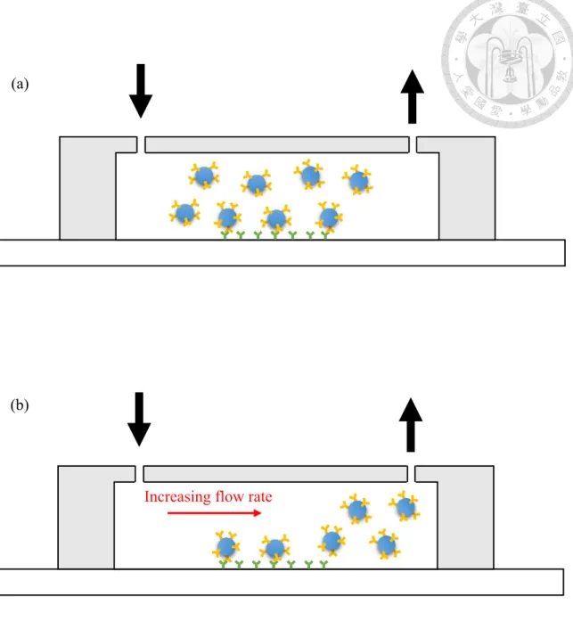
Figure 3-1 (a) Schematic diagram of microbeads in the microchannel for immobilization. Inject microbeads and stop pumping for immobilization. (b) After immobilization, increase the flow rate to wash away the microbeads attached on the surface. ... 17

Figure 3-2 Forces and torques acting on a sphere in shear flow ... 19

Figure 3-3 Schematic diagram of contact area ... 22

Figure 3-4 Force acting on the beads as it detached. ... 24

Figure 3-5 Schematic diagram of the contact area between microbeads and the substrate surface. ... 24

Figure 3-6 Adhesion force acting on the contact area of the bead in circular coordinates.25 Figure 4-1 Fabrication process of silicon mold for microchannel by lithography and ICP etching. ... 29

Figure 4-2 The microscope image of the microchannel silicon mold after Teflon coating. ... 30

Figure 4-3 Assembly of the microchannel holder ... 32

Figure 4-4 Acrylic holder with micrchannel and tube. ... 33 Figure 4-5 The seal ability test setup. ... 34 Figure 4-6 Flow chart of antibodies conjugation process. ... 36 Figure 4-7 Aggregation occurred when insufficient or excess antibodies was added. ... 39 Figure 4-8 Aggregation turned to dispersion after antibodies concentration was

optimized. ... 39 Figure 4-9 Flow chart of NHS-ester group contained polymer film chemical vapor

deposition. ... 41 Figure 4-10 Schematic diagram of detachment experiment setup. ... 43 Figure 4-11 (a) Image of the microchannel under inverse microscope. (b) Image

process using ImageJ which defines the pattern of the microbeads. ... 43 Figure 5-1 SEM image of microbeads. (a) Bare microbeads; (b) Microbeads coated

with rabbit IgG. ... 46 Figure 5-2 Specific binding test. Microbeads coated with rabbit IgG were injected

into the microchannel coated with anti-rabbit IgG for specific binding.

And microbeads coated with BSA were injected into the microchannel coated with anti-rabbit IgG for non-specific binding. ... 47 Figure 5-3 Experimental percentage of the microbeads remaining as a function of the flow rate. ... 48 Figure 5-4 Average experimental percentage of the microbeads remaining as a function of the flow rate with error bar. Regression line and error regression line are plotted too. ... 49 Figure 5-5 Calibration curve for labeled rabbit host IgG. ... 51 Figure 5-6 Relative average experimental percentage of the remaining microbeads as a function of the flow rate with error bar. Regression line and error

regression line are also plotted. ... 53

LIST OF TABLES

Table 4-1 Parameters for SPR 220-7 photoresist in lithography process ... 30 Table 5-1 Comparison of different methods of measuring protein-protein interactions. 54

Chapter 1 Introduction

1.1

1.1.1 Acute coronary syndrome

There are more and more people suffering from cardiovascular disease, generally referred to conditions that involve narrowed or blocked blood vessels that can lead to a heart attack, chest pain (angina) or stroke [1]. With increasing salt or fat consumption, people nowadays have increasing probability of having cardiovascular disease. Acute coronary syndrome (ACS), clinical presentation of myocardial ischemia, occurs when heart muscles lack of oxygen because of narrowed or blocked blood vessel. There were more than 1.1 million patients with acute coronary syndrome (ACS) in U.S in 2010 [1], and about 114,000 people go to hospital because ACS in UK each year [3].

ACS can be divided into ST-segment elevation myocardial infarction (STEMI), non–

ST-segment elevation myocardial infarction (NSTEMI) and unstable angina according to its different symptoms, electrocardiography (ECG) and enzymes concentration. In clinical, there is a series of examination to determine ACS including electrocardiography and different kinds of enzymes. In particular, enzymes detection takes a long time and the patient with ACS must be sent to the hospital to do such examination before being arranged to the next treatment. However, it is always very urgent for an ACS patient to arrive at hospital. Therefore, more and more laboratories aim to develop biosensors to detect the enzymes concentration in blood quickly and easily.

1.1.2 Biomarkers

Injured cardiac muscle release proteins and enzymes known as cardiac biomarkers into the blood. In clinical, biomarkers for diagnosis ACS are CK-MB, myoglobin and cardiac troponin. The timing of release of various biomarkers after acute myocardial infarction is shown in Figure 1-1. When acute myocardial infarction (AMI) occurs, [3]

CK-MB rises to a peak of 2 to 5 times the upper limit of normal (ULN: define as the 99th percentile from a normal reference population without myocardial necrosis; the coefficient of variation of the assay should be 10% or less), and returns to normal after about 2 days. Myoglobin is the earliest rising biomarker; however, it returns to normal concentration very fast, typically in 2~3 days after AMI. Troponin rises to different levels when large infarctions and small infarctions happened. For small myocardial infarction, as is often the case of NSEMI, troponin shows a small elevation. However, for large myocardial infarction, as is often the case of STEMI, troponin rises to more than about 13 times of CK-MB and lasts for about three days. Further, the troponin level may stay elevated above the ULN for 7 days or more after AMI. Because the concentration level of troponin is high and lasts for a long time for large myocardial infarction, the detecting will be easier and the risk of misjudgment is low. Therefore, troponin is the most important biomarkers to be monitored for a severe ACS patient.

1.1.3 Cardiac muscles and troponin

Cardiac muscle is one of three major muscles in human body; the others are skeletal and smooth muscles. Cardiac muscle can not be controlled by brain, so called involuntary muscle, but can coordinate contracts for heart to pump blood to the whole body for oxygen supply. Like most other tissues in body, cardiac muscles need blood to deliver oxygen and nutrients and to remove waste products. The artery which supplies blood to cardiac muscles is called coronary artery. If the coronary arteries became narrowed or even blocked, the cardiac muscles damaged and reduced the ability to pump blood efficiently due to the lack of oxygen supplied. Furthermore, sever blockage in coronary artery will lead to cardiac muscles necrosis. When cardiac

Figure 1-1 Timing of concentrations of various biomarkers released after acute myocardial infarction [3].

blood. And that is why cardiac troponin can be one of the cardiac biomarkers for diagnosis.

Cardiac troponins include three different proteins: troponin-I (TnI), troponin-T (TnT), and troponin-C (TnC). As shown in Figure 1-2 [5], all of them act as key roles in cardiac muscle contraction. They act together as a complex in inhibiting the binding of myosin to actin strands. TnT acts as a linker between troponin complex and myosin, TnI blocks the binding site between myosin and actin; TnC binds with calcium ion and then performs conformal change to move TnI away from the binding site. Therefore, the muscles can do contraction.

Figure 1-2 Proteins comprise cardiac myofilaments [5].

According to Jesse. E (1993) [6], cardiac troponin-I (cTnI) is highly specific for myocardial injury. Therefore, it is a good biomarker for ACS. In the past, CK-MB was the main detection biomarkers in clinical. However, it increases not only because of the cardiac muscles injured, but also skeletal muscles, causing diagnostic confusion.

Today, more and more research has shown that cTnI is a better cardiac biomarker because of its specificity in heart [7]. The normal concentration of cTnI in healthy human is below 0.4 ng/mL. The concentration greater than 2 ng/mL indicates high risk of cardiopathy [8].

1.1.4 Biosensors detecting cTnI biomarkers

Due to more and more people suffering from ACS, there are a lot of researches in developing biosensors to detect cardiac biomarkers. For practical usage, the essentials of biosensors are portability, convenient execution, rapid detection, high sensitivity, and low cost. Over the last decades, biosensors using different methods to achieve these characteristics have been developed. In general, they can be roughly divided into optical biosensors, electrochemical biosensors and transistor biosensors. For optical biosensors, such as enzyme-linked immunosorbent assay (ELISA) and surface plasma resonance (SPR), are the most common methods to sense the biomarkers concentration.

For ELISA based biosensor, its limit of detection (LOD) concentration can be as low as 0.03 ng/mL [9]. However, it takes about 5 hours of analysis time. For SPR techniques, the sensing time can be shortened for real-time detection; in addition, its LOD concentration can reach 0.07 ng/mL [10][11]. But it is high cost and needs expensive analysis equipment so it is difficult to be applied in point-of-care system.

impedance spectroscopy (EIS), LOD concentration were reported to be 1 ng/mL and 0.2 ng/mL. For transistor biosensors, according to [12], grapheme-based field effect transistor has been reported to have LOD of 0.04 ng/mL.

1.1.5 Antibody and aptamer

Most of biosensors use ligands to capture cTnI. The most common ligand is antibody which binds to its antigen specifically. Normal antibody identification process starts with an animal immune system and the generation process must be done in vivo. Therefore, antibody production is expensive and time-consuming. In contrast, aptamer can be identified in vitro that does not depend on animals, cells, or even in vivo condition [13]. Because animals and cells are not involved in generation process, the toxins and some unwanted molecules can be easily controlled. Therefore, high affinity aptamers can be produced.

The method to generate aptamers is called systematic evolution of ligands by exponential enrichment (SELEX), first reported by C. Tuerk et al. in 1990 [14].

Figure 1-3 shows the schematic process of SELEX [15]. At first, random nucleic acid source with target molecules was incubated. Second, unbound molecules were separated form bound molecules. Then, the bound nucleic acids were eluted and amplified by polymerase chain reaction (PCR). The process above were repeated for six to twelve cycles to obtain desirable aptamers with high purity. The development of SELEX techniques makes it possible to produce aptamers recognizing virtually any class of target molecules with high efficiency and low cost. In addition, SELEX techniques produces high specificity and affinity aptamers because the repeat cycles for recognizing target in process. In recent years, many literatures have reported that aptamers have better affinity than antibodies and claimed that aptamers are better candidates in immunobiosensors. In transistor-based biosensors, the shorter length of

aptamers makes it more sensitive than antibodies as ligands. Today, more and more biosensors using aptamers as ligands are developed.

1.2 Binding force between aptamer and target molecule

Aptamers are short, single strands of DNA or RNA with 3-dimentional structures that facilitate specific binding with their targets such as small molecules, DNAs, proteins or cells. Similar to antibodies, aptamers recognize their targets by 3-dimentional structures like Fig 1-4 shows [16]. Once recognizing their targets, aptamers bond to them by complementary RNA base pair which creates secondary structures such as short helical arms and single stranded loops. Combination of these secondary structures to their targets results in the formation of tertiary structures that

Figure 1-3 Schematic process of SELEX [15].

allows aptamers to bind to their targets via van der Waals force, hydrogen bonding and electrostatic interaction [17]. As the tertiary structures form, aptamers fold into a stable complex with the target. This complex has strong interaction force so it’s not easy to break the binding, making aptamer a good ligand with high binding affinity.

1.3 Motivation

The interaction force in aptamer-target complex is an important factor for understanding the recognition process. Further, the quantification of this interaction force is a key data for developing biosensors that use aptamers in microfluidics system.

Therefore, a lot of literatures have reported some methods to measure the binding force between this kind of ligands and receptors. Because there are many different kinds of forces in the aptamer-target complex, it’s still an unsolved problem about clarifying the interaction in detail. Based on the project which developed a transistor based biosensors in our laboratory [12], we focus on the binding force between cTnI and its aptamer in this article and quantify the interaction force by hydrodynamic shear assay in a microfluidic system. In the project, the biosensor is integrated with a microchannel

Figure 1-4 3D structures formation of aptamer and target binding [16].

and in which blood with biomarkers, cTnI, will flow into the channel by capillary force and go through detection area. The flow rate of the blood in the channel is important because the shear force of the fluid may be too strong so that the aptamers cannot capture the cTnI. As the result, the detection sensitivity decreases and the sensor performance will not reach the expectation. To optimize the flow rate of the blood in the channel, the interaction forces between cTnI and its aptamer are extremely important; hence it is necessary to investigate the binding force for developing the biosensors in the future.

In addition, the biosensors will detect not only one kind of biomarkers in our future development. Therefore, it is important to develop a method to measure the binding force between different kinds of ligand and receptors quickly and easily.

Chapter 2 Literature review

2.1 Binding force measurement using AFM

Atomic force microscopy (AFM) has been developed for few decades and used widely for scanning images in nano and micro scales. With a cantilever beam probe, AFM scans the sample surface by tapping or contacting and detects the force and the displacement of the cantilever beam. It then reconstructs the topography of the samples.

In 1994, Florin et al. used AFM to measure the specific interaction between biotin and avidin [18]. AFM probe with nitride tip was functionalized with avidin first. It then contacts with a biotinylated agarose bead and measures the force and the displacement of the beam, as shown in Fig 2-1. In Figure 2-1, the horizontal line means no forces acting on the cantilever beam as the tip approaches the surface. Suddenly, there is a compressive force acting on the tip when it contacts with the surface. In the retraction process, the adhesion force between bead and tip results in a deflection of the cantilever beam toward the bead. With increasing bend of cantilever, the tension force on the adhesive bond between bead and tip increases until the bond breaks. When the bond between biotin and avidin breaks, a sudden step occurs, which shows the maximum adhesion force between biotin and avdin in the retraction process. This condition allows only a limited number of molecular pairs to interact. The force required to separate the biotinylated agarose bead and the avidin coated tip was quantized in integers multiples of 160 ±20 piconewtons. In 1994, Lee et al. measured the force between two complementary DNAs using AFM [19]. As the reported results, the adhesive forces are 1.52, 1.11, and 0.84 nN, which are associated with 20, 16, and 12 base pairs of complementary DNAs separately.

Besides DNA and protein interaction, specific antibody and antigen interaction was investigated by Dammer et al. in 1996 [20]. In addition, primary and secondary antibody interactions and aptamers interactions were studied by Lv in 2010 [21] and Nguyen in 2011 separately [22]. Though a lot of different ligands and receptors have been discussed, they all had a same problem: it is hard to measure one pair of ligand and receptor directly at the same time. Always, there are multiple pairs of interactions between tip and sample surface in measurement because the tip of the probe is still too large compared to antibody, protein or DNA. However, it is still the most common way to measure the molecule interactions.

Displacement Force

Figure 2-1 Force and displacement relationship when AFM tip approaches to and retracts from the target protein [18].

2.2 Hydrodynamic shear assay

Though the interactions between ligands and receptors can be measured directly using AFM, there are some literatures which reported to measure the interactions by hydrodynamic shear assay because it needs expensive instruments and well controlled environment to reduce noises to measure the binding force using AFM. In 1990, Roberts et al. had tried to model the cell adhesion by conjugating beads to antibodies and then adhered them to surface-coated complementary antibodies. To investigate the interactions between two antibodies, they conducted beads detachment experiment in a radial flow device [23]. Schematic diagram of the radial flow device is shown in Figure 2-2. The fluid is injected into the radial discs through the tube in the middle of the device. Because the cross-sectional area of the flow increases with radial distance, the flow velocity and the shear force decrease. Therefore, within a circular zone around the inlet where the shear forces are higher, particles are swept away. However, within the outer zone where shear forces are smaller the beads can adhere. There is a boundary between these two zones, and the radius marked this boundary is defined as critical radius. The reported mathematical model interprets the experiment data and analyzes the adhesion between ligands and receptors. DNA binding was investigated with hydrodynamic flow in 2006 by Zhang et al. [24]. Similarly, beads coated with DNA specifically adhere to the surface with complementary DNAs; however, the whole device was a parallel plate flow chamber. The flow was controlled with a syringe pump, and the detachment experiment was observed with a converted microscope.

The interactions between the ligands and receptors were analyzed in these two literatures, but none of them had quantified the binding force. Lorthois et al.

investigated Fibrin/Fibrin-specific molecular interactions in 2001 [25]. With some

critical assumptions, Lorthois modeled the bond between fibrins as Hookean springs and calculated the binding force of the DNA pairs, suggesting that this force is about 400 pN.

Since microfluidics emerged in 1980s, precise control of small volume fluids makes it possible to reduce the cost and time of reaction in biological science. Further, the microscale fluids form stable laminar flow in microchannel naturally so the flow field can be easily controlled. With many advantages of microfluidics, a lot of researches have realized hydrodynamic shear assay in microfluidic systems.

Yokokawa et al. measured the adhesion force between kinesins and microtubule using hydrodynamic force produced by microfluidic flow in 2011 [26]. The microchannel is

Figure 2-2 Side view of radial flow device for detachment experiment [23].

fabricated by the poly(dimethylsiloxane) (PDMS) using casting method and held by aluminum plate holder. Microtubule is immobilized on the bottom of the channel, and the beads coated with kinesins adhered to it. Just like the literature above, the device was linked to syringe pump to perform detachment experiment. As the fluid force exceeded the adhesion force between kinesins and microtubule, the beads were swept away. In addition, the ATP was added into the fluid to decrease the binding strength between kinesins and microtubule. As the results, the binding forces are 362.9 pN and 31.3 pN for conditions of ATP absence and ATP presence separately.

There are same problems in hydrodynamic assay: there are multiple bonds between one bead and the surface. Binding density estimation may be a good solution. The contact area of the bead can be calculated; therefore, the bond numbers between bead and the surface can be estimated with binding density. Today, a lot of efforts are taken to measure single bond between ligand and receptor; however, no good methods can investigate the binding interactions with single bond.

2.3 Other methods to study the interaction between ligands and receptors

Except for the two methods mentioned above, there are other methods to study the interactions between specific ligands and receptors, such as unbinding cells by two micropipettes, optical tweezers method, centrifugation method and magnetic forces method etc. [27]. In 1991, Evans et al. first used two micropipettes to unbinding two capsules with adhesion molecules [28]. Markel et al. measured the unbinding force between biotin and streptavidin by conjugated them to two capsules separately. With the method like Evans, capsules sucked by two micropipettes were moved away slowly

and the force was measured as capsules separated. [27][29]. The biotin-streptavidin unbinding force was about 50 pN. For optical tweezers method, Nishizaka et al.

measured the unbinding force between actin filaments in 1995 and the unbinding force was 9.2 ± 4.4 pN [30]. In 1996, Miyata et al. reported that the unbinding force measured by optical tweezers between actin and skeletal muscle α-actin was about 18 pN [31].

With the development of biotechnology, the interactions between different kinds of ligands and receptors become more and more important. A lot of different methods to investigate this kind of molecular interactions have been developed. In this thesis, we will focused on hydrodynamic shear assay and measure the aptamer-cTnI binding force by this method.

Chapter 3 Principle and theoretical model

3.1 Measurement principle

In order to investigate the interaction forces between cTnI and its aptamer, a hydrodynamic shear assay was implemented in our experiment. We have an idea about measuring the binding force between cTnI and its aptamer by fluidic force.

However, the cTnI and its aptamer are too small to calculate the forces acting on them.

Therefore, we induced a spherical microbead as a medium to transport the force from the flow to the cTnI-aptamer complex. The model about the hydrodynamic shear load acting on a sphere attached to the plate surface has been well developed by O’Neill [32]

and Goldman [33]. Therefore, the force acting on the bead can be calculated easily.

Further, the adhesion force of the bead contributed by the ligand-receptor complex can be modeled, so the binding force and the unbinding force of the cTnI and its aptamer can be calculated. The adhesion force model of the microbeads carrying with cTnI-aptamer complex will be explained later. To realize the hydrodynamic shear assay, a microfluidic system was used in the experiment. The system consists of a strait rectangular microchannel, and the bottom of the channel was coated with aptamers.

The microbeads coated with cTnI will be injected into the channel, and the cTnI on the beads will be captured by the aptamers on the channel surface (Figure 3-1(a)).

Therefore, the microbeads will attach to the channel surface and can be observed by an inverse microscope. Than the fluid will be injected into the micrchannel to wash the beads away. More and more beads will detach with increasing flow rate, and the detachment results will have further proces to calculate the adhesion force of the beads (Figure 3-1(b)). Applying the model about the adhesion, the binding force of the cTnI and aptamer can be investigated finally.

(a)

Figure 3-1 (a) Schematic diagram of microbeads in the microchannel for immobilization. Inject microbeads and stop pumping for immobilization. (b) After immobilization, increase the flow rate to wash away the microbeads attached on the surface.

Increasing flow rate (b)

3.2 Hydrodynamic shear load on microsphere

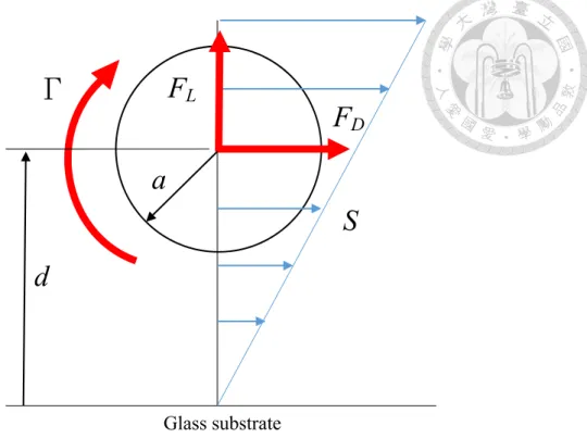
The schematic model of shear load acting on sphere in flow is showed as Fig 3-2.

Because there are cTnI-aptamer complexes between the microbead and the substrate surface, we assume that the bead has few nanometers of distance from the surface. In the rectangular microchannel, the velocity gradient caused by non-slip boundary layer leading to the shear rate, S, was showed as Fig 3-2. We applied the model from Goldman [33] which described a similar situation, and the model has been used successfully by R. Yokokawa [26] previously. From this model, the microbead is applied with three forces by the shear flow, the drag force, the lifting force and the torque. They are shown as below:

6 *

D D

F = πμadSF (2.1)

3 *

4 a Sπμ

Γ = Γ ^(2.2)

9.257 2 Re

FL = ×μa S (2.3)

in which, FD is the drag force, FL is the lifting force, is the torque contributed by shear flow, μ is the fluid viscosity, a is the bead radius, d is the distance from channel surface to the bead center, Re is the Reynolds number and S is the shear rate in the flow. FD*

and ^* is the non-dimensional parameter as a function of d/a. The geometry scale is extremely small in microchannel, leading to very small Reynolds number. As a result, the lifting force, FL, is about 2 orders smaller than FD and . Hence, FL can be neglected in computation.

The shear rate S in rectangular channel can be calculated by the equation below:

2

S 6Q

= h w (2.4)

in which, Q is the flow rate, h is the channel height and w is the channel width. By applying S ^6Q₂

= h w into Equation 2.1 and 2.2, the drag force and the lifting force become

*

36 2

D D

F Q ad F

πμ ^h w^

=   ^(2.5)

3

*

24 a2

Q h w πμ ^{ }

Γ =  Γ

  (2.6)

According to Goldman [33], the non-dimensional parameter FD* and ^* are, respectively,

* 9

D 1

F  a

= +   ^(2.7)

Glass substrate

S d

a

Γ F

F

Figure 3-2 Forces and torques acting on a sphere in shear flow

3

* 3

1 16 a d

Γ = −     (2.8)

By applying Equation 2.7 and 2.8 into Equation 2.5 and 2.6, the equations become:

2

36 1 9

D 16

ad a

F Q

h w d

πμ ^{   }

=   +    (2.9)

3 3 2

24 1 3

16

a a

Q h w d

πμ ^{    } Γ =   −   

   

   ^(2.10)

As the result, we can calculate the drag force and the torque acting on the sphere with flow rate, dimensional parameters and fluid viscosity.

3.3 Theoretical model

With the equations above, we can calculate the drag force and the lifting force acting on the microbead in the shear flow. Here, we are going to model the ligand-receptor complex and the microbead to investigate the situation when the beads detach and the ligand-receptor complexes break. Before modeling, we have some vital assumptions as below:

1. The ligand-receptor complex is modeled as linear spring.

2. All the ligand-receptor complexes between each microbead and the surface are equally stressed.

3. The microbeads were coated with ligands uniformly.

Because it is too complicated to model each bond with different strains when the microbeads are swept away, the assumptions above are necessary. In addition, it is hard to count the numbers of bonds formed as the microbeads attach to the surface.

With the assumption 3, we can calculate the numbers of bonds with contact area and the

bond density.

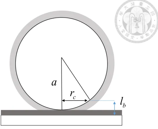
The contact area is a key parameters in our model, which is defined as the area where has ligand-receptors bonds. According to S. Lothois [25], the schematic diagram is showed as Figure 3-3. Because the ligand-receptor complexes are too small in comparison with the microbeads, there are many bonds formed between one bead and the surface. All the bonds between the bead and the surface contribute the adhesion, so the contact area should include the place where the bonds exist. Since the ligands on the microbead are coated uniformly, it is obvious that the contact area is a circle.

Here, we assume that the bonds length, lb, the radius of the microbeads, a, and the radius of contact area, rc. From Figure 3-3, the relationship of them can be showed as below:

( )

2 2

b c

a = a l− +r (2.11)

Furthermore, the radius of contact area can be derived from Equation 2.11 as

c 2 b

r = al (2.12)

As the radius of the microbead is known and lb can be estimated, the radius of contact area can be easily calculated. Since lb is the bond length, it can be estimated by the sum of the ligand and receptor length.

Since we have the contact area, the theoretical model can be established as Figure 3-4 shows. When the microbeads were dragged by the flow toward the outlet of the channel, it is assumed that the bond which is modeled as a linear spring is stretched at an angle α (Figure 3-5). The forces acting on the sphere are shown in the Figure 3-4.

We assume the torque is referred to the front edge of the contact area, as point I shown in Figure 3-4, and the adhesion force can be calculated by the equilibrium of the force acting on the sphere and the torque at the point I. The equilibrium equations are

Force equilibrium:

adh D L 0

F +F +F +W =

(2.13)

r c

l b

a

Figure 3-3 Schematic diagram of contact area. The lb is the characteristic thickness of the bond. The characteristic thickness of ligand and receptor are represented in light gray and dark gray.

Torques equilibrium:

adh FD a W a 0 Γ + Γ +   × + × =   

(2.14)

in which Fadh is the adhesion force acting on the sphere contributed by the bonds, W is bead weight, and adh is the torque contributed by the adhesion force. Since the ligand-receptor complexes are modeled as linear spring, the adhesion forces contributed by the bonds can be expressed as:

adh c

F =A Ckλ (2.15)

in which, Ac is the contact area, C is the binding density in unit area, k is the modeled spring constant, and λ is the modeled spring elongation.

As the Figure 3-6 shows, the torque contributed by the adhesion force can be calculated as

sin ( cos )

adh dFadh α rc r θ

Γ =



where r is the radius from dFadh to the center of the bead, and θ is the angle between dFadh to the x-axis.

By applying Equation 2.15, it becomes:

0^Ac sin ( cos )

adh Ck

λ α

θ

Γ =



With the circular coordinates shown in Figure 3-6, the Equation 2.17 becomes:

2

0 0^rc sin ( cos )

adh ^π Ck

λ α

θ

θ

Γ =

 

Integrating Equation 2.18 leads to

3 sin

adh πr Ckc λ α

Γ = (2.19)

Though the bond elongation and the bond spring constant are unknown, by modeling the bond as linear spring, the force contributed by the bond can be investigated by

F adh

F D

F L

Γ

I W

Figure 3-4 Force acting on the beads as it detached.

2 r

Figure 3-5 Schematic diagram of the contact area between microbeads and the substrate surface.

3.4 Critical flow rate

The critical flow rate which causes shear load sufficiently large to break the bonds and to detach the microbead is defined as critical flow rate. The bead size is Gaussian, as confirmed by the provider, Polysciences, Inc. As the result, the distribution of bond numbers is also Gaussian. As Gaussian distributions are symmetric around the mean value, the shear load to detach 50% beads is independent of the standard deviation of the distribution. Here, we defined the critical flow rate, Qc, as the value that causes 50% beads detachment. In fact, the critical flow rate is the necessary flow rate to detach the beads whose size is equal to the mean size of the distribution. Since we apply the Qc into the Equation 2.9 and 2.10, the drag force and the torque acting on the

θ

α r

r

F

Figure 3-6 Adhesion force acting on the contact area of the bead in circular coordinates.

bead when detachment occurred are show as below separately:

2

36 1 9

D C 16

ad a

F Q

h w d

πμ ^{   }

=   +    (2.20)

3 3 2

24 1 3

C 16

a a

Q h w d

πμ ^{    }

Γ =   −     ^(2.21)

3.5 Relationship between binding force and shear load

Since we have the shear load on the microbeads and the theoretical bond model above, we can calculate the binding force by applying the model and the load into the equilibrium equations. By applying the Equation 2.15 and 2.19 into Equation 2.13 and 2.14, the Fadh can be solved as

( )

2

2 2

1 ^{D c}

adh c c D

c D

aF Wr

F A Ck r Ck F

λ π λ r F^{+ Γ −}

= = = + (2.22)

Further, W can be replaced by ρVg, in which ρ is the density of the bead, V is the volume of the bead, and g is the gravity acceleration. The Equation 2.22 becomes:

( )

2

2 2

1 ^{D c}

adh c c D

c D

aF Vgr

F A Ck r Ck F

r F

λ π λ ^{+ Γ −}ρ

= = = + (2.23)

Now the adhesion force is a function of drag force and torque; the drag force and the torque are functions of critical flow rate as shown in Equation 2.20 and 2.21. The critical flow rate can be obtained by experiment, and the adhesion force of the bead can be easily calculated. Applying the binding density and the contact area, the bond numbers on the bead can be estimated, and so is the binding force per bond.

Chapter 4 Fabrication and experiment

4.1 Microfluidic system fabrication

The development of microfluidic system makes it possible to reduce the cost in biological research because the requirement for solvents, reagents and samples volumes are very small. With microfluidics, complicated process of biological assays performed in laboratory can be miniaturized on a small chip. Miniaturized versions of bioassays offer many advantages, including short reaction time, portability, low consumptions of power and potential for integrated with other miniaturized devices [34].

Further, with well-developed techniques of MEMS, the fabrication of microfluidic systems becomes easier and cheaper. Thus, the microfluidic systems are widely used in biological, medical research and bioassays.

Microchannel plays a key role in microfluidic systems, and lots of research have explored and developed the fabrication method of the microchannel. Based on well-established fabrication techniques in semiconductor industry, making microstructure molds on silicon wafer is the most common way to fabricate microchannel. Polydimethylsiloxane (PDMS) is one of the most widely used materials for microchannel in medical, biological and chemical applications because of its advantages of biocompatibility, low cost, easy molding into sub-micrometer features, chemical inertness, gas permeability and optical transparency for real-time optical detection [35]-[37].

4.1.1 Silicon Mold fabrication

In this article, the microchannel used in the microfluidic system was made from

sub-micrometers structures, the fabrication techniques of MEMS is the best choice.

The master mold used in this article was made from silicon wafer. Before fabrication, some process must be done to clean the silicon wafer. First, the inorganic contaminant on the wafer surface was removed by immersing the wafer in piranha solution (H2SO4 : H2O2 = 3:1) for 5 minutes, and then rinsed with deionized water, and dried with nitrogen gun. Than, the organic contaminant on the wafer was removed by acetone and isopropyl alcohol (IPA) bath for 5 minutes separately. Finally, the wafer was rinsed with deionized water and dried with nitrogen gun, and the clean process was done.

Before lithography process, the silicon wafer had to be modified in order to increase the adhesion between photoresist and the wafer surface. Hence, the wafer was soaked in BHF solutions for 5 minutes for modification. Again, the wafer was cleaned with deionized water and dried with nitrogen gun and it appeared that the silicon surface properties turned from hydrophilic to hydrophobic, and now the wafer was ready for lithography process. To define microchannel pattern, we spin coated about 6 μm positive photoresist (SPR 220-7) on the wafer first. Then, put the wafer with photoresist on the hotplate to soft-bake it for 90 s at 90 °C (Figure 4-1 (a)). The microchannel was patterned by exposing process under 3.9 mW/cm² for 70 s and then was developed in TMHA developer for 70s (Figure 4-1 (b)-(c)). After rinsed with deionized water and dried with nitrogen gun, the wafer was put on the hotplate for hard-bake at 90 °C for 15 minutes then the photoresist on the wafer was ready for mask for etching process. To etch the silicon wafer in high aspect ratio, we used inductively coupled plasma (ICP, Samco) etching for the process (Figure 4-1 (d)). Finally, the wafer was soaked with acetone and IPA to remove the photoresist (Figure 4-1 (e)) and immersed in piranha solution again for advance cleaning. The parameter of lithography process is listed in Table 3-1. In order to demold the PDMS replica easily,

a thin layer of Teflon (DuPont^TM Teflon AF, Dupont, Wilmington, Delaware, USA) was spin coated on the mold surface. Teflon was spin coated on the mold at 3500 rpm and heated at 90 °C for drying. The microscope image of the mold is shown as Figure 4-2, the surface coated with Teflon looks corrugated. However, the topography of the mold had been checked using Probe Type Surface Analyzer. The surface is still smooth and flat, the height of the corrugation is very small so can be ignored. The width and the height of the microchannels are 80 μm and 32μm separately which were measured by Probe Type Surface Analyzer.

(a)

(b)

(c)

(d)

(e)

Figure 4-1 Fabrication process of silicon mold for microchannel by lithography and ICP etching.

Table 4-1 Parameters for SPR 220-7 photoresist in lithography process

Process Parameters

Spin coating (3 steps)

(a). 500 rpm for 10 sec.

(b). 2000 rpm for 30 sec.

(c). 3000 rpm for 55 sec.

Soft bake 90 °C for 90 sec.

Exposure 3.9 mW/cm² for 70 sec.

Developing In TIMAH for 70 sec.

Hard bake 90 °C for 1min 15 sec.

Figure 4-2 The microscope image of the microchannel silicon mold after Teflon coating.

4.1.2 PDMS microchannel fabrication

After the silicon mold was fabricated, the PDMS microchannel can be made by replication process. Liquid PDMS prepolymer mixed with curing agent in 10:1 weight ratio was prepared before poured onto the mold. The liquid PDMS prepolymer and curing agent were fully mixed by a mixer, then placed in a vacuum chamber for degassing. After degassing for 30 minutes, the liquid PDMS mixture was poured onto the silicon mold and put into the vacuum chamber again to degas thoroughly for 1 hour.

If there were no bubbles in the liquid, then the mold was placed on a hotplate and heated at 70 °C for 3 hours to cure the PDMS thoroughly. And then the dried solid PDMS sheet was peeled from the mold carefully. There are 8 components on one sheet, and 4 microchannels on each component. Therefore, there are 32 microchannels being made in one batch. The peeled PDMS sheet have to be cut and punched to make the inlet and outlet holes.

4.1.3 Microfluidic system holder

The peeled PDMS replica has to be sealed with a substrate to form a channel.

Hydrophobic surface of PDMS can form reversible seal by conformal contact easily.

However, the adhesion is not strong enough to prevent liquid leakage at high pressure.

There are many methods to increase the adhesion between PDMS and glass, including chemical treatment, plasma treatment, and corona treatment [38]-[40]. The most common way is oxygen plasma treatment. According to Duffy et al. [41], PDMS and glass can be sealed by irreversible bonding with oxidation treatment, and both of them can be oxidized using oxygen plasma. Surface oxidation is believed to expose silanol groups (OH) at the surface of the PDMS layers and glass surface that when these

surfaces are brought together to form covalent siloxane bonds (Si–O–Si). Typically, such bonding can withstand 30-50 psi air pressure without breaking. All the methods above need to modify the PDMS and substrate surface. However, the glass substrate is specially prepared for antibodies immobilization in our research and can not be treated with oxygen plasma. In addition, the seal of the PDMS and the substrate need to withstand high pressure due to detachment experiment. Therefore, we designed a holder to hold PDMS replica and substrate together to seal the microchannel. The holder and the PDMS replica are shown in Figure 4-3, which is composed of a base to place the glass substrate and a cover to hold the PDMS replica.

Figure 4-3 Assembly of the microchannel holder

The holder base and the cover are made of acrylic by laser cutting. The holder holds the replica and substrate tightly with screw on four screw sockets. The photo of the holder is shown in Figure 4-4. The seal was checked by injecting dyed deionized water with increasing flow rate (Figure 4-5). The maximum flow rate could reach 80 μl/min without fluid leakage. The maximum flow rate in the test can detach the microbeads that attach to the surface with adhesion force of ~31.4 nN, which is much larger than the expected adhesion force of the beads in our research. In this test, we confirmed that the seal of the holder is good enough to against detachment.

Figure 4-4 Acrylic holder with micrchannel and tube.

Figure 4-5 The seal ability test setup.

Syringe pump

Microchannel

4.2 Preparation of IgG microbeads

4.2.1 Conjugation process

Carboxylated microbeads with 1 μm in diameter were purchased from Polysciences, Inc. The beads were made of polystyrene whose hydrophobic interactions with glass substrate contribute to their resistance to elastic and plastic deformation. Therefore, the beads will not deform when contact with surface and remain in their spherical shape. To confirm whether the detachment experiment setup can be used to measure the binding force, we first measured the binding force between rabbit IgG and goat anti-rabbit IgG, which has been investigated before. In addition, IgG antibodies is easier to acquire and cheaper than the cTnI so it is better for us to use IgG to optimize the concentration in conjugation process. In our research, we conjugated two kinds of proteins onto the microbeads which are bovine serum albumin (BSA) and rabbit IgG for non-specific binding and specific binding.

The carboxylic acids groups on carboxylated microbeads can crosslink to primary amines compounds with N-(3-Dimethylaminopropyl)-N-ethylcarbodiimide hydrochloride (EDC) and N-Hydroxysuccinimide (NHS) in aqueous condition. This method is called carbodiimide crosslinking chemistry and the detail of activation process was shown in Figure 4-6. EDC reacts with carboxylic acid group to form an active O-acylisourea intermediate (Figure 4-6-(b)) which is easily displaced by NHS in the reaction mixture. Actually, the O-acylisourea intermediate can crosslink with primary amino groups on the protein, but it is unstable in aqueous.

The intermediate easily hydrolyzes if it fails to react with primary amino groups.

Therefore, NHS is added to replace the intermediate from EDC to form a more stable amine reaction group. NHS-ester forms on the microbeads (Figure 4-6-(c)) as NHS replaces the intermediate from EDC and can be easily displaced by nucleophilic attack from primary amino groups on the protein (Figure 4-6(d)). With EDC and NHS, the carboxylic acid groups on the microbeads crosslink efficiently with primary amino groups on the proteins.

O OH

+NH ^N

Cl-

O HN

O

EDC NHS

N O

O O O

Protein

O

NH

+NH

N C

N Cl-

EDC

N O

O

OH

NHS IgG antibody

(a) (b) (c)

(d)

Figure 4-6 Flow chart of antibodies conjugation process.

Before conjugation process, the carboxylated microbeads had to be washed. First, we pipetted 5 μl of microbeads into a 1.5 ml centrifuge tube and then added 170 μl MES buffer. MES buffer was prepared by dissolving MES hydrate in deionized water at the concentration of 10 mM and followed by the introduction of NaCl to reach the concentration at 0.9 wt%. The solution was then adjusted to pH 5.5. The microbead suspension was centrifuged for 6 minutes, and the supernatant was carefully removed using a pipette. Next, we refilled the centrifuge tube with MES buffer to suspend the microbeads and repeated the process above for three times. Then the microbeads were ready for protein conjugation. Before the protein conjugation, a 200 mg/ml EDAC solution was prepared by dissolving 10 mg EDC in 50 μl MES buffer, and 120 mg/ml NHS solution was prepared by dissolving 6 mg NHS in 50 μl MES buffer. We added 20 μl EDC solution and 20 μl NHS solution in sequence into the microbeads suspension to activate the carboxylic acid group. The microbeads were sonicated for 15 minutes, and the excess EDC and NHS in the solution were removed by centrifuge. Then, we re-suspended the microbeads in 210 μl PBS buffer and added 10 μl rabbit IgG solution (1 mg/ml). The solution was sonicated for 15 minutes and mixed for 30 minutes. To block the unreacted group on the microbeads, excess BSA was added and mixed overnight. After removing the excess rabbit IgG and BSA and re-suspending microbeads in 400μl PBS buffer by sonication, the conjugation process was done.

4.2.2 Rabbit IgG conjugation optimization

Microbeads aggregation is a problem to be solved in the conjugation process.

The microbeads we bought from Polyscineces, Inc. is well dispersed in deionized water and PBS buffer because of the full surface charge on the beads. However, each steps

aggregation (Figure 4-7). This kinds of aggregation could be reversed by some methods. Sonication is one of them and that is why we sonicated the latex at each step.

However, some reasons may cause irreversible aggregation such as crosslinking between beads and beads by proteins. One protein will crosslink to two or more microbeads if insufficient protein is added in conjugation process. To avoid this kind of microbead aggregation, the volumes of rabbit IgG added into the latex for conjugation have to be optimized.

The amount of protein required to saturate the bead surface can be estimated by equations provided by Polysciences, Inc.:

Sat

S = 6 _P

S S

d C

ρ ^(4.1)

where SSat is the amount of representative protein required to achieve surface saturation, ρs is the density of solid sphere, ds is the mean diameter of solid sphere, and CP is the capacity of solid sphere surface for a given protein. For IgG with molecular weight about 150 kDa, the capacity CP is estimated as 2.5 mg/m². The diameter and the density of the microbead is 1 μm and 1.05 g/cm³. We prepared 5 μl microbeads in conjugation process, and the amount of rabbit IgG to saturate the beads is about 0.2 μg which is calculated by Equation 4.1. For optimization, we prepared 1 mg/ml rabbit IgG in PBS buffer and added different volumes of it in conjugation. From the computation above, only 0.2 μl of rabbit IgG would be enough. However, the results showed that the microbeads aggregated after conjugation. Thus we increased the volume added into the latex and found that 10 μl of rabbit IgG was enough to disperse the microbeads (Figure 4-8). There is about 20 μg rabbit IgG in the latex for conjugation, which is 100 times of estimated amount.

Figure 4-7 Aggregation occurred when insufficient or excess antibodies was added.

Figure 4-8 Aggregation turned to dispersion after antibodies concentration was optimized.

4.3 Preparation of Anti-IgG substrate

The glass substrate was coated with anti-rabbit IgG for specific binding with rabbit IgG. Glass wafer was cut into 21.7 mm X 25 mm pieces as substrate and cleaned thoroughly. Glass substrate was soaked in piranha solution for 5 minutes and rinsed with deionized water. Then immersed in acetone, IPA and deionized water for 5 minutes in sequence and dried with nitrogen gun. For protein coating, the glass surface had to be modified. Without any chemical treatment, the glass substrate was only chemical vapor deposited (CVD) with a layer of polymers contained NHS-ester group. The chemical vapor deposition polymerization process is shown in Figure 4-9.

4-N-hydroxysuccinimide ester-[2.2] paracyclophane was first sublimed; the resulting vapor was transferred into the pyrolysis zone and then then polymerized upon condensation to the cooled substrate surface [42]-[44]. The thickness of the CVD polymer was about 30 to 50 nanometers, and the NHS-ester group on it can easily form covalent bonding with primary amino group on the protein at room temperature in aqueous conditions. For anti-rabbit IgG conjugation, the antibodies was prepared at concentration of 10μg/mml in PBS buffer first. Next, we assembled PDMS replica and the glass substrate which had chemical vapor deposited with NHS-ester to be a microchannel, and injected anti-rabbit IgG (10 μg/mml) under slow flow velocity overnight. Then PBS buffer was injected into the microchannel to remove unbinding antibodies. At last, BSA solution was injected to block the excess NHS-ester group on the glass substrate followed by PBS buffer for removing unbinding BSA.

4.4 Experiment

4.4.1 Specific binding test

In order to confirm whether the microbeads were conjugated with rabbit IgG completely, the specific binding test was conducted. For specific and non-specific binding test, microbeads conjugated with rabbit IgG and BSA were prepared. Also the glass substrate coated with anti-rabbit IgG and BSA were prepared. Anti-rabbit IgG will catch the beads coated with rabbit IgG and form specific binding; in contrast, the beads coated with BSA will not be captured and most of them will be washed away under slow flow velocity. Only few of them will attach on the surface because non-specific binding. We injected both microbeads into two microchannel separately for the test and observed the amounts of the microbeads attached on the surface after 1 hour under very slow flow velocity.

4-N-hydroxysuccinimide ester-[2.2] paracyclophane

CVD

poly(4-N-hydroxysuccinimide ester-p-xylyene-co-p-xylylene) Figure 4-9 Flow chart of NHS-ester group contained polymer film chemical vapor deposition.