具有線性及接地調整方式之可變負重之靜平衡鉸接式平面操作器之設計

(1)

國立臺灣大學工學院機械工程學系碩士論文

Department of Mechanical Engineering College of Engineering

National Taiwan University Master Thesis

具有線性及接地調整方式之可變負重之靜平衡

鉸接式平面操作器之設計

Design of Planar Various-Payload Balanced Articulated Manipulators with Actuated Linear Ground-Adjacent

Adjustment

蔣瑋軒

Wei-Hsuan Chiang

指導教授：陳達仁博士 Advisor: Dar-Zen Chen, Ph.D.

中華民國 105 年 7 月

(2)

中文摘要

在本論文我們提出了一種可變負重之靜態平衡鉸接式操作器設計。透過重力和彈力位能的方程式，歸納出剛性矩陣(Stiffness Block Matrix SBM)來表現重力和彈力在各關節之間的相對位能，藉此求得重力和彈力位能作用於各關節之間的平衡方程式。並根據每一個彈簧安裝參數在平衡方程式中扮演的角色進行分類，可以將其分為用於平衡負重的安裝參數（Payload dependent parameter PDP）和與負重無

關的安裝參數（Payload independent parameter PIP），PDP 皆需要根據負重的改變來

調整其接點位置，PDP 調整裝置的設計即是用來調整 PDP。透過分析 SBM 中的平衡方程式，可以歸納出將 PDP 的安裝於地桿及線性調整的彈簧配置。操作器上所需的 PDP 的數量會隨著自由度增加而增加，藉此可以得知在不同可變負重的操作器上容許的彈簧安裝數量。對於不同彈簧安裝數量的操作器，可依據 PDP 和 PIP 之間的相互關係，透過適當的安排 PIP 來減少 PDP 的數量。另外，對於擁有複數

PDP 的操作器，其位移量能夠透過適當的 PIP 來等量化，藉此讓多個 PDP 安裝在相同的調整裝置上，將 PDP 調整器的數量減少至一個。最後，根據設計理論，以兩個自由度的可變負重之操作器作為說明範例，進行 PDP 調整位置及位能變化的分析，並製作出實體原型機，用來驗證及展示本研究的設計概念。

關鍵詞：可變負重、平衡、彈簧、接地、線性調整

(3)

ABSTRACT

Supporting different payloads has been shown to be effective for developing a multitasking manipulator. This paper presents a method for designing a static balanced articulated manipulator for sustaining various payloads. The balancing equations for the gravitational and spring elastic energies are developed using a stiffness block matrix, which represents interacting potential energies between the links. It is shown that the spring can be classified according to the role it plays in the balancing equations. Thus, the installation parameters can be divided into payload-dependent parameters (PDPs) and payload-independent parameters (PIPs). The admissible spring configurations for supporting various payloads are determined using the required number of PDPs, and PDPs adjustment devices are used to adjust PDPs while the payload changes. Base on the interrelation between PDPs and PIPs. The number of PDPs can be reduced through proper arrangement of PIPs. The displacement of different PDPs can be equalized to fit attachment points in the same adjustment device. Therefore, the number of PDP adjustment devices is minimized to one. 2-DOF various-payload balanced articulated manipulator is shown as illustrative example. A prototype is fabricated to demonstrate the various payload balancing method of this study.

Keyword: various payload, balanced, spring, ground, linear adjustment

(4)

List of Tables

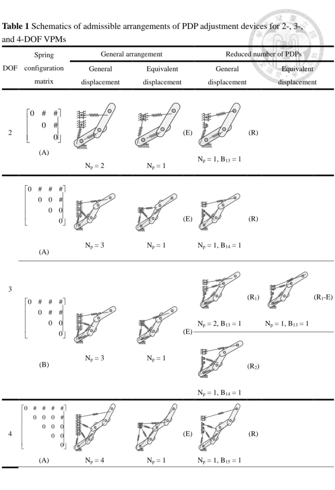
Table 1 Schematics of admissible arrangements of PDP adjustment devices for 2-, 3-, and

4-DOF VPMs ... 33

Table 2 Inertia and dimensional parameters of 2 DOF VPM ... 40

Table 3 Associated spring constants and attachment angles ... 41

Table 4 Installation parameters corresponding to different payloads ... 42

Table 5 Total potential energy with payloads of 0, 1, 2, and 3 kg, and the energy consumption for adjusting PDP to gain 1 kg of payload ... 45

Table 6 Inertia and dimensional parameters of 3-DOF VPM ... 45

Table 9 Total potential energy with payloads of 0, 1, 2, and 3 kg, and the energy consumption for adjusting PDP to gain 1 kg of payload ... 51

(7)

List of Figures

Fig. 1 Statically balancing parallelogram linkages [8] ... 2

Fig. 2 Statically balancing articulated manipulator [14] ... 2

Fig. 3 Self-adjusted mechanism for various payload [18] ... 3

Fig. 4 Mechanisms of energy free adjustment ... 4

Fig. 5 Design of variable gravity compensation mechanism [23] ... 5

Fig. 6 Gravity position of n-link articulated manipulator and changeable payload fitted at the end effector of link n and spring connected between link i and link k ... 9

Fig. 7 Definition of the direction of PDPs and proximal and distal PIPs. Schematic of a PDP adjustment device. ... 18

Fig. 8 Distribution features of the summation of the elastic SBM of ground-adjacent springs. ... 22

Fig. 9 Distribution features of nonzero terms in the elastic SBM with attachment point ɑ2q = r2 and attachment angle α2q = 180° (for q > 3). ... 25

Fig. 10 Arrangements for reducing the number of PDP adjustment devices ... 31

Fig. 11 Two-DOF, three-spring VPM with the minimum number of PDP adjustment devices with payloads of 0, 1, and 2 kg ... 43

Fig. 12 Simulated potential energy of 2-DOF, three-spring VPM with payloads of 1, 2, and 3 kg ... 44

(8)

Fig. 13 Three-DOF, five-spring VPM with the minimum number of PDP adjustment

devices with payloads of 1, and 2 kg ... 49

Fig. 14 Simulated potential energy of 3-DOF, five-spring VPM with payloads of 1, 2, and 3 kg ... 50

Fig. 15 Arrangement of pulley and wire construction ... 52

Fig. 16 Arrangement of routing and cable-loop-driven mechanism ... 53

Fig. 17 CAD of 2-DOF, three spring VPM ... 54

Fig. 18 Engineering prototype of 2-DOF, three spring VPM ... 55

Fig. 19 Guiding elements for installation parameters... 55

Fig. 20 Parallel and symmetric arrangement for pulley and wire ... 56

Fig. 21 Engineering prototype of lead screw and slider construction ... 57

Fig. 22 Cable-loop-driven mechanism ... 58

Fig. 23 Steps for changing payloads and adjusting PDP adjustment device ... 58

(9)

Chapter 1 Introduction

1.1 Background

Statically balanced manipulators maintain equilibrium in any configuration without actuators functioning. In recent years, several methodologies have been proposed to compensate for the weight of linkages. The counterweight method balances a manipulator by supplying a force in the opposite direction; however, this increases the system’s inertia [1].The spring-balancing method uses spring forces to compensate for gravitational forces;

consequently, the system’s inertia remains small [2-6].

1.2 Related works

One of the spring-balancing approaches is to use parallelogram linkages to ensure that vertical members exist at the end of each link; therefore, a multi-DOF manipulator can be considered a series of connected 1-DOF manipulators shown in Fig. 1 [7-9].

Agrawal et al. applied auxiliary parallelograms to a human upper arm orthotic device [10], human leg orthotic device [11], and assistive device for sit-to-stand tasks [12] to support people experiencing muscle weakness. However, auxiliary linkages may increase the inertia of the system and interfere with the motion of linkages.

(10)

Fig. 1 Statically balancing parallelogram linkages [8]

To improve these problems, Lin et al proposed stiffness block matrix method (SBM) to explore the interacting potential energies between links of multi-link planar articulated manipulators [13-17]. Therefore, those interacting potential energies can be compensated by the approaches without auxiliary linkages. Although the configuration of spring may be relatively complex, install locations of those springs can be derived easily.

Fig. 2 Statically balancing articulated manipulator [14]

With the increasing usage of support or assistive equilibrators, supporting various payloads has been shown to be effective for developing multitasking manipulators, such as robotic arms, surgical light assist devices, and monitor support devices. Therefore,

(11)

balanced devices that support various payloads have been developed. To maintain static balance, the spring configuration should be altered with different payloads. Nathan proposed a static balancer in which spring attachment points can be self-adjusted shown in Fig. 3 [18].

Fig. 3 Self-adjusted mechanism for various payload [18]

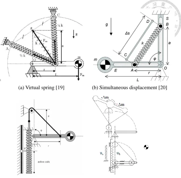
Herder et al. was focus on the design of adjustment method, and proposed several energy-free adjusting concepts such as virtual springs [19], simultaneous displacement [20], spring stiffness [21], and storage springs [22] shown in Fig.4 (a)-(d). However, energy-free adjustment methods should function with the weight arm locked at a preselected position.

(12)

(a) Virtual spring [19] (b) Simultaneous displacement [20]

(c) Spring stiffness [21] (d) Storage spring [22]

Fig. 4 Mechanisms of energy free adjustment

Takesue et al. focused on the spring configuration of variable gravity compensation mechanisms. Two types of springs with a 90° phase difference are used to compensate for variation in gravity without using wires shown in Fig. 5 [23]. Energy-free design is not concerned, and therefore, some energy may be allowed to compensate during the adjustment of the attachment points.

(13)

Fig. 5 Design of variable gravity compensation mechanism [23]

However, these methods are focused on the compensation of gravitational and elastic force between ground and ground adjacent link. Information about interacting potential energies between multi-links is not sufficient. The design of auxiliary linkages may be required to adapt those methods to multi-links manipulator. Therefore, this paper focuses on the spring configuration of multi-link planar articulated manipulators and estimation

of the energy consumption during adjustment.

1.3 Motivation and objectives

Since the various payload compensation mechanism has been explored for several years, however, the studies only focused on one DOF manipulator. Therefore, to use the manipulator more efficiently, the research for a high DOF of VPM is demanding. For this reason, the spring configuration of multi-DOF manipulators is explored in this study. Note that the energy free adjustment design is not concerned here.

The method proposed in this paper is based on the stiffness block matrix (SBM) approach

(14)

[15]. Previous studies have mainly focused on the compensation of fixed gravitational potential energy. Herein, however, the SBM approach is generalized for various payloads.

This paper explores the relation between spring installation parameters and the gravitational potential energy of the payload according to balancing equations of gravitational and elastic potential energy. The installation parameters that must be adjustable while payload changes are determined are called payload-dependent parameters (PDPs). By contrast, the installation parameters for fixed locations are defined as payload-independent parameters (PIPs). The general criteria for determining the admissible spring configuration for an n-link various-payload balanced articulated manipulator (VPM) on the basis of the required number of PDPs are proposed. The contributions of the attachment angles and attachment points of the spring installation to static balancing are explored. The PDP adjustment device is determined to be a slider that can lock at any position along the perpendicular slide rail. Therefore, the number of PDPs indicates the number of adjustment devices that are adjustable while the payload changes.

On the basis of the interrelation between the PDPs and the PIPs, the displacement of the PDPs can be expressed as a linear equation of the PIPs. The number of PDPs can be reduced through an associated PIP connected between the ground and the joint. The feasible reduced number of PDPs is determined according to the spring configuration.

(15)

For a VPM with multiple PDPs, the displacement of the PDPs can be equalized by installing associated PIPs at the distance with their spring constant ratio. Therefore, these PDPs can be fitted on the same PDP adjustment device to minimize the required number of adjustment devices to one. Similarly, the feasibility of the equivalent design is determined according to its spring configuration. The energy consumption during the adjustment is estimated base on the simulation results of the variation of total potential

energy for various payload.

1.4 Overview of the dissertation

The remainder of this paper is organized as follows. Section 2 introduces the formulation of the elastic potential energy and gravitational potential energy represented by the SBM. On the basis of the summation of the gravitational and elastic SBMs, the spring installation parameters are classified according to the role they play in the balancing equations. Section 3 describes the general criteria for the admissible spring configuration for an n-link VPM according to the number of required PDPs and balancing equations derived from the nonzero component matrices of the summation of the gravitational and elastic SBMs. The formulation of the PDPs and PIPs is then explored according to the spring configuration. In Section 4, because the displacement of the PDPs is expressed as an equation of the PIPs, the additional criteria for the installation of PIPs

(16)

are determined to reduce and equalize the nonzero displacement PDPs. Section 5 presents the derivation of a planar 2-, and 3-DOF VPM as design examples. The static equilibrium of quasistatic continuous motion is verified. Moreover, arrangement of standard springs, the method of reducing spring elongation, and the procedure of the adjustment of PDPs are explored for the engineering prototype of 2-DOF VPM. The energy consumption is estimated accordingly.

(17)

Chapter 2 Characteristics of SBM

2.1 Coordinate system of SBM

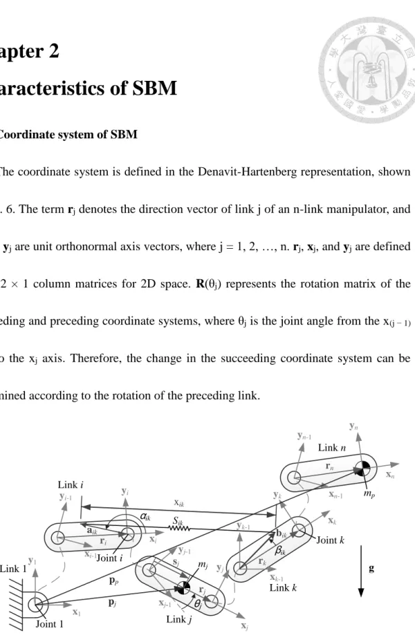
The coordinate system is defined in the Denavit-Hartenberg representation, shown in Fig. 6. The term rj denotes the direction vector of link j of an n-link manipulator, and xj and yj are unit orthonormal axis vectors, where j = 1, 2, …, n. rj, xj, and yj are defined to be 2 × 1 column matrices for 2D space. R(θj) represents the rotation matrix of the succeeding and preceding coordinate systems, where θj is the joint angle from the x(j − 1)

axis to the xj axis. Therefore, the change in the succeeding coordinate system can be determined according to the rotation of the preceding link.

Link i

Link 1

Link j

Link k rk

rj

ri

bik

aik

β_ik αik Sik

xik

pj

x1

xi-1

xi

xj

xk-1

xk

xn-1

xn

yn

yn-1

yj-1

yk

yk-1

yj

xj-1

yi

yi-1

y1 sj

g mp

pp

mj

rn

Joint 1

Joint i

Joint k

θj

Link n

Fig. 6 Gravity position of n-link articulated manipulator and changeable payload fitted at the end effector of link n and spring connected between link i and link k

(18)

2.2 Characteristics of gravitational SBM

The SBM method was proposed for analyzing a static balanced articulated manipulator with fixed potential energy in previous studies [16]. The term mj represents the mass of link j; pj represents the position vector of the mass center aligned along the line passing through the joints of links; g represents the gravitational acceleration; and I’

represents the rotation matrix that rotates 270°. The gravitational potential energy U^g is expressed as

j n

j j

g



m g^Tp



2

U (1)

where

n r j

s ^j

v v j

j j j

v v j

j 2,...,

1

1 1

1











 

^







r r

r s

p (2a)

1 1

1 1 0

1 0 2

3 x x Ix

R

g   



 



 

 



 



 g   g g

(2b) where rj is the direction vector of link j, and sj is the vector from joint (j – 1) to the mass center of link j, and its orientation is the same as that of direction vector rj. In addition, rj

and sj are the magnitudes of rj and sj, respectively.

In this study, various payloads are embedded at the end effector of the articulated manipulator. Therefore, the gravitational potential energy consists of the gravity of links and various payloads. mp represents the mass of the payload, which may vary, and pp

(19)

represents the position vector of various payloads fitted at the end effector of link n. The gravitational potential energy U^g is rearranged as

j n

j j p

p

g m g^Tp



m g^Tp







2

U (3)

where





 ⁿ

v v p

1

r

p (4)

According to Eqs. (1–4), the SBM representation for the gravitational potential energy can be obtained as

   



































n uv

n n

v

v T v v v g T

r r x G r r x r

G r r G r

T



2 1 2

1

1 1 1

1 2

U 1 (5)

where [Guv] is called the gravitational SBM, and its elements Guv are called gravitational component matrices, which represent gravitational interacting potential energies between links u and v. Owing to its symmetry [18], Guv can be expressed as an SBM, as shown in Eq. (6), and only the upper triangular matrix is considered.

 















0 0 0 0

0

0 ₁₂ ₁ ₁













 _v _n

uv

G G

G

G (6)

(20)

The gravitational component matrices G1v are expressed as

 

^m ^v ⁿ

r m s m g W

m g

n

v j

j v

v v p v

p

v 2,...,

1

1   





  

















I I

G (7)

where Wv is the sum of the mass of links from links v to n. Each component matrix Guv

in the gravitational SBM represents the quantity of the gravitational effect that acts between the ground (link 1) and link v. Therefore, Guv has a nonzero element in only the first row (i.e., u = 1) of off-diagonal matrices, as shown in Eq. (6). According to Eq. (7), Guv is a function of the payload and mass property of links.

2.3 Characteristics of elastic SBM

The spring configuration matrix [Sik] represents the configuration of fitted springs in an n-link SBM. Sik = 0 denotes that there is no spring installed between links i and k, and Sik = # denotes that at least one spring is installed between links i and k.

The expression of elastic potential energy is suggested by Lee et al.[15]. A spring with spring constant k^ik, fitted between links i and k of an n-link articulated manipulator, is shown in Fig. 6. Assume that the springs used are zero-free-length springs, and the distance between two attachment points |xik| can be considered the elongation of the spring. The elastic potential energy can be expressed as

ik T ik ik

ik k x x

2

U  1 (8)

where

(21)



^









 ¹

1 k

i u

u ik

ik

ik b a r

x (9)

aik and bik are proximal and distal installation parameters, respectively. Their position vectors extend from the joints of links i and k to the attachment points of the spring, respectively, and they can be expressed as

   



 











1

1 1

1 1 1 1 1 1

r i a

i x a

a

i ik i

ik

k k k

k

ik

r R

x R x

R a



(10a)

 

_ik _k

k ik

ik r

b R r

b   (10b)

where R(αîk) and R(βîk) are 2 × 2 rotation matrices, and αîk and βîk are the attachment angles from ri to aîk and from rk to bîk, respectively. Notice the special case for springs with i = 1, as shown in Eq. (10a). x1 is the length of unit vector x1, hence, it equal to 1.

According to Eqs. (8–10), the SBM representation for the elastic potential energy can be obtained as

  































 ⁿ

v u

n ik uv

n v

ik v u ik

1 ,

2 1 2

1

1 2

U 1

r r x K r r x r

K

r   (11)

where [𝐊_uv^ik] is called the elastic SBM of spring Sik, and the elements 𝐊_uv^ik are called

elastic component matrices, which represent elastic interacting potential energies between links u and v. Because [𝐊_uv^ik] is a symmetric matrix, only the upper triangular matrix is

(22)

considered as represented in the following:

 



















0 K K K

K K

K

0 0

K

ik kk ik uk ik

uv

ik ik ik

iv ik

ii

ik uv















(12)

The off-diagonal terms of the elastic component matrices 𝐊_uv^ik (for u ≠ v) are

expressed as

 



 





































k v k i

r u k b

k i

v u k

k v i r u

b r k a

k i

v i r u

k a

ik k ik ik ik

ik ik k ik i ik ik

ik i

ik ik

ik uv

; 1 , ...

, 1

1 , ...

, 1 ,

;

1 , ...

, 1

;









R I

R R

K (13)

Similarly, the diagonal terms of the elastic component matrices 𝐊_uv^ik (for u = v) are expressed as

















 



 











 



 







k v r u

k b

k i

v u k

i v r u

k a

k ik ik ik

i ik ik

ik uv

I I

I K

2 2

1 ..., ,

1 (14)

Each elastic component matrix 𝐊_uv^ik shows the quantity of the elastic effect of the spring Sik between links u and v. Therefore, 𝐊_uv^ik has nonzero terms in the diagonal part of rows u to v and columns u to v, as shown in Eq. (12). Because the elastic potential

(23)

energy of the spring affects only the links that it spans over, the nonzero elements of 𝐊_uv^ik are within the range i ≤ u, v ≤ k. According to Eqs. (13–14), 𝐊_uv^ik is a function of the spring constant, ratio of the distance between the joint and the attachment point of the spring to the length of the links to which the spring is attached, and attachment angles.

2.4 Static balance of total SBM

The gravitational and elastic potential energies change with the relative angular displacement between links u and link v, as shown in Eq. (15). To keep the total potential energy unchanged regardless of the configuration of the manipulator, all component matrices between every two distinct links (u ≠ v) must be zeros.

 

v T u uv cos^¹ r r

 (15)

Because the gravitational and elastic potential energies both have the same form, the total potential energy [Tuv] can be expressed as the sum of the gravity and elastic SBMs, and Tuv denotes the total component matrices, which represent total potential energies between links u and v.

The gravity potential energy induces nonzero elements in the first row of Tuv (for u

= 1) only. The associated spring Sik (for i = 1) with nonzero elements in the first row is required to balance Guv (for u = 1). Therefore, the first row of the total component matrices can be expressed as

(24)

n

N v

k v v

v ₁ ¹₁ 0 2,...,

1 ^G 



^K  

T (16)

The gravitational component matrix includes the gravity of various payloads. To calculate the balancing equation of T1v as scalar, the ground-attached end of spring S1k

must be installed at angle α1k = 90° or 270°, and the link-attached end must be installed at angle β1k = 0° or 180°. Therefore, the rotation matrix I’ can be ignored during the calculation. The elastic component matrices 𝐊_uv^1k of spring S1k can be rearranged as





















 





 





k v k u

B k

k v

u k

k v u B A k

k v

u A

k

k k k

k k

k uv

; 1 , ...

, 2

1 , ...

, 2 ,

; 1

1 , ...

, 2

; 1

1 1 1

I I

K (17)

where A1k and B1k are determined to represent dimensionless installation parameters expressed as



_k



_k



_k



k

k α a α

x

A a ₁ ₁ ₁

1 1

1  sin   sin  (18a)

 

_k

k k

k r

B₁  b¹ cos ₁ (18b)

Considering the design parameters of spring S1k, there is one spring constant k1k and two installation parameters A1k and B1k. The installation parameter B1k is fitted in both first row and non-first-row component matrices, and it is attached to the link. Therefore, the adjustment of B1k would additionally influence the non-first-row component matrices and interfere with the motion of links. However, the installation parameter A1k is fitted in

(25)

first row component matrices only and is attached to the ground. Therefore, the adjustment of A1k can avoid these problems. Thus, the installation parameter A1k is determined to be adjustable for various payloads.

For the non-first-row elements of Tuv (for u ≠ 1), gravity has no influence but the ground-adjacent springs have elastic influence. Therefore, spring Sik (for i ≠ 1) must be installed to generate a counterbalancing force in the non-first-row parts to compensate for the influence of the non-zero elements of 𝐊_uv^1k (for u ≠ 1).

1

; 1 ,

1  0  





^uv^k



îkûv û ^v ândⁱ

uv NK NK

T (19)

Similarly, because the attachment angle of component matrix 𝐊_uv^ik (for i ≠1) is defined as β1k = 0° or 180°, the attached end of the counterbalancing spring Sik should be installed at angles α1k = 0° or 180° and β1k = 0° or 180°, so the rotation matrix I can be ignored during the calculation. The elastic component matrices 𝐊_uv^ik of the counterbalancing spring Sik can be rearranged as



































k v k i

u B

k

k i

v u k

k v i u B A k

k i

v i u A

k

ik ik ik

ik ik

ik uv

; 1 , ...

, 1

1 , ...

, 1 ,

;

1 , ...

, 1

;

I I

K (20)

where Aik and Bik are determined to represent dimensionless installation parameters as



_ik



i ik

ik α

r

A  a cos (21a)

(26)

 

_ik

k ik

ik r

B b cos  (21b)

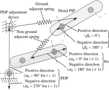
In conclusion, the installation parameters are separated into three types on the basis of their balancing objectives and position. For the ground-adjacent spring, the ground- attached installation parameter A1k is a PDP, and the link-attached installation parameter B1k is a distal PIP. For the non-ground-adjacent spring, the installation parameter Aik is a proximal PIP, and Bik is a distal PIP. The positive and negative directions of the PDPs and PIPs are determined as (90°, 270°) and (0°, 180°), respectively, as shown in Fig. 7. In addition, to enable adjustment, the PDPs must fit on PDP adjustment devices. PDP adjustment devices are used to adjust PDPs, and they can be locked at any position along the vertical axis, as shown in Fig. 7.

Positive direction (αik = 0° for i ≠ 1) Negative direction (αik = 180° for i ≠ 1)

  

Proximal PIP PDP adjustment

device

Positive direction (βik = 0°) Negative direction

(βik = 180° )

Distal PIP

 



Ground adjacent spring

Non-ground adjacent spring

Positive direction (αik = 90° for i = 1) Negative direction (αik = 270° for i = 1)

  

PDP Distal PIP

Fig. 7 Definition of the direction of PDPs and proximal and distal PIPs. Schematic of a PDP adjustment device.

(27)

Chapter 3 Determination PDP and PIP arrangements

3.1 Arrangement of PDPs

According to Section 2.2, only ground-adjacent springs contain PDPs. In this section, the characteristics of PDPs are obtained by analyzing the equations of the first row of the total SBM [Tuv]. To increase the efficiency of the adjustment, PDPs should be linear to the change of payload. For a set of balancing equations with linear solutions, the number of unknowns must be equal to the number of subsets of equations. To enable PDPs A1k to be adjustable for various payloads mp, A1k is determined to be unknown for the simultaneous equations of the entries in the first row.

In the balancing equations of the first row component matrices of Tuv, there are (n – 1) component matrices T12 to T1n. Therefore, (n – 1) equations are in the first row. For each fitted spring S1k, one distinct unknown of PDP A1k is added to the system. A total of (n – 1) springs should be connected on link 1; therefore, the total component matrices T1v

(for v = 2, …, n) can be rearranged as

 



























   









^ ^

 gm W k A B v n

n v

A k B

A k W gm

n n n n p

n

v j

j j v

v v v n p

k k v v

v

0

1 ..., , 2 0

1 1 1

1 1 1 1

1 1

2 1 1 1

1

I

I K

G

T (22)

(28)

All component matrices in Eq. (22) have the same orientation. Consequently, subset equations can be solved regardless of the orientation. The subset equations have the form of a first-order linear system. Therefore, Eq. (22) can be expressed as the matrix form of a linear system.











































n p p p

n n n

n n n v

W gm

A A A

B k

k k k

B k

k k

k B

k



















3 2

1 13 12

1 1

1 1 14

13 13

1 1

13 12

12

0 0

0

(23)

The solutions of PDP A1k (for k = 2, …, n) can be arranged as a subset of the linear equations of payloads, which can be expressed as

n ..., , k for D m C

A₁_k  _k _p  _k 2 (24)

where Ck is the coefficient of the payload, which represents the displacement of the PDP according to the payload, and Dk is the constant of the PDP, which represents the initial position of PDPs. In addition, Dk is determined by the constants of PDPs succeeding it.

Ck and Dk can be expressed as



 

 











 



 ⁿ

k

j j

k k

k for k n

B B

k C g

1 1

..., , 1 2

1 (25a)











 







 















1 ..., , 1 2

1

1 1 1

1 1

n k

D k B W

k

n k B W

D k _n

k j

j j k

k k

n n n

k (25b)

(29)

According to Eqs. (25a–b), the PDPs are separated into two sets. The preceding set is used to balance the gravitational potential energy of various payloads mp. The latter set is used to balance the constant gravitational potential energy of the links. In conclusion, the configuration of ground-adjacent springs has the following characteristic.

CH1: For an n-link VPM, (n – 1) PDPs are used to compensate for the variations in

the potential energies owing to changes in the payload. These PDPs are linear functions of the payload and can be formed by installing (n – 1) ground-adjacent springs; that is, S1k (for k = 2, … , n) of an n × n spring configuration matrix is nonzero.

3.2 Arrangement of PIPs

The spring embedded between the ground and the end link produces nonzero terms in all components of the elastic SBM. However, only the terms in the first row are used to compensate for the gravitational potential energies; the other terms are excess elastic potential energies that are compensated by non-ground-adjacent springs.

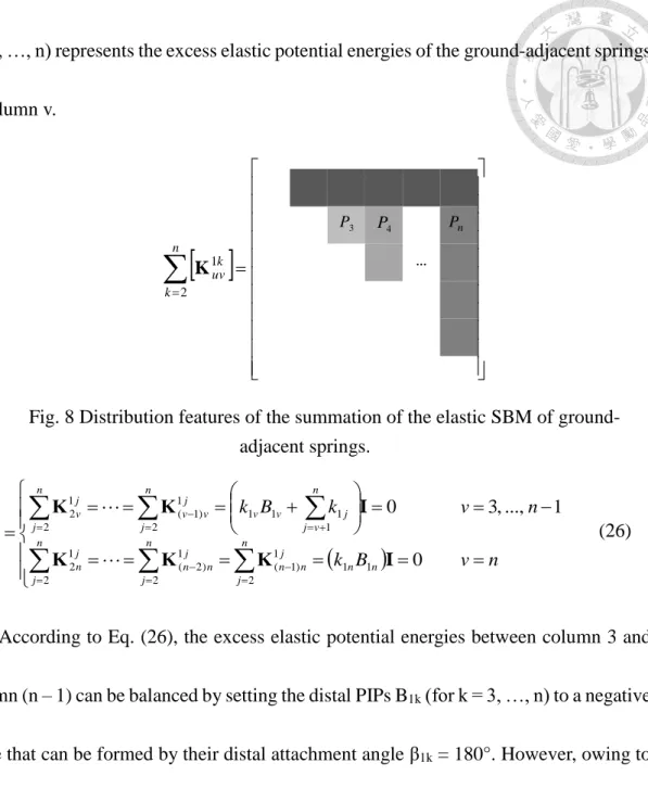
Before installing non-ground-adjacent springs, it is necessary to identify the distribution of excess elastic potential energies in their elastic SBM. According to CH1, ground-adjacent springs S12 to S1n are installed, and the sum of their non-first-row elastic SBM has the same equations in the same column, as shown in Fig. 8 and Eq. (26). P (for

(30)

v = 3, …, n) represents the excess elastic potential energies of the ground-adjacent springs in column v.

 

…





















 n

k k uv 2

K1

P3 P₄ Pn

Fig. 8 Distribution features of the summation of the elastic SBM of ground- adjacent springs.

 

















 







 



  



 







 



n v B

k

n v

k B

k

n

j

n n j

n n n

j j

n n n

j j n

n

v j

j v

v n

j j

v v n

j j v v

2

1 1 1

) 1 ( 2

1 ) 2 ( 2

1 2

1 1 1

1 2

1 ) 1 ( 2

1 2

0

1 ..., , 3 0

Κ I Κ

Κ

Κ I Κ

P



(26)

According to Eq. (26), the excess elastic potential energies between column 3 and column (n – 1) can be balanced by setting the distal PIPs B1k (for k = 3, …, n) to a negative value that can be formed by their distal attachment angle β1k = 180°. However, owing to the constraint that B1n cannot equal zero, spring S2n must be installed to compensate for the excess elastic potential energies in column n. Therefore, the installation of spring S2n

entails the following characteristic.

(31)

CH2: For an n-link VPM, a spring must be connected between link 2 and link n to

compensate for the excess potential energies between link n and the links preceding it; that is, S2n of an n × n spring configuration matrix must be non-zero.

Therefore, after the installation of spring S2n, the final column of the non-first-row total SBM can be rearranged as

 





















 

1 ..., , 3 0

2 0

2 2 1 1 2

2

2 2 2 1 1 2

2 2

n u

B k B k B

k

u B

A k B k B

A k

n n n n n

n n

n n n n n n

n n n

un P I I

I I

T P (27)

If the distal PIP B1q (where q denotes a number between 3 and n) is set as a positive value (i.e., distal attachment angle β1q = 0°), spring S2q must be installed, and its distal PIP B2q must be set to a negative value (i.e., distal attachment angle β2q = 180°) to compensate for the excess elastic potential energy. Therefore, the distal PIP of springs S1q

and S2q (for 3 ≤ q ≤ n) has the following characteristic.

CH3: For an n-link VPM, if the distal PIP of S1q is not attached in the negative direction of link q, a spring with a distal PIP attached in the negative direction is required to fit between links 2 and q (where q denotes a number between 3 and n).

Therefore, without the installation of spring S2q, column q of the non-first-row total SBM can be rearranged as

(32)

n q and q

u k

k B

k

N

q j

j n

q j

j q

q

uq      





  



 









3

; 1 ..., , 2 0

1 2 1

1 1

1 I

T (28)

Otherwise, with the installation of spring S2q, column q of the non-first-row total SBM can be rearranged as

















 



 



   





 







   



 



















n q and q

u B

k k k

B k

n q and u

B A k A k k

B k

N

q j

q q j n

q j

j q

q

N

q j

q q q j j n

q j

j q

q

uq

4

; 1 ..., , 3 0

3

; 2 0

1

2 2 2 1

1 1

1

2 2 2 2 2 1

1 1

1

I I

T (29)

where N denotes the spring that have been installed between link 2 and the links succeeding link q. For example, if springs S24 and S26 are installed, N = 4 and 6 should be considered in the balancing equations of T23.

According to Eqs. (27) and (29), after the installation of the springs connected between link 2 and the links succeeding link 2, the balancing equation in row 2 is different from those in the other rows. To solve the sequence of balancing equations without installing other springs Sik (for i ≠ 1, 2), each term in the same column should be the same

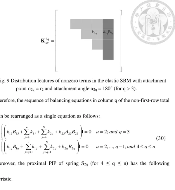
in its elastic SBM, and this can be achieved by setting its proximal PIP as A2q = –1 (i.e., position 𝑎2q = rq and attachment angle α2q = 180°). Therefore, the distribution features of

the nonzero terms are as shown in Fig. 9. Note the following exceptional case: when the elastic SBM of spring S23 is fitted in one field, it corresponds to one balancing equation only. Consequently, its proximal PIP A23 can be set at an arbitrary position.

(33)



















q uv

K2

k₂q k₂_qB₂_q

Fig. 9 Distribution features of nonzero terms in the elastic SBM with attachment point ɑ2q = r2 and attachment angle α2q = 180° (for q > 3).

Therefore, the sequence of balancing equations in column q of the non-first-row total SBM can be rearranged as a single equation as follows:

















 



 



   



 



 



   













n q and q

u B

k k k

B k

q and u

B A k k k

B k

N

q j

q q j n

q j

j q

q

N

j j n

j j

uq

4

; 1 ..., , 2 0

3

; 2 0

1

2 2 2 1

1 1

1

4

23 23 23 2 4

1 13

13

I I

T (30)

Moreover, the proximal PIP of spring S2q (for 4 ≤ q ≤ n) has the following characteristic.

CH4: For an n-link VPM, the proximal PIP of S2q must be attached to joint 1 to compensate for the excess elastic potential energy without fitting non-ground- and non-link-2 adjacent springs; that is, Sik (for i, k ≠ 1, 2) of an n × n spring configuration matrix must be zero.

3.3 Admissible spring configuration matrices for different DOF VPM

According to CH1–4, the spring configurations that can be applied for the VPM are

(34)



















) 2 , 1 , ( 0

) , 2 (

#

) 1 ..., , 3 , 2 (

0

#

) ..., , 2 , 1 (

#

k i for

n k i for

n k

i for or

n k

i for

S_ik (31)

Base on Eq. (31), the admissible spring configurations of 2-, 3-, and 4-DOF VPMs are derived and shown in Table 1 (2-A), (3-A), (3-B), (4-A), (4-B), (4-C), and (4-D).

For a general arrangement with general displacement (i.e., the coefficients of PDPs are different), the number of required PDP adjustment devices is equal to the number of ground-adjacent springs, which is expressed as

1

 n

N_p (32)

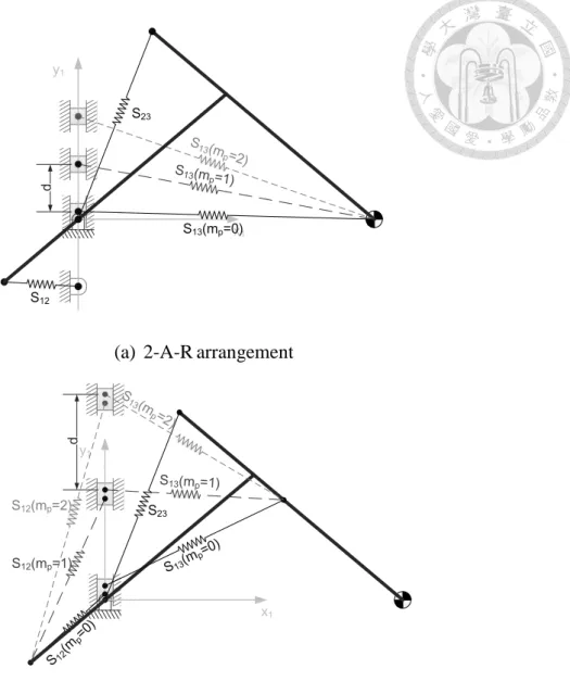
3.4 Demonstration of 2, 3-DOF VPM

An example of a 2-DOF VPM with three springs is derived. The spring configuration matrix contributed by five springs is denoted as (2-A) in Table 1. The balancing equations of the off-diagonal upper triangular total SBM can be derived accordingly. T12, T13 are the balancing equations of the gravitational and elastic potential energies, and T23 is the

excess potential energies.

13 0

13 12 12 12 2

12 W gm_p k A B k A 

T (33a)

13 0

13 13 3

13 W gm_p k A B 

T (33b)

and

23 0

23 23 13 13

23 k B k A B 

T (33c)

具有線性及接地調整方式之可變負重之靜平衡鉸接式平面操作器之設計

國立臺灣大學工學院機械工程學系 碩士論文

Department of Mechanical Engineering College of Engineering

National Taiwan University Master Thesis

具有線性及接地調整方式之可變負重之靜平衡

鉸接式平面操作器之設計

Design of Planar Various-Payload Balanced Articulated Manipulators with Actuated Linear Ground-Adjacent

Adjustment

蔣瑋軒

Wei-Hsuan Chiang

指導教授：陳達仁 博士 Advisor: Dar-Zen Chen, Ph.D.

中華民國 105 年 7 月

中文摘要

ABSTRACT

Table of contents

List of Tables

List of Figures

Chapter 1 Introduction

Chapter 2

Characteristics of SBM



 





   



 

 





   

 

 

  

 

 

 

 

 











 









 

  

 



  

Chapter 3

Determination PDP and PIP arrangements

 









 



 

  







 

 

 

 













國立臺灣大學工學院機械工程學系碩士論文

指導教授：陳達仁博士 Advisor: Dar-Zen Chen, Ph.D.