行政院國家科學委員會專題研究計畫 期中進度報告
智慧型人形機器人的發展(2/3)
期中進度報告(精簡版)
計 畫 類 別 : 個別型 計 畫 編 號 : NSC 95-2221-E-002-236- 執 行 期 間 : 95 年 08 月 01 日至 96 年 07 月 31 日 執 行 單 位 : 國立臺灣大學機械工程學系暨研究所 計 畫 主 持 人 : 黃漢邦 處 理 方 式 : 本計畫可公開查詢中 華 民 國 96 年 07 月 11 日
1
行政院國家科學委員會專題研究計畫年度報告
智慧型人形機器人發展(2/3)
(
Development of An Intelligent Humanoid Robot)
計畫編號:NSC 95-2221-E-002-236-95C1048 執行期限:95 年 8 月 1 日至 96 年 7 月 31 日 主持人:黃漢邦 台灣大學機械工程學系 Email: [email protected] 研究人員:嚴舉樓、林俊廷、張景富、顏孝杰、鍾書耘一、中文摘要
本計畫所要開發的『智慧型人形機器人』 目標在發展一個類人形的智慧型機器人系 統,並期望能夠建構出完善的智慧型人形機 器人平台。 第二年的主要目標在建立智慧型視覺系 統,利用視覺的資訊進行三維環境重建與人 臉辨識追蹤,同時結合所發展的 RRTs- based 路徑規劃理論,規劃出人形機器人的步伐軌 跡。 此外在機構設計部分,基於第一年度的 機構設計經驗,改良第一代的人形機器人機 構 設 計 , 進 而 發 展 出 第 二 代 人 形 機 器 人 NTUHRII。 關鍵詞:人形機器人、路徑規劃、立體視覺Abstract
The main purpose of this project is to develop the complete intelligent humanoid robot platform system.
The focus of the second year is to construct a reliable, intelligent vision system which includes 3D environment reconstruction, face recognition and tracking. Moreover, a new path planning algorithm based on RRTs (Rapidly-Exploring Random Trees) framework is also proposed to generate the humanoid robot footstep planning.
On the other hand, to realize the more compact and smooth motion performance, a new generation humanoid robot platform is
developed which is the modification of first generation.
Keywords: humanoid robot, path planning,
stereo vision
二、計畫緣由及目的
In recent years, the needs of robots are increasing with the development of robots. Lots of researchers and engineers have devoted to constructing different kinds of robots, especially mobile robot. Moreover, most researchers agree that biped robot has better mobility in rough terrain.
To work, cooperate, assist, and interact with human, the new generation of robots must have anthropoid structure that accommodate the interaction with human and adequately fit in the unstructured and sizable environment. Hence, an intelligent humanoid robot which can assist and interact with human is proposed in this project.
三、研究方法
1 Path Planning
Path planning is a field of finding a path for a robot to move from one physical arrangement, a configuration, tothe desired configuration. A path planning problem can be solved using well-known search strategies if it can be mapped to a search problem. This is achieved by first constructing the configuration space.
A configuration is defined as a specific arrangement of all degrees of freedom of the
2
robot. A space C of these configurations, the configuration space (C-space), can be defined, in which every dimension represents one degree of freedom of the robot’s motion. By transforming the motion planning problem of a robot into planning the motion of a point in the configuration space, constraints due to obstacles or joint limits can be more clearly expressed. In a configuration space C, path planning can then be defined as searching for a continuous line connecting the starting configuration q and the i
goal configuration q without touching the g
obstacles C . obs
Construction of the configuration space, however, is often not a trivial process, the hardest part being mapping the obstacles into the configuration space. For multi-body articulated robots moving in a space with obstacles this can be very complicated.
For a biped robot the number of dimensions of the configuration space can easily exceed 10. Building and searching in such a configuration space can be very inefficient.
A much more efficient alternative is to plan only the footsteps and not the motion of individual joints in the robot’s legs. This effectively reduces the configuration space into two dimensions. To do this, the range of valid motion from any configuration is first calculated with forward kinematics. But still, enumerating the set of possible motion exhaustively with an optimal search algorithm such as A* can be too much of a waste. To find a path efficiently we use the Rapidly-Exploring Random Tree (RRT) [14] instead.
Rapidly-Exploring Random Trees (RRTs)
In recent years, RRT planners have been very popular for a wide variety of problems due to their ability to explore the state space efficiently. It is attractive to us in that it can adapt to any kinds of robot models, that various techniques have been developed to improve its performance, and that it can be biased using heuristics designed for a specific problem to obtain a path with desired characteristics. We
will now introduce the basic RRT planner and how we fit our problem into it.
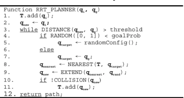
The algorithm of a basic RRT planner is shown in Table 1. For any implementation, three functions need to be provided: DISTANCE(), EXTEND(), and COLLISION(). The main differences in many RRT-based planners often lie in these functions.
Table 1 Basic RRT planner
Function RRT_PLANNER(qi, qg) 1. T.add(qi);
2. qnew ← qi;
3. while DISTANCE(qnew, qg) > threshold 4. if RANDOM([0, 1]) < goalProb 5. qtarget ← randomConfig(); 6. else
7. qtarget ← qg;
8. qnearest ← NEAREST(T, qtarget);
9. qnew ← EXTEND(qnearest, qrand);
10. if !COLLISION(qnew)
11. T.add(qnew);
12. return path;
The function DISTANCE() returns the distance between two configurations. In an RRT planner, this information is in turn used to find the nearest node to another node. Often, the function means more than the Euclidean distance between the states two configurations represent. Instead it is more similar to a heuristic function as in heuristic search. And indeed, with goal probability set to one the RRT planner reduces to A*.
EXTEND() returns a new configuration reachable from the configuration stored in an existing search node. As determined by each variant of RRT planner this new configuration may be the best one calculated analytically, or drawn from a set of controls.
COLLISION() normally determines if a configuration collides with the map. This is done by mapping the robot configuration to the state space.
The growth of an RRT can be affected via
biasing, that is, by directing the growth to
configurations other than the randomly chosen ones for some probability. The most commonly used one is the goal bias shown in line 7 in Table 1.
3
Planning Under Kinematic Constraints
RRT is an ideal tool for path planning with kinematic constraints, since its tree structure readily accommodates possible set of control inputs at each configuration. In this regard, search on grid space and most potential field methods are not applicable. However, planning with kinematic constraints has its own issues to solve, which we will discuss in this section.
The original variant of RRT does not care about kinematic constraints. In the C-space of a holonomic system, a configuration can freely connect to other configurations in any directions. For these systems, a node q can simply extend
toward the direction of the target configuration
target
q for some set distance to obtain a new configuration qnew. For planning the footsteps of
a biped robot, however, the available controls do not map to directions of motion directly. Fortunately this is not hard to remedy.
A common approach is to discretize control input into a set of possible controls, denoted U, which constitute possible branches of each search node in the RRT. The extension algorithm is given in Table 2. At each extension of the tree, the nearest node to the chosen configuration is first found out, and then all of its possible controls are evaluated. The resulting one closest to the target will be kept as a new node in the tree, thus giving a way to obtain qnew in
nonholonomic planning.
Table 2 RRT-Extend with discrete controls
Function EXTEND(q, qtarget) 1. qnew ← null; 2. dmin ← ∞ 3. for each u in U 4. apply u to obtain qu 5. if COLLISION(qu) 6. continue;
7. if dmin > DISTANCE(qtarget, qu)
8. qnew ← qu
9. dmin ← DISTANCE(qtarget, qu)
10. return qnew;
Discretizing controls can let an RRT-based planner “backtrack” – that is, to seek alternative choices when the seemingly best sub-tree cannot lead to solution. If an extension from a node
using a specific control has failed, this failure can be “memoized” to prevent further attempts. This backtracking mechanism is present in all common graph search algorithms, but has been largely ignored in RRT planners. This is a significant weakness of the original form of RRT planner in constrained environments, where unsuccessful edge extensions can be attempted repeatedly.
It is also worth noting that, discretizing controls effectively turns the planning problem into a graph search problem, reducing the completeness of the planner to the resolution of the discretization. This is rarely a problem though unless in very challenging environments, given sufficient resolution. And there is usually much more to gain in performance than to lose in completeness. In all works we have seen it seems that this set of controls is chosen arbitrarily or empirically.
For starters, we choose the set of controls: { 2.0, 0 , 1.4, , 1.4, }
6 6
π π
= −
U , in which
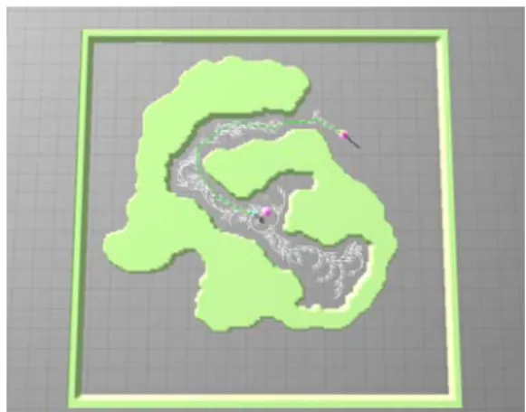
each control consists of a pair of forward displacement in meters and rotation in radians. A path for our biped robot planned using RRT with this control set is shown in Figure 1.
Figure 1 A path planned with RRT
Distance Metric
The RRT uses the function DISTANCE() to determine which node is the nearest one to a target configuration. To do this the notion of “distance” must be defined.
4
L1 metric, which indicates the Manhattan distance, and the L2 metric, which indicates the Euclidean distance, between the positions two configurations represent. In grid space the L1 metric is most convenient, and in other cases the L2 metric is the most intuitive. A distance metric can also be defined in the configuration space without modification to search algorithms provided that it is consistent.
We used the L2 metric in pervious experiments. However, while being straight-forward and always consistent, L2 metric is not good enough when the robot kinematics is nonholonomic, e.g., when planning for our biped robot as shown in Figure 2. A position right at the side of the robot can take much more time to reach than a position in front, making the L2 metric a wrong indication of distance between nodes. If the L2 metric is used in these scenarios suboptimal nodes will be chosen for expansion, leading to higher computation cost.
Figure 2 L2 metric is not good for biped robots
Better Distance Metric
An RRT planner is most commonly biased toward the goal configuration. In that case, the node chosen for expansion is the one with the least distance to the goal, as determined by the distance metric, of which the most commonly used is the L2 metric.
For holonomic robots in simple environments this works well, but as the robot kinematics and the environment get more complex its performance degrades significantly. This is partly because the L2 distance to the goal is no longer a good indication of the cost to reach the goal in those situations. Some extreme examples can be found in [15]. As LaValle
concludes an environment can always be designed to make an RRT planner perform very poorly, such as nesting or cascading multiple bug traps. Even though a path when exists is guaranteed to be found eventually with RRT, in some situations the higher computation cost can make a difference between finding a solution or not if deliberation time is limited.
For our problem we have found a simple yet effective way to bias an RRT planner. This idea combines the venerable navigation function (NF) [11] as a distance metric with the RRT.
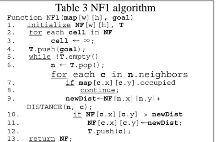
Navigation functions are a special kind of potential fields which do not suffer from local minima. The simplest and arguably most widely used navigation function is the ones built in grid space using the NF1 wave front propagation algorithm, shown in Table 3:
Table 3 NF1 algorithm
Function NF1(map[w][h], goal) 1. initialize NF[w][h], T 2. for each cell in NF 3. cell ← ∞; 4. T.push(goal); 5. while !T.empty() 6. n ← T.pop();
for each c in n.neighbors
7. if map[c.x][c.y].occupied 8. continue; 9. newDist←NF[n.x][n.y]+ DISTANCE(n, c); 10. if NF[c.x][c.y] > newDist 11. NF[c.x][c.y]←newDist; 12. T.push(c); 13. return NF;
An example navigation function is shown in Figure 3. The resulting potential function only has one local minimum: the global minimum at the goal configuration. This method is useful in that it preserves the simplicity of the potential field method while giving resolution-optimal directions of motion to the goal at every position in the map.
As planning starts, a navigation function toward the goal can be built to provide motion directions optimal up to the navigation function resolution at any place in the map. If the gradient of the underlying navigation function is used for biasing towards the goal, it would always be the optimal bias regardless of the complexity of the static part of the environment, only that it does not take kinematic constraints of the robot into
5
account.
Also, because the navigation function only needs to be built once before the robot reaches its destination, there is almost no overhead computationally by using the gradient of navigation function as the bias towards the goal. A benchmark using the environment in Figure 4 is carried out for 500 runs, and performance of RRT using L2 metric and the improved distance metric are shown in Figure 5. Enormous performance gain is obtained with the improved distance metric.
Figure 3 An indoor map (top), and the navigation function built with NF1 (bottom)
Figure 4 Environment with deep local minima
0 1 2 3 4
L2
NF
Figure 5 Boxplot of planning time (in seconds) for RRT with L2 and NF distance metric
2. Humanoid Footstep Planning
After producing the 2D trajectory by the method we mentioned above, the humanoid robot step trajectory can be generated easily. The footstep trajectory generation procedure is listed below.
1. DefineLmax,1 and Lmax,2 as the upper bound
and lower bound of the acceptable step distance, respectively.
2. Defineθmax,1 θmax,2 as the upper bound and
lower bound of the acceptable angle change in one step.
3. Choose the first input knot point planned for the robot as the reference point.
4. Choose the next point of the reference point as the compared point.
5. Compute the distance and the change of the direction between the reference point and the compared point. If the distance or angle doesn’t exceed the limit values, choose the next point of the input trajectory as compared point.
6. Iterate the step 5 till either the distance or angle exceeds the Lmax,1 or theθmax,1.
7. If the computed value in step 6 (distance or change of angle) falls betweenLmax,1 and
max,2
L or θmax,1 and θmax,2 , choose the current compared point as new reference point.
8. If the computed value in step 6 exceeds
max,2
L or θmax,2, interpolate a new point that makes the computed value equals to Lmax,1
or θmax,1, and set it as new reference point. 9. Collect all the reference points and find all
6
collected points.
10. Define the distance between two legs as W. The position of each foot trajectory falls on the direction of the corresponding tangent vector with W/2 displacement from the corresponding reference point.
11. The direction of the foot pad of each foot trajectory is parallel to the corresponding normal vector.
12. With the procedures above, we can plan the foot trajectory as Figure 6.
Figure 6 The planned steps of biped robot
3. Stereo Vision
The human visual ability to perceive depth is both commonplace and puzzling. We perceive three-dimensional spatial relationships effortlessly, but the means by which we do so are largely hidden from introspection. One method for depth perception that is relatively well understood is binocular stereopsis, in which two images recorded from different perspectives are used. Stereo allows us to recover information about the three-dimensional location of objects-information that is not contained in any single image. A considerable amount of research has been directed toward finding computational models for stereo vision and for related human perceptual abilities[1][17][18].
Stereo is an attractive source of information for machine perception because it leads to direct range measurements, and, unlike monocular approaches, does not merely infer depth or
orientation through the use of photometric and statistical assumptions. Once the stereo images are brought into point-to-point correspondence, recovering range values is relatively straightforward. Another advantage is that stereo is a passive method. Although active ranging methods that use structured light [19], laser range finders, or other active sensing techniques are useful in tightly controlled domains, such as industrial automation applications, they are clearly unsuitable for more general machine vision problems.
Three applications have received the most attention:the interpretation of aerial photographs for automated cartography, guidance and obstacle avoidance for autonomous vehicle control [2][22], and the modeling of human stereo vision [17][18]. Other applications include industrial automation, and the interpretation of microstereophotographs [8] for biomedical applications. Each domain has different requirements that affect the design of a complete stereo system.
The main goal is aimed to construct a stereo vision system for depth estimation. Two commercial USB webcams are used to acquire stereo image pairs instead of using expensive instruments. Through stereo matching process, the correspondence can be easily found, thus the disparity can be surely determined. After disparity estimation and post-process, depth information can be obtained by stereo triangulation.
Figure 7 shows the flow chart of the stereo vision system. At first, camera configuration must be check to make sure of the epipolar constraint. Although the webcams are coaxial configured to approximately coplanar geometry, there is still slight vertical offset that can not be detected by visually check. Therefore, camera rectification is a necessary step before stereo matching. In addition to camera rectification, stereo camera calibration is another necessary step. Parameters estimated by camera calibration are needed for stereo triangulation and increasing the accuracy of the range estimation. When the camera configuration is confirmed, stereo matching and stereo triangulation are performed
7
after.
The stereo matching procedure is shown schematically in Figure 8. At first, color space is transformed from RGB color model to YCC color model. Multilevel images are then constructed for winner-update strategy. Epipolar lines are aligned to simplify the search range from two-dimension to one-dimension. Matching is driven from left to right and the candidates are selected by using winner-update strategy. During the matching process, ordering constraint, photometric constraint, chromatic constraint and uniqueness assumption are added to reduce the ambiguities and make the matching results more accurate. The determination of correspondence is selected by using a proposed criterion called the color weighted correspondence algorithm and the W.T.A. (Winner-Takes-All) method. After the matching process, left-right checking is used to validate the consistency and detect occlusion. Areas that left-right checking fails are labeled as occlusion. The disparities of occlusion areas are always incorrect, so interpolation process must be done in these areas. Finally, a dense disparity map can be obtained.
The stereo vision system is composed of one PC and two commercial USB webcams. The framework of the system is shown in Figure 9. The webcams are coaxial configured to approximately coplanar geometry as show in Figure 10.
To simplify the search range from two-dimension to one-dimension due to epipolar constraint, the webcams are coaxial configured to approximately coplanar geometry beforehand. In order to make sure the webcams are parallel, projected median is adopted to rectify slight vertical offset that not visually obvious. Before performing stereo matching, camera rectification through block matching is used to estimate the slight vertical offset, as shown in Figure 11. In order to search the vertical offset, the search range is two-dimension.
Figure 7 Flow chart of the stereo vision system
8
Figure 9 System Description
Figure 10 Webcam configuration
Figure 11 Camera rectification through block matching
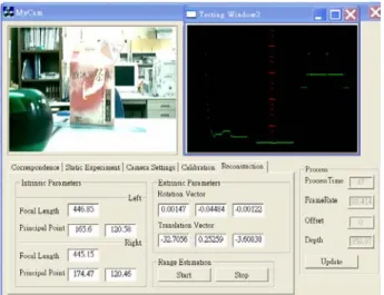
A carton is used to test the depth estimation, as shown in Figure 12. We use the middle row in image .to estimate the depth information. Due to the disparity constraint, search range of the system is about 60 pixels. In order to enhance the reliability, we use support window size=32 32× ,
10
γ = . The image size is 320 240× . Table 1 shows the disparity versus depth chart. The pink line represents the depth computed by system. The blue line represents the depth calculated.
The calculation error is caused by floating point error. We can see that the error becomes enormous when the disparity getting smaller. The system yields an accurate depth estimation resolution (5 mm) from 30 to 60 cm. From 60 to 150cm, the resolution becomes about 5 cm.
In order to construct a near real-time stereo vision system for depth estimation and 3D reconstruction, a complete and practical procedure is constructed to reach the goal. It can be divided into two main tasks. One is camera configuration, and the other is stereo matching methodology.
Figure 12 Carton in the left window is used for depth estimation
Table 4 Disparity versus depth chart
0 200 400 600 800 1000 1200 1400 1600 1800 21 23 25 27 29 31 33 35 37 39 41 43 45 47 49 51 53 55 57 59 Disparty (pixels) D ep th ( mm) Theoretical depth True depth
Cameras must be rectified before performing the stereo matching in case mismatches happen. Projected median is used to achieve this goal. It performs well as the cameras are set up in approximately correct position. After camera rectification, camera calibration is a necessary procedure for accurate depth
9
estimation and 3D reconstruction. In particular, it is a critical task for stereovision analysis. Each camera is calibrated independently and then applying geometric transformation of the external parameters to find out the geometry of the stereo setting.
The YCC color model is adopted to simulate human vision system to deal with textureless regions. It is then applied to the correspondence determination. The proposed “color weighted correspondence algorithm” is used to fast determine the correspondence. Experimental results show the idea of color weight is practicable and reasonable for stereo matching tasks. Some geometric constraints are included to reduce ambiguities. A mechanism called left-right checking is used to find occlusion. After post-processing, a smooth dense disparity map can be obtained. Thus, the three-dimensional characteristics of objects can be recovered and utilized to do upper level tasks, such as navigation, simultaneous localization and mapping, and intelligence traffic system. Finally, a 3D-display monitoring system is constructed for displaying the 3D reconstruction results.
The experiments obtain successful depth information and 3D image reconstruction results. It validates the feasibility of humanoid color perception with stereo matching methodology to estimate depth and reconstruct 3D scene. It makes the system like the human vision system more.
4. Multi-View Faces Tracking and Recognition
We propose a novel method (Multi-CAMSHIFT), which is based on the characteristics of color and shape probability distribution, to solve the tracking problems for multiple objects. The tracker is used to get the candidate regions by outlining the interested probability distribution. The system performance is further improved by using multi-resolution framework. The principal component analysis (PCA) and support vector machine (SVM) are integrated to form the multi-view faces detection
and recognition module for classifying different face poses and identities. Beside color information, the gray background image is used to locate the human head in the region of tracking pedestrian based on probability distribution rule. The rule can also be used for skin color face tracking to remove background region (non-face region). Since the proposed Multi-CAMSHIFT (MCAMSHIFT) is computationally efficient, it can work in complex background and track in real-time. The slowly changing lighting condition is effectively resolved using probability model update. From experiments, the proposed MCAMSHIFT was successfully applied to multi-view faces tracking and recognition. It can also be applied to surveillance system, pedestrian tracking and face guard systems.
Interested Probability Modeling
Interested probability plays an important role in CAMSHIFT algorithm because the convergence size of search window is based on it. For tracking objects, the characteristics of target which we are interested in can be chosen to construct interested probability model. In the tracking system, two methods are proposed to achieve.
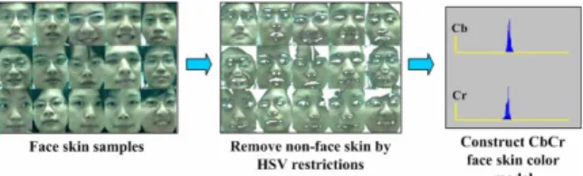
(a) Skin Color Probability Modeling
Skin-color is only clustered in a small area in color space. Human color appearances differ more in brightness than in chroma, and the difference between colors is mainly caused by intensity of the color itself; under a certain lighting condition, skin-color distribution can be approximated by Gaussian Model in normalized color space. The main advantage of converting the image to the YCbCr domain is that influence of luminosity can be removed during our image processing. In the RGB domain, each component of the picture has different brightness. However, all information about the brightness is given by the Y-component, since the Cb and Cr components are independent of the luminosity.
As using real cameras with discrete pixel values, a problem will occur because of using HSV space. When brightness is low (V near 0),
10
saturation is also low (S near 0). Hue then becomes quite noisy, since in such a small hexcone, the small number of discrete hue pixels cannot adequately represent slight changes in RGB. This then leads to wild swings in hue values. To overcome this problem, we simply ignore hue pixels that have very low corresponding brightness values. With sunlight, bright white colors can take on a flesh hue so we use an upper threshold to ignore flesh hue pixels with corresponding high brightness. At very low saturation, hue is not defined so we ignore hue pixels that have very low corresponding saturation [3]. The restrictions of HSV color space are used to remove most non-skin color regions in face skin samples. We can construct the skin probability CbCr model by removing non-skin region from the face skin samples Figure 13 shows the results.
Figure 13 Construct face skin color model
(b) Background Probability Modeling
We obtain the initial background parameters from a short video sequence without any moving objects. The median value of intensity at each pixel location in all images is determined as the value of intensity at the corresponding pixel location in the initial background model. This process is called background subtraction, and scene representation is called the background model. Pixel intensity is the most commonly used feature in background modeling. If we monitor the intensity value of a pixel over time in a completely static scene, then the pixel intensity can be reasonably modeled with a Gaussian distributionPr(x)~N(μ,σ2).
Modified CAMSHIFT Algorithm
MCAMSHIFT is based on CAMSHIFT. The procedure and concept of MCAMSHIFT are reconstructed. The most important job is to combine each CAMSHIFT. Each CAMSHIFT tracker obtains the variables, which is the
boundary restrictions of a defined region by other trackers. By verifying the variables, the defined region will not be redefined. In order to reduce unnecessary calculation, the interested probability of search window boundaries of the former search members is ignored. Therefore, each search member will not be affected by other search members and work independently. The algorithm is described below.
1) Set the initial search number.
2) Each search member ignores the interested probability in the search window of the former search members and performs the modified-CAMSHIFT process.
3) Each search member records the search window boundary of the former search members.
4) Judge which search member is divergent, and initialize the parameters of the divergent search member.
5) If any search member disappears, sort search members by the sort index method and update search number; otherwise, add search number.
6) Repeat step2.
11
The search number indicates the number of CAMSHIFT trackers, and a search member represents each CMASHIFT tracker. In the Step4, the goal of initializing the parameters of the divergent search member is to avoid the problems when new search member is created. The problems include wrong information which belongs to the former member, such as position, size and other parameters, etc.
Multi-View Faces Detection and Recognition
Color information of images has obvious attributes to segment the skin region of face candidate. However, in face detection and recognition module, the gray pattern is taken in the search window as face feature. The histogram equalization operation is used to solve lighting condition problems for gray pattern. Besides, we propose the check boundary probability distribution rule as face region mask filter to remove non-face background region. The rule can also be used to define head tracking in the pedestrian region.
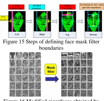
Two methods have been used to handle this problem without solving other difficult vision problems such as robust segmentation of the head shape and face skin color. This is done simply by the operator outlining the head or face of the first training set image. The background of the training set images is therefore consistently zero. Because the eigenfaces are made from a training set with the background masked from each image, they will also have values of zero at these image locations. The rule can filter non-face noise to retain only face pattern. Furthermore, the method costs a little computation time to remove noise. It can avoid the non-face noise on face region by the probability distribution of column and row. In Figure 16, eigenfaces can be modified by the rule to remove non-face region.
Steps of the checking probability
distribution rule:
1) Count interested probability of column from the farthermost side boundary.
2) Check the next column, if the probability achieve threshold, check the next column
repeatedly several times; otherwise repeat step1. 3) If several times probabilities of column achieve threshold, decide the boundary. 4) Repeat steps from1 to 3 for row and decide the top boundary according to the two side boundaries.
5) Set the bottom boundary by face ratio and the decided side boundaries.
Figure 15 Steps of defining face mask filter boundaries
Figure 16 Modified eigenfaces obtained by mask filter
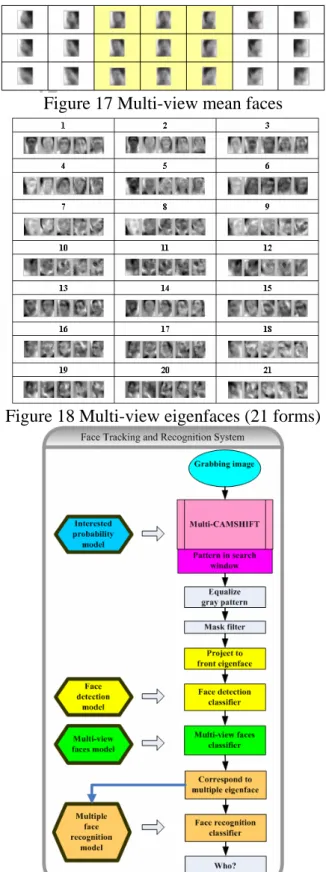
Multi-View Faces Module
In our multi-view face detection and recognition application, we combine many PCA+SVM models to extend the capability of single PCA+SVM model. Not only the face detection and recognition are considered for the front face, but also multi-view faces can be considered. To represent multi-view faces, we need multiple sets of eigenfaces and meanfaces, as shown in Figure 17 and Figure 18. So each eigenface of different poses has to be trained. The 21 forms of multi-view faces patterns (Figure 18) are used to perform the stage of the classification. The first stage is to enhance the sample by equalization and mask filter. The second one is to project the pattern to the front eigenface and implement the face detection processing. Then the face which passes the face detection classifier is checked what view the face is by multi-view faces detection procedure.
12
Finally, we can project the pattern to the corresponding eigenface and choose the corresponding face recognition model as its classifier.
Figure 17 Multi-view mean faces
Figure 18 Multi-view eigenfaces (21 forms)
Figure 19 Multiple multi-view faces tracking and recognition
Multiple Faces Tracking and Recognition
For multiple faces tracking and multi-view faces recognition system, the system is composed of four main parts; object tracking, face detection, multi-view face classification and multi-view faces recognition. The four models are constructed for those capabilities. Figure 19 indicates the flow chart of all face system.
Figure 20 indicates the multi-view faces. The system can know who he is and understand which pose of face is. And the figure shows that the system can work well no matter how the environment is simple or complex.
Figure 20 Multi-view faces tracking and recognition
5. The New Generation Humanoid Robot
We have improved the mechanism of the NTUHR-I and designed the NTUHR-II. The main modifications are listed below.
a. The distance between hip and knee should be similar to the distance between knee and ankle. Because hip-knee distance of NTUHR-I is too long to achieve certain configurations, we modify the hip-knee distance and the knee-ankle distance in NTUHR-II.
b. To reduce the torque requirement in hip, knee and ankle, the three pitch joints are aligned in a line for NTUHR-II.
c. Large knee rotation range. A special knee shape is created to allow NTUHR-II to rotate its knee joint for larger range.
d. Selection of material. Since the stiffness of aluminum is poor, partial frame of NTUHR-I sometimes bended and distorted. To increase the stiffness of mechanism, the aluminum alloy is adopted instead.
e. More difference of NTUHR-I and NTUHR-II are described in Table 5.
13
Table 5 Specification of NTUHR-I and NTUHR-II
NTUHR-I NTUHR-II
DOFs 21 24
Height 390mm 450mm
Weight 1.5kg 1.8kg
Figure 21 NTUHR-I(left), NTUHR-II(right)
Figure 22 Pitch joint arrangement
Figure 23 New design for large knee rotation range
四、結論
In this year, an intelligent vision system is developed for the humanoid robot. The vision system can provide real time 3D environment information for robot planning further. Moreover,
the real time multi-face tracking and recognition algorithm are also proposed in this year.
On the other hand, a new path planning algorithm based on RRTs is realized for obstacle avoidance and humanoid robot footstep planning. And futher, the new generation humanoid robot NTUHR-II is constructed to improve the drawbacks of the NTUHR-I.
In the next year, we will focus on the integration of control system, mechanism system, and vision system. To realize the real autonomous robot, the SLAM (Simultaneous Localization and Mapping) system will also be developed in the next year.
五、參考文獻
[1] N. Alvertos, “A Zoom-Based Stereo Camera Model,” Proceedings of IEEE Energy and Information Technologies in the Southeast,
Vol.2, pp. 482-485, Apr. 1989.
[2] S. T. Barnard and M. A. Fischler, “Computational Stereo,” ACM Computing Surveys, Vol. 14, pp. 553-572, Dec. 1982.
[3] G. R. Bradski, “Computer Vision Face Tracking for Use in a Perceptual User Interface,” Intel Technology Journal, 2nd Quarter, 1998.
[4] B. Castaneda, J. C. Cockkburn, “Reduce Support Vector Machines Applied to Real-Time Face Tracking,” ICASSP’05, Vol. 2, pp. 673-676, 2005.
[5] P. Cheng and S. M. LaValle, “Resolution Complete Rapidly-Exploring Random Trees,” Proc. IEEE Int'l Conf. on Robotics and Automation, pp. 267–272, 2002.
[6] E. Hjelmas and B. K. Low, “Face Detection: A Survey,” Computer Vision and Image Understanding, Vol. 83(2), pp. 236-274,
2001.
[7] K. Hotta, “View-Invariant Face Detection Method Baded on Local PCA Cells,”
Proceedings of the 12th International Conference on Image Analysis and Processing, 2003.
[8] F. J. Hsiao and H. P. Huang, “3D Image Reconstruction and Analysis for Micro-manipulation Systems,” Master
14 thesis, Department of Mechanical
Engineering, National Taiwan University, 2003.
[9] C. W. Hsu and C. J. Lin, “A Comparison of Methods for Multi-Class Support Vector Machines,” IEEE Transactions on Neural Networks. Vol. 13, No. 2, pp. 415-425,
2002.
[10] C. W. Hsu, C. J. Lin and C. C. Chang, “A Practical Guide to Support Vector Classification,” Department of Computer Science and Information Engineering, National Taiwan University, Taiwan.
[11] R. A. Jarvis, “Collision-Free Trajectory Planning Using Distance Transforms,”
Transactions of the Institution of Engineers,
Australia, Mechanical Engineering, Vol. 10, No. 3, pp. 187–191, September 1985.
[12] K. Jung, K.I. Kim, T. Kurata, M. Kourogi, J. Han, “Text Scanner with Text Detection Technology on Image Sequences,” In Proc. International Conference on Pattern Recognition in Quebec City, Canada, Vol.
3, pp. 473-476, 2002.
[13] J. C. Latombe, Robot Motion Planning,
Kluwer Academic Publishers, 1991.
[14] S. M. LaValle, “Rapidly-Exploring Random Trees: A New Tool for Path Planning,” Technical Report, Computer
Science Dept., Iowa State University, Oct. 1998.
[15] S. M. LaValle, Planning Algorithms,
Cambridge Univ. Press, 2006.
[16] Y. Li, S. Gong, and H. Liddell. “Support Vector Regression and Classification Based Multi-View Face Detection and Recognition,” In Automatic Face and Gesture Recognition, IEEE International Conference on, pp. 300-305, 2000.
[17] D. Marr and T. Poggio, “A Computational Theory of Human Vision,” Proceedings of the Royal Society of London, Series B, Vol.
204, pp. 301-328, 1979.
[18] D. Marr and T. Poggio, “A Theory of Human Vision,” MIT A. P. No. 451, 1977.
[19] Y. Ming, J. Jiang and J. Ming, “Background Modeling and Subtraction Using a Local- Linear-Dependence-Based Cauchy Statistical Model,” Proceedings of the 7th Digital Image Computing:
Techniques and Applications, pp. 10-12,
2003.
[20] D. Scharstein, R. Szeliski, and R. Zabih, “High-Accuracy Stereo Depth Maps Using Structure Light,” Proceedings of IEEE Computer Society Conference on Computer Vision and Pattern Recognitio, pp. 195-202,
Jun. 2003.
[21] K. J. Yoon and I. S. Kweon, “Adaptive Support-Weight Approach for Correspondence Search,” IEEE Transactions on Pattern Analysis and Machine Intelligence, Vol. 28, No. 4, pp.
650-656, 2006.
[22] L. Zhao and C. E. Thorpe, “Stereo and Neural Network-Based Pedestrian
Detection,” Proceedings of
IEEE/IEEJ/JSAI International Conference on Intelligent Transportation Systems, pp.
298-303, Oct. 1999.