使用疊代式自我一致性運算於核磁共振逆影像重建

(1)

國立臺灣大學醫學工程學研究所碩士論文

Graduate Institute of Biomedical Engineering College of Medicine and Engineering

National Taiwan University Master Thesis

使用疊代式自我一致性運算於核磁共振逆影像重建 Iterative self-consistent magnetic resonance inverse imaging

黃琮閔

Tsung-Min Huang

指導教授：林發暄博士 Advisor: Fa-Husan Lin, Ph.D.

中華民國 101 年 8 月

August, 2012

(2)

誌謝

本論文的完成得力於 Kevin 學長的大力協助，不厭其煩的指出我研究中的缺失，且總能在我迷惘時為我解惑，使得本論文能夠更完整而嚴謹。感謝指導教授林發暄博士，老師悉心的教導使我得以 MRI 窺領域的深奧，不時的討論並指點我正確的方向，使我獲益匪淺。老師對學問的嚴謹更是我輩學習的典范。感謝朱盈樺學姐還有學弟、學妹們的幫忙讓我不用忙於外務可以專心準備口試。

最後，謹以此文獻給我摯愛的雙親，能體諒我比別人多花了一年的時間卻默默的在背後支持我。

(3)

中文摘要

核磁共振逆影像(magnetic resonance inverse imaging, InI) 利用多組核磁共振射頻線圈同步接收核磁共振影像(magnetic resonance imaging, MRI) 信號以含括全腦的視區及 100 毫秒的時間解析度。其基本原理是利用不同位置射頻線圈提供的空間敏感度重建在資料擷取中所忽略的空間編碼訊息。先前研究發現逆影像在 K 空 間 (k-space, K-InI) 比起在影像空間 (image space) 使用最小範數估計解 (minimum-norm estimate, MNE)的重建可有更高的空間解析度和對大腦活動訊號更高的靈敏度。最近的研究顯示使用多通道接受器的平行核磁共振影像在 K 空間中有一訊號的自我一致性(self-consistent property)。當運用這個特性在平行影像的重建時，可以提升重建影像的品質。根據這一特性，本研究提出運用自我一致性在

核磁共振逆影像的影像重建方法。其稱為自我一致性 K 空間逆影像(self-consistent

K-InI)以及₁範數自我一致性 K 空間逆影像(₁-self-consistent K-InI)。經由模擬，

我們發現與 K-InI 相比，self-consistent K-InI 和₁-self-consistent K-InI 可以提供更 高的空間解析度。應用self-consistent K-InI 及 ₁-self-consistent K-InI 於真人視覺

功能性核磁共振影像實驗時，這些影像重建方法可在 100 毫秒時間解析度下描繪

出大腦視覺區域的血液動力學變化。Self-consistent K-InI 與 K-InI 在偵測大腦活動訊號的 BOLD 對比靈敏度相近，但是₁-self-consistent 則比 K-InI 提高約 50%的偵 測靈敏度。我們預期self-consistent K-InI 和₁-self-consistent K-InI 可以提供高時間 和高空間解析度的大腦活動訊號來進一步了解人腦功能。

關鍵字：功能磁振造影、逆影像、視覺、磁振造影、K 空間逆影像、自我一致性

(4)

ABSTRACT

Magnetic resonance inverse imaging (InI) using multiple channel radio-frequency (RF) coil detection can achieve 100 ms temporal resolution with the whole brain coverage. InI reconstructions use the RF coil sensitivity information to reconstruct the omitted partition encoding data. Previously we proposed the k-space InI (K-InI) reconstruction to provide higher spatial resolution and higher sensitivity in detecting activated brain areas in BOLD fMRI experiment than the image domain minimum-norm estimate (MNE) InI reconstruction. Recently, the self-consistent property has been suggested as a useful property in k-space parallel MRI reconstruction because it improves the reconstruction image quality. Studying this study, we develop self-consistent K-InI and ₁-self-consistent K-InI algorithms to use the self-consistent property to reconstruct highly accelerated InI acquisitions. Numerical simulations show that self-consistent K-InI and ₁-self-consistent K-InI can provide higher spatial resolution than K-InI. Applying self-consistent K-InI and ₁-self-consistent K-InI to BOLD contrast fMRI experiments, we found that all methods can reveal visual cortex activation at the 100 ms temporal resolution. Self-consistent K-InI has a comparable detection sensitivity to K-InI. ₁-self-consistent K-InI the sensitivity of detecting brain activation is 50% higher than that of K-InI. Self-consistent K-InI and ₁-self-consistent K-InI can be useful tools in fMRI data analysis to characterize brain activity with a high spatiotemporal resolution.

Keywords: fMRI, InI, visual, MRI, K-InI, self-consistency

(5)

LIST OF FIGURES

Figure 1. The left-hand side of figure is the reference scan, and we used the center of k-space data to compose the calibration matrix A^ACS. ... 9 Figure 2. K-InI reconstruction uses the phase encoding data at the k-space center

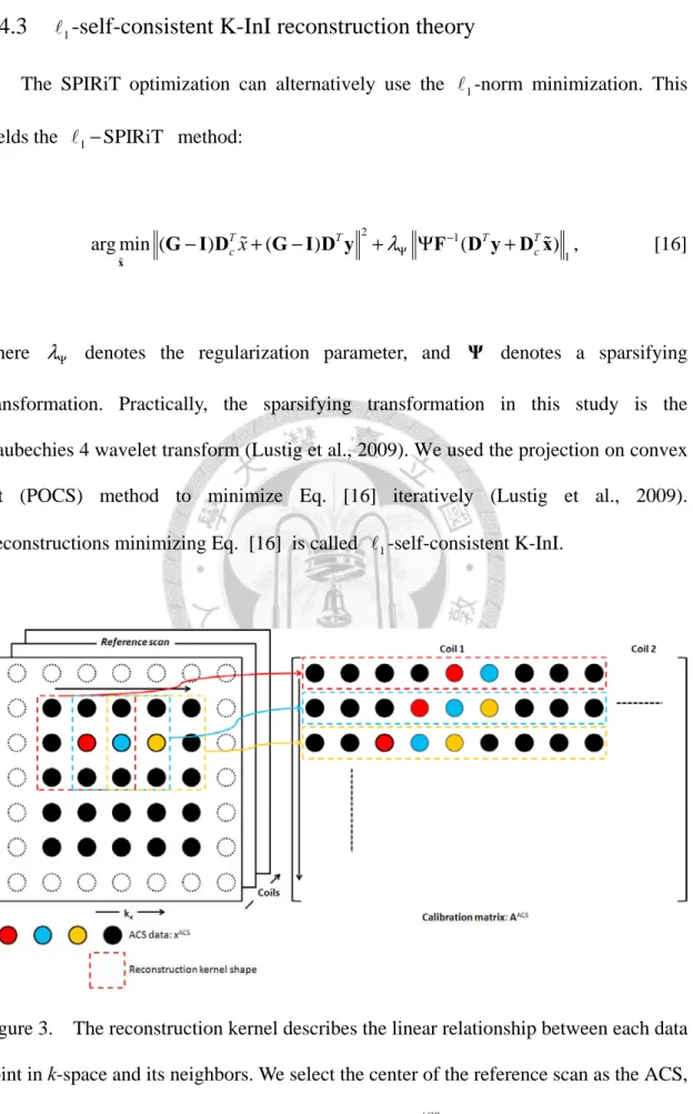
AACC to interpolate the skipped k-space data. ... 11 Figure 3. The reconstruction kernel describes the linear relationship between each data point in k-space and its neighbors. We select the center of the reference scan as the ACS, and use the ACS to construct the calibration matrix A^ACS. ... 16 Figure 4. The RMSE of the reconstructed images using K-InI, self-consistent K-InI

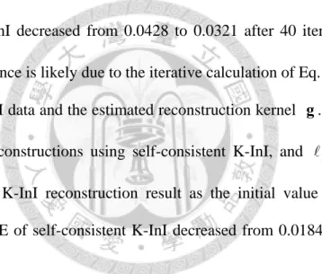
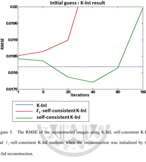
and ₁ -self-consistent K-InI methods when the reconstruction was initialized by a zero vector. ... 21 Figure 5. The RMSE of the reconstructed images using K-InI, self-consistent K-InI

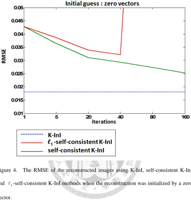
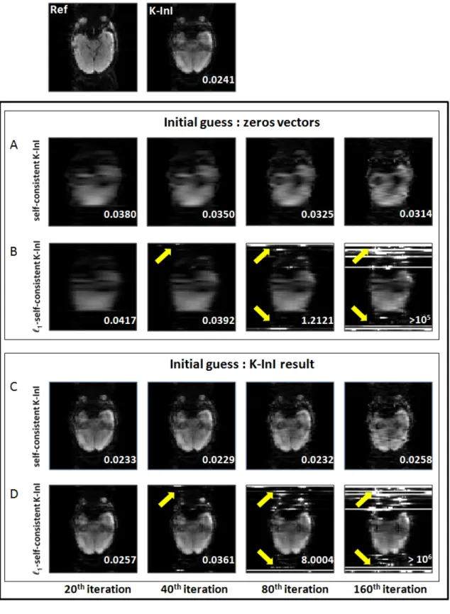
and ₁ -self-consistent K-InI methods when the reconstruction was initialized by the K-InI reconstruction. ... 22 Figure 6. The sum-of-squares reference image (SoS) and K-InI reconstruction. Panels A and B show the self-consistent K-InI and the ₁-self-consistent K-InI reconstruction after 20, 40, 80, and 160 iterations using a zero-vector as the initial value. Panels C and D show the self-consistent K-InI and the

1-self-consistent K-InI reconstruction after 20, 40, 80, and 160 iterations using K-InI reconstruction as the initial value. ... 24 Figure 7. The reconstructed visual cortex images of K-InI, self-consistent K-InI, and

1-self-consistent K-InI at different SNRs. Reconstructions were linearly scaled between 0 and 1 to illustrate the spatial distribution. The simulated

(7)

visual cortex ROI is shown as the green area. ... 26 Figure 8. The reconstructed visual cortex (V) on the inflated left hemisphere. The dark and light gray on the inflated hemisphere represent sulci and gyri of the brain respectively. The transparent green overlay at the top image and the green circles overlaid on the reconstructed images show the simulated visual cortex. Columns A, B, and C correspond to K-InI, self-consistent K-InI, and

1-self-consistent K-InI reconstructions. ... 27 Figure 9. The APSF and SHIFT metrics for K-InI, self-consistent K-InI, and

1-self-consistent K- InI reconstructions at visual cortex (V) at different SNRs. ... 29 Figure 10. The reconstructed sensorimotor (SM) cortex images of K-InI, self-consistent K-InI, and ₁-self-consistent K-InI at different SNRs. Reconstructions were linearly scaled between 0 and 1 to illustrate the spatial distribution. The simulated sensorimotor cortex ROI is shown as the green area. ... 31 Figure 11. The reconstructed sensorimotor cortex (SM) on the inflated left hemisphere.

The dark and light gray on the inflated hemisphere represent sulci and gyri of the brain respectively. The transparent green overlay at the top image and the green circles overlaid on the reconstructed images show the simulated visual cortex. Columns A, B, and C correspond to K-InI, self-consistent K-InI, and ₁-self-consistent K-InI reconstructions. ... 32 Figure 12. The APSF and SHIFT metrics for K-InI, self-consistent K-InI, and

1-self-consistent K-InI reconstructions at the sensorimotor cortex (SM) across different SNRs. ... 34 Figure 13. Group averaged event-related activity on the medial side of inflated left

(8)

hemisphere. The critical threshold was t > 8 and uncorrected p-value < 10^-4. All the cropped areas from K-InI, the self-consistent K-InI and the

1-self-consistent K-InI are indicated by the white dash rectangular area at the top image. ... 36 Figure 14. The averaged hemodynamic responses of K-InI (blue), the self-consistent InI (green), and the ₁-self-consistent InI (red) at visual cortex. The ROI of visual cortex is shown in transparent green at medial side of the inflated left hemisphere. ... 37

(9)

Chapter 1 Introduction

Functional magnetic resonance imaging (fMRI) (Belliveau et al., 1991) using blood-oxygen-level-dependency (BOLD) contrast (Kwong et al., 1992; Ogawa et al., 1990) has been extensively used in human neuroscience research because of its noninvasiveness and higher spatial resolution compared to Positron Emission Tomography (PET). Traditionally, MRI encodes the spatial information by collecting the projection of the unknown object over spatial harmonics generated by magnetic gradient coils. This sequential acquisition can be expressed as k-space traversal.

Therefore, the sampling rate of MRI is closely related to the k-space traversing time.

Echo-planar imaging (EPI) (Mansfield, 1977) utilizes fast switching gradients to achieve the whole k-space traversal after a single RF excitation. Nowadays, a single-slice EPI can be completed within 100 ms. The sampling rate for a volume imaging with the whole brain coverage and approximately 3-5 mm spatial resolution is about 1 to 3 seconds. Instead of traversing the whole k-space defined by the Nyquist sampling theorem using fast switching gradients, previous studies suggested that the sampling rate of MRI data can be accelerated by neglecting part of the k-space, which can be reconstructed by exploiting the complex conjugate data symmetry in the k-space (McGibney et al., 1993; Noll et al., 1991).

Multiple channel radio-frequency (RF) coil arrays have been demonstrated to improve the signal-to-noise ratio (SNR) of MRI (Roemer et al., 1990), and previous studies suggested that this SNR benefit can be traded-off for a higher spatial and/or temporal resolution. Parallel MRI (pMRI) is the technique using the spatially distinct sensitivity information across multiple channels of a coil array to reconstruct images.

(10)

Specifically, pMRI can be categorized into either the k-space methods, such as simultaneous acquisition of spatial harmonics (SMASH) (Sodickson and Manning, 1997), or images space methods, such as sensitivity encoding (SENSE) (Pruessmann et al., 1999). EPI combined with pMRI can achieve several advantages, including a higher spatial or temporal resolution (Golay et al., 2004), artifact reduction (Farzaneh et al., 1990; Griswold et al., 1999), and acoustic noise reduction (de Zwart et al., 2002).

SENSE MRI needs explicit RF coil sensitivity information to reconstruct under-sampled data. Practically, accurate sensitivity maps are difficult to obtain.

Inaccurate estimation of sensitivity map can amplify the noise in the reconstructed image (Blaimer et al., 2004). To avoid this difficulty, the k-space pMRI methods using the auto-calibration scan (ACS) have proposed in AUTO-SMASH (Jakob et al., 1998), and GRAPPA (Griswold et al., 2002). Specifically, the ACS is first acquired to estimate the reconstruction coefficients. Then in the accelerated scan (ACC), the estimated reconstruction coefficients together with the ACC data are used to interpolate the skipped data. ACS can be integrated in ACC in anatomical imaging. Alternatively, ACS and ACC can be separated in dynamic MRI experiments. The ACS can prevent reconstruction artifacts due to inaccurate sensitivity maps estimation.

Previously, we proposed the magnetic resonance inverse imaging (InI) (Lin et al., 2006; Lin et al., 2008a; Lin et al., 2008b) using a multiple channels RF coil array to achieve very accelerated fMRI acquisitions. This can be done because the spatial encoding steps along the partition encoding direction are omitted. The three dimensional spatial information is only encoded by a two dimensional EPI encoding.

Similar to the one-voxel-one-coil (OVOC) MR-encephalography technique (Hennig et al., 2007), InI reconstructs the aliased spatial information along the partition encoding direction by using the RF sensitivity maps. Mathematically, the volumetric images are

(11)

reconstructed by solving a set of ill-posed inverse problems. Using a 32-channel head coil array at 3T, InI can achieve 10 Hz sampling rate (100 ms per volume) with the whole brain coverage with anisotropic 5 - 10 mm spatial resolution after reconstructing the image using the minimum-norm estimates (MNE) (Lin et al., 2006; Lin et al., 2008a), the linear-constraint minimum variance (LCMV) beamformer spatial filtering (Lin et al., 2008b), or in the k-space domain (K-InI) (Lin et al., 2010).

K-InI shares the similar mathematical principle with k-space GRAPPA reconstruction method. Specifically, in K-InI we collect fully-sampled ACS data before fMRI repetitive measurements in order to estimate the reconstruction kernel, which is then used to reconstruct the accelerated ACC data. This K-InI technique has been shown to have higher source localization accuracy in the visual cortex. Based on in vivo visual fMRI experimental data and analysis, we found that K-InI provides 3 to 5 fold improvement in detection sensitivity compared to that using the MNE (Lin et al., 2010).

Recently, it has been suggested that the self-consistent property among k-space data across multiple channels of an RF coil array can be used to reconstruct the under-sampled k-space data with better image quality than conventional GRAPPA (Lustig and Pauly, 2010). Inspired by this study, we attempt to use the self-consistent property to improve the K-InI reconstruction. The self-consistent K-InI uses an iteratively GRAPPA-like algorithm called iterative self-consistent parallel imaging reconstruction from arbitrary k-space (SPIRiT) (Lustig and Pauly, 2010) to interpolate the k-space data left out in the accelerated fMRI measurements. In the following sections, we present the self-consistent K-InI formulation and use numerical simulations to quantify the spatial resolution and localization accuracy. In vivo fMRI data were also reconstructed by the self-consistent K-InI in order to compare the image quality and the sensitivity of detecting activated brain areas in response to the visual stimulation with

(12)

K-InI. Our results show that self-consistent K-InI can improve the spatial resolution and has higher detection sensitivity to brain activity in BOLD fMRI experiments.

(13)

Chapter 2 Material and Method

2.1 Participants and tasks

Healthy participants (n = 6) with normal or corrected-to-normal vision giving an informed consent were recruited to the experiment. The experiment was approved by the Institute Review Board at the National Taiwan University Hospital and National Yang Ming University. Lateralized hemifield visual checkerboard flashing stimuli at 8 Hz flashing rate were shown in an event-related fMRI design. The hemifield checkerboard stimuli subtended 20^o of visual angle and was generated from 24 evenly distributed radial wedges (15^o) and eight concentric rings of equal width. The stimuli were generated using Psychtoolbox (Brainard, 1997; Pelli, 1997). The duration of the visual stimulus was 500 ms, and the onset of each presentation was randomized with a uniform distribution with the inter-stimulus intervals varying between 3 and 16 seconds (average inter-stimulus intervals: 10s). Thirty-two stimulation epochs were presented during four 240 s runs, resulting in a total of 128 trials per subject.

2.2 Image acquisition

MRI data were collected with a 3 T MRI scanner (Tim Trio, Siemens, Erlangen, Germany) using a 32-channel head coil array. InI acquisition consists of a reference scan, which is a full gradient encoding scan to collect the spatial information across multiple channels of an RF coil array for subsequent image reconstruction, and repeated accelerated functional scans, where partition encoding steps are removed to achieve 10 Hz sampling rate. The reference scan was collected using a single-slice echo-planar imaging (EPI) readout, after exciting one the whole volume covering the entire brain

(14)

(FOV 256 mm×256 mm×256 mm; 64 × 64 × 64 image matrix) with the flip angle set to the Ernst angle of 30° (consider T₁ = 1 s at 3T). Partition encoding was used to obtain the spatial information along the left-right axis. The EPI readout had frequency encoding along the superior-inferior direction and phase encoding along the anterior-posterior direction. We used TR = 100 ms, TE = 30 ms, bandwidth = 2604 Hz/pixel. The reference scan with 64 TRs had the acquisition time of 12.8s allowing covering a volume comprising 64 partitions with two repetitions. For the InI functional scans, we used the same volume prescription, TR, TE, flip angle, and bandwidth as the reference scan. The principal difference was that the partition encoding was removed so that the full volume was excited, and the spins were spatially encoded by a single-slice EPI trajectory, resulting in a sagittal projection image with spatially collapsed projection along the left-right direction. In each run, we collected 2400 measurements after 32 dummy measurements in order to reach the longitudinal magnetization steady state. A total of four runs of data were acquired from each participant. Structural T1-weighted MRI data for each participant were obtained in the same session using a MPRAGE sequence (TR/TE/TI = 2,530/3.03/1100 ms, flip angle = 7^o, partition thickness = 1.0 mm, image matrix = 256×224, 192 partitions, field-of-view = 25.6 cm × 22.4 cm). The location of the gray–white matter boundary for each participant was estimated from this data set using an automatic segmentation algorithm to yield a triangulated mesh model with approximately 340,000 vertices (Dale et al., 1999; Fischl et al., 2001; Fischl et al., 1999). This model was then used to facilitate mapping of the structural image from native anatomical space to a standard cortical surface space (Dale et al., 1999; Fischl et al., 1999). To transform the functional results into this cortical surface space, the spatial registration between the sum-of-squares image of the InI reference scan and the native space anatomical data was calculated by FSL (http://www.fmrib.ox.ac.uk/fsl),

(15)

estimating a 12-parameter affine transformation between the volumetric InI reference and the MPRAGE anatomical space. The resulting spatial transformation was subsequently applied to each time point of the reconstructed InI hemodynamic estimates to spatially transform the signal estimates to a standard cortical surface space. Before the spatial transformation, the reconstructed InI data were spatially smoothed with a 10 mm full-width-half-maximum (FWHM) 3D Gaussian kernel. This smoothing kernel was chosen to be 2.5 times the native image resolution (4 mm in our reference scan).

2.3 Data analysis

The fMRI analysis on the InI data started from processing the data in time domain to estimate the hemodynamic response function (HRF) for each channel of RF coil array separately. Specifically, we first deconvolved the InI time series measurement with the design matrix to get the coefficients of the HRF basis function. The general linear model (GLM) using the Finite-Impulse-Response (FIR) basis function allowed high degree of freedom to characterize hemodynamic responses. The FIR basis had 30-second duration, including 6 seconds pre-stimulus baseline and 24 seconds post-stimulus interval. Given TR = 100 ms and the assuming 30 seconds as the HRF duration, we had 300 unknown coefficients for the FIR basis functions. The estimated coefficients of HRF basis across all channels of an RF coil array at each time point were used for the subsequent spatial reconstruction.

(16)

2.4 Image reconstruction

2.4.1 K-InI reconstruction

For completeness of the readership, it is useful to briefly summarize the k-space InI reconstruction (Lin et al., 2010). K-InI estimates the skipped k-space data points by linear interpolation using the accelerated acquisitions in all channels of the RF coil array.

This linear interpolation can be expressed by a matrix-vector formation:

ACS = ACS

x A g , [1]

where x^ACS denotes the k-space ACS concatenating across all channels of the RF coil array, A^ACS denotes a matrix constructed from k-space ACC data points located around each ACS data point, and g denotes the unknown reconstruction kernel. We can then estimate the reconstruction kernel g by solving Eq. [1]. The skipped and the acquired k-space data point shared the same k-space sampling pattern as the relationship between ACC and ACS data points in Eq. [1] can thus be represented as:

ACC = ACC

x A g , [2]

where xÂCC denotes the skipped k-space data points, AÂCC denotes a matrix constructed from k-space ACC data points. With the estimated reconstruction kernel g from Eq. [1] and empirically collected data AÂCC, the skipped k-space data points

xACCcan be interpolated by Eq. [2]. In practice, K-InI uses the fully sampled 3D

(17)

reference scan as the ACS to first estimate the reconstruction kernel g , which are then applied to each time point to reconstruct images using Eq. [2]. Figure 1 shows how Eq.

[1] is implemented in K-InI to compose the calibration matrix A^ACS. For different k-space sampling patterns structures the ACC and ACS k-space data points, different reconstruction coefficient g have to be calculated separately.

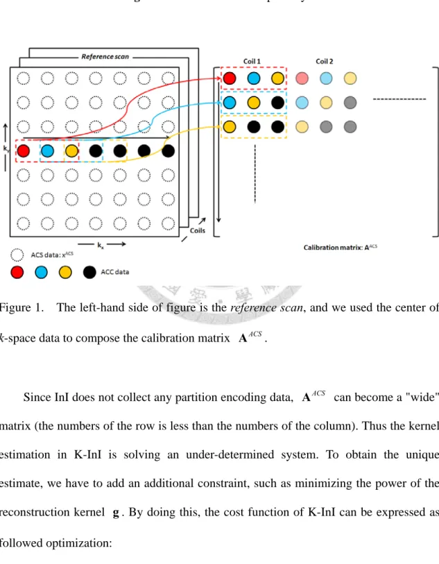
Figure 1. The left-hand side of figure is the reference scan, and we used the center of k-space data to compose the calibration matrix A^ACS.

Since InI does not collect any partition encoding data, A^ACS can become a "wide"

matrix (the numbers of the row is less than the numbers of the column). Thus the kernel estimation in K-InI is solving an under-determined system. To obtain the unique estimate, we have to add an additional constraint, such as minimizing the power of the reconstruction kernel g . By doing this, the cost function of K-InI can be expressed as followed optimization:

(18)

2 2

arg min ^ACS − ^ACS +λ_InI

g

A g x g . [3]

λInI denotes a regularization parameter. Our previous studies (Lin et al., 2006; Lin et al., 2010; Lin et al., 2008a; Lin et al., 2008b) suggested that λ_InI can be reasonably estimated from a pre-specified SNR of the measurement:

( )

²

ACSH ACS

InI

Tr

Tr SNR

λ = A A

C , [4]

where the superscript H denotes the complex conjugate and transpose, C denotes the noise covariance matrix across different channels in the RF coil array.

Eq. [1] can be solved analytically:

(

^ACS

) (

^H

(

^ACS

)

^H ^ACS ^λ^InI

)

⁻¹ ^ACS

=

g A A A + C x [5]

The estimation of reconstruction kernel is similar to the minimum-norm estimates (MNE) of the InI data (Lin et al., 2006; Lin et al., 2008a; Lin et al., 2008b). The diagram in Figure 2 shows how we reconstruct x^ACC using the accelerated functional scan A^ACC after estimating the reconstruction kernel g . A reconstructed image I^recon can be reconstructed by using the sum-of-squares (SoS) combination across all channels of the coil array:

(19)

{ }

1

1 channels recon

j j

−

=



I F x [6]

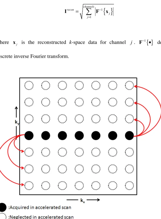
where x is the reconstructed k-space data for channel j . _j ^F⁻¹

{ }

^• denotes the discrete inverse Fourier transform.

Figure 2. K-InI reconstruction uses the phase encoding data at the k-space center AACC to interpolate the skipped k-space data.

(20)

2.4.2 Self-consistent K-InI

Iterative self-consistent parallel imaging reconstruction (SPIRiT) (Lustig and Pauly, 2010) is a k-space parallel MRI reconstruction algorithm. The self-consistent property includes two parts: the calibration consistency and the data consistency. The calibration consistency means that the linear relationship between the ACS and the ACC data, as well as non-acquired k-space and acquired k-space, should be consistent as described by Eqs. [1] and [2]. In other words, the reconstruction kernel estimated from Eq. [1] should be applied to synthesize the skipped k-space in Eq. [2]. This calibration consistency property can be further generalized by enforcing the consistency at every k-space data point: each k-space data point can be linearly synthesized from its neighboring k-space data points in all channels of an RF coil array. In K-InI, Eq. [1] defines different sets of linear correlation between the acquired k-space data points and the skipped k-space data points. In contrast, the calibration consistency in SPIRiT only defines one set of linear correlation between the acquired k-space data points and the skipped k-space data points.

SPIRiT uses the same reconstruction coefficient g to interpolate the skipped k-space data points. Let G be a convolution matrix constructed by reconstruction kernel g , we can rewrite Eq. [1]:

ACS = ACS

x Gx . [7]

Practically, the matrix G acts as a series of convolution over x to synthesize every k-space data point from its neighbors. Without the loss of generality, the calibration consistency can be expressed as:

(21)

=

x Gx. [8]

The second consistent property is the data consistency: the ideal reconstructed data should be consistent with the empirically acquired data. This constraint can be formulated as:

=

y Dx , [9]

where x denotes the ideal reconstructed k-space data, y denotes the empirically acquired k-space data, and the matrix D denotes the k-space sampling pattern (selecting the actually acquired k-space data points over the k-space grid). Eq. [8] and Eq. [9] respectively describe the calibration consistency constraint and data consistency constraint using a set of linear equations. Considering the realistic contaminating noise, these two sets of linear equations be formulated together as an optimization problem (Lustig and Pauly, 2010):

2

minimize

subject to ε

−

− ≤

Gx x

Dx y , [10]

where the parameter ε demotes the error used to control the balance between two consistency constraints. Eq. [10] can be reformulated as an unconstrained Largrangain form:

2 2

arg min − +λ_ε −

x

Dx y Gx x , [11]

(22)

where λε denotes a regularization term. A previous study (Lustig and Pauly, 2010) suggested that in the Cartesian sampling, we can incorporate the acquired k-space data in the reconstruction to completely enforce the data consistency constraint (ε =0). In this case, only the calibration consistency term Gx− x ²needs to be minimized. Let x

be a vector representing only the skipped k-space data points and y be a vector of the acquired k-space data points. Furthermore, let D denote the k-space sampling pattern _c for the skipped data on the k-space grid. Let D and ^T D respectively denote to the ^T_c linear operation of putting the acquired and reconstructed k-space data points in the right location in the k-space grid. x can be represented as:

T T

= + c

x D y D x . [12]

Substituting x into Eq. [11][11], the optimization becomes:

2

arg min ( − ) ^T_c +( − ) ^T

x

G I D x G I D y



 , [13]

Eq. [13] can be represented as a least-squares problem:

arg min − 2 x

Ax b



 , [14]

where A=(G I D and − ) ^T_c b= −(G I D y . With the reconstruction kernel g and − ) ^T

(23)

thus G, we can solve Eq. [14] iteratively by the conjugated gradient (CG) method (Shewchuk, 1994).

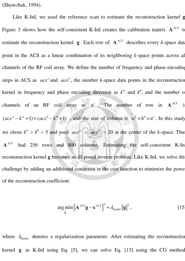
Like K-InI, we used the reference scan to estimate the reconstruction kernel g.

Figure 3 shows how the self-consistent K-InI creates the calibration matrix AÂCS to estimate the reconstruction kernel g . Each row of AÂCS describes every k-space data point in the ACS as a linear combination of its neighboring k-space points across all channels of the RF coil array. We define the number of frequency and phase encoding steps in ACS as acs and ^w acs , the number k-space data points in the reconstruction ^h kernel in frequency and phase encoding direction as k^w and k^h, and the number of channels of an RF coil array as n . The number of row in ^c AÂCS is (acs^w− k^w+1) × (acs^h− k^h+1) , and the size of column is w^k× × . In this study, h^k n^c we chose k^w = k^h = 5 and used acs = ^w acs = 20 at the center of the k-space. Thus ^h

AACS had 256 rows and 800 columns. Estimating the self-consistent K-InI reconstruction kernel g becomes an ill-posed inverse problem. Like K-InI, we solve this challenge by adding an additional constraint in the cost function to minimize the power of the reconstruction coefficient:

2 2

kernel

arg min ^ACS − ^ACS +λ

g

A g x g , [15]

where λ_kernel denotes a regularization parameter. After estimating the reconstruction kernel g as K-InI using Eq. [5], we can solve Eq. [13] using the CG method.

Reconstructions minimizing Eq. [13] is called the self-consistent K-InI.

(24)

2.4.3 ₁-self-consistent K-InI reconstruction theory

The SPIRiT optimization can alternatively use the ₁-norm minimization. This yields the ^₁−SPIRiT method:

2 1

arg min ( − ) ^T_cx+( − ) ^T +λΨ Ψ ⁻ ( ^T + ^T_c )1 x

G I D G I D y F D y D x



  , [16]

where λΨ denotes the regularization parameter, and Ψ denotes a sparsifying transformation. Practically, the sparsifying transformation in this study is the Daubechies 4 wavelet transform (Lustig et al., 2009). We used the projection on convex set (POCS) method to minimize Eq. [16] iteratively (Lustig et al., 2009).

Reconstructions minimizing Eq. [16] is called ₁-self-consistent K-InI.

Figure 3. The reconstruction kernel describes the linear relationship between each data point in k-space and its neighbors. We select the center of the reference scan as the ACS, and use the ACS to construct the calibration matrix A^ACS.

(25)

2.5 Performance measures

2.5.1 Reconstruction error analysis

We used the root mean squared error (RMSE) between the reconstructed image

recon

I and the reference data I to quantify the quality of the reconstructed image: ^ref

( )

²

1

RMSE 1

pixels

ref recon

n n₌

=



^I −^I ^{. [17]}

The reconstructed image was the sum-of-squares image from all channels of the RF coil array. Practically, we used the reference scan to simulate the InI acquisition by discarding all partition encoded data except the central partition, which was used to reconstruct images using K-InI, self-consistent K-InI and ₁- self-consistent K-InI methods.

2.5.2 Spatial resolution analysis

Similar to the reconstruction error analysis, we used numerical simulation to evaluate the localization accuracy and the spatial resolution of K-InI, the self-consistent K-InI and ₁ -self-consistent K-InI methods. We first manually selected two regions-of-interest (ROIs): one is at the visual cortex (V) and the other one is at the sensorimotor (SM) cortex of the left hemisphere. All image voxels within ROIs were set to 1 and the other voxels were set to 0. Then the image was multiplied with the image of each channel of the coil array in the reference scan voxel-by-voxel and integrated along the InI encoding direction to simulate the ideal InI measurement s. To approximate

(26)

realistic measurements, we created 100 realizations of the noise with the spatial coloring according to the noise covariance matrix C:

T c c c

12 12 T

c c

12 w

C = U L V C = L U

n = C n

, [18]

where n denoted a complex noise vector with independent zero-mean Gaussian noise _w with unit variance, and the noise covariance matrix C was estimated from the residual of the GLM analysis (see Data analysis section). With the pre-defined SNR = 1, 2, 5, 10, 20, 50, and 100, the noise n was scaled properly and added to the ideal measurement

s as follows:

( ) ( )

max 2

1

noisy

SNR Tr c

= + s

s s n

L . [19]

We used the averaged point spread function (APSF) and the SHIFT (Lin et al., 2006;

Lin et al., 2010; Lin et al., 2008a; Lin et al., 2008b) metrics to quantify the reconstruction performance. The APSF is defined as:

( ) ( )

recon

APSF

r r r

r r

r

=



r



d I

I [20]

(27)

where d_r denotes the distance between the reconstructed source at location r and

( )

recon

r r

I denotes the reconstructed image with voxel value exceeding 50% of the maximum. The localization accuracy was quantified by calculating the shift between the center of the chosen ROI and the reconstruction:

( ) ( ) ( )

recon

SHIFT

r r

c r r

r

ρ

= −

 

 

 



I I



[21]

where ^{c r}^

( )

denotes the 3D coordinate of the reconstruction and ρ denotes the center of the simulated ROI.

All calculations were implemented in MATLAB (Mathworks, Natick, MA, USA) using a Linux workstation with 1.60 GHz CPU and 64 Gbytes RAM. The image reconstruction was modified from the software package (http://www.eecs.berkeley.edu/~mlustig/software) (Lustig and Pauly, 2010). We chose the ACS size as 20 x 20 from the center of the k-space of the reference scan, the reconstruction kernel size was 5 x 5, and λΨ was 0.0015 for the ₁-norm penalty.

Since iterative reconstruction is required for self-consistent K-InI and ₁-self-consistent K-InI, the image was constructed with either a zero vector or K-InI reconstruction as the initial value.

(28)

Chapter 3 Result

3.1 Image reconstruction analysis

Figure 4 shows the RMSEs between the sum-of-squares image in the reference scan and the reconstructed images using K-InI, self-consistent K-InI, and

1-self-consistent K-InI methods with a zero-value vector as the initial value. The RMSE of K-InI was 0.0182. The RMSE of the self-consistent K-InI decreased from 0.0429 to 0.0310 after 20 iterations and to 0.0253 after 160 iterations. The RMSE of the

1-self-consistent K-InI decreased from 0.0428 to 0.0321 after 40 iterations and then diverged. This divergence is likely due to the iterative calculation of Eq. [13] using only minimally acquired InI data and the estimated reconstruction kernel g . Figure 5 shows the RMSEs of the reconstructions using self-consistent K-InI, and ₁-self-consistent K-InI methods using K-InI reconstruction result as the initial value in the iterative calculation. The RMSE of self-consistent K-InI decreased from 0.0184 to 0.0179 after 20 iterations.

(29)

Figure 4. The RMSE of the reconstructed images using K-InI, self-consistent K-InI and ₁-self-consistent K-InI methods when the reconstruction was initialized by a zero vector.

(30)

Figure 5. The RMSE of the reconstructed images using K-InI, self-consistent K-InI and ₁-self-consistent K-InI methods when the reconstruction was initialized by the K-InI reconstruction.

(31)

The top row of Figure 6 shows the trans-axial sum-of-squares image in the reference scan (Ref) and after K-InI reconstruction. Panels A - D show the reconstructed trans-axial images using self-consistent K-InI and ₁-self-consistent K-InI methods using either a zero-vector or K-InI reconstruction as the initial value after 20, 40, 80, and 160 iterations. The corresponding RMSE’s of the reconstructions were also shown in the figure. K-InI reconstructed image was found similar to the sum-of-squares reference image. But images reconstructed by self-consistent K-InI and

1-self-consistent K-InI were blurred. Using K-InI reconstruction as the initial value can improve both self-consistent K-InI and ₁-self-consistent K-InI reconstructions by showing a smaller RMSE. However, ₁-self-consistent K-InI shows strong streak artifacts along the InI accelerated direction after 40 iterations. In summary, considering the convergence and the computational loading, both self-consistent K-InI and

1-self-consistent used 20 iterations with a zero-vector as the initial value in this study.

(32)

Figure 6. The sum-of-squares reference image (SoS) and K-InI reconstruction. Panels A and B show the self-consistent K-InI and the ₁-self-consistent K-InI reconstruction after 20, 40, 80, and 160 iterations using a zero-vector as the initial value. Panels C and

(33)

D show the self-consistent K-InI and the ₁-self-consistent K-InI reconstruction after 20, 40, 80, and 160 iterations using K-InI reconstruction as the initial value.

3.2 Spatial resolution analysis

Figure 7 and Figure 8 show the reconstructed visual cortex images with simulated SNR = 1, 10, and 100 using K-InI, self-consistent K-InI, and ₁-self-consistent K-InI methods. All of them revealed similar visual cortex distribution with blurring along InI encoding direction. Three methods were found insensitive to the noise at the simulated SNR. The reconstructions by self-consistent K-InI, and ₁-self-consistent K-InI are more spatially homogeneous.

(34)

Figure 7. The reconstructed visual cortex images of K-InI, self-consistent K-InI, and

1-self-consistent K-InI at different SNRs. Reconstructions were linearly scaled between 0 and 1 to illustrate the spatial distribution. The simulated visual cortex ROI is shown as the green area.

(35)

Figure 8. The reconstructed visual cortex (V) on the inflated left hemisphere. The dark and light gray on the inflated hemisphere represent sulci and gyri of the brain respectively. The transparent green overlay at the top image and the green circles overlaid on the reconstructed images show the simulated visual cortex. Columns A, B, and C correspond to K-InI, self-consistent K-InI, and ₁ -self-consistent K-InI reconstructions.

(36)

We calculated the APSF and SHIFT metrics to quantify the localization accuracy of reconstructions. Figure 9A shows the APSF metrics for K-InI, the self-consistent K-InI, and ₁-self-consistent K-InI reconstructions. We found that the self-consistent K-InI reconstructions have the APSF smaller than 14 mm across SNRs. The APSF of

1-self-consistent K-InI was smaller than 18 mm, and the APSF of K-InI was smaller than 17 mm. The spatial dispersion for the self-consistent K-InI and K-InI was comparable, while ₁-self-consistent K-InI has the highest spatial resolution quantified by APSF. Figure 9B shows the SHIFT metric. We found that the self-consistent K-InI and ₁-self-consistent K-InI reconstructions both had smaller SHIFT metrics than K-InI. When the SNR was higher than 5, the localization precision quantified by the SHIFT metric for self-consistent K-InI and ₁-self-consistent K-InI were found to be approximately 2 mm, while K-InI has larger localization error (SHIFT > 5 mm). Overall, self-consistent K-InI and ₁-self-consistent K-InI provide more accurate localization than K-InI.

(37)

Figure 9. The APSF and SHIFT metrics for K-InI, self-consistent K-InI, and

1-self-consistent K- InI reconstructions at visual cortex (V) at different SNRs.

(38)

Figure 10 and Figure 11 show the reconstructed sensorimotor cortex images with simulated SNR = 1, 10, and 100 using K-InI, self-consistent K-InI, and

1-self-consistent K-InI methods on brain volume and the inflated brain. Like visual cortex reconstruction, three reconstructions blurred along InI encoding direction. In Figure 10, we found that K-InI significantly shift laterally while self-consistent K-InI and ₁-self-consistent K-InI shows mostly blurring.

(39)

Figure 10. The reconstructed sensorimotor (SM) cortex images of K-InI, self-consistent K-InI, and ₁-self-consistent K-InI at different SNRs. Reconstructions were linearly scaled between 0 and 1 to illustrate the spatial distribution. The simulated sensorimotor cortex ROI is shown as the green area.

(40)

Figure 11. The reconstructed sensorimotor cortex (SM) on the inflated left hemisphere.

The dark and light gray on the inflated hemisphere represent sulci and gyri of the brain respectively. The transparent green overlay at the top image and the green circles overlaid on the reconstructed images show the simulated visual cortex. Columns A, B, and C correspond to K-InI, self-consistent K-InI, and ₁-self-consistent K-InI

(41)

reconstructions.

Figure 12 shows the APSF and SHIFT metrics for the simulated source at the sensorimotor cortex (SM). The APSF of K-InI (40 mm) is about three times larger than that of self-consistent K-InI (12 mm) and ₁-self-consistent K-InI reconstruction (15 mm). In average, the spatial resolution quantified by APSF suggested that self-consistent K-InI and ₁-self-consistent K-InI reconstructions have higher spatial resolution. For localization accuracy, the SHIFT metric for K-InI, self-consistent K-InI, and ₁-self-consistent K-InI were 25 mm, 5 mm, and 7 mm respectively. The self-consistent InI and the ₁-self-consistent InI reconstructions have much higher localization accuracy than K-InI.

(42)

Figure 12. The APSF and SHIFT metrics for K-InI, self-consistent K-InI, and

1-self-consistent K-InI reconstructions at the sensorimotor cortex (SM) across different

(43)

SNRs.

3.3 In vivo experiments

Figure 13 shows the dSPM of the visual cortex BOLD responses using the group-average data (n = 6) reconstructed by K-InI, self-consistent K-InI, and

1-self-consistent K-InI methods. This figure shows that the visual activation started from 2.2 s after the onset of the visual stimulation (using t = 8 as the threshold ; uncorrected p-value < 10^-4). These three reconstruction methods revealed similar spatial distribution of the activated visual cortex but ₁-self-consistent K-InI revealed more significant BOLD activity in the visual cortex between 4.0 second to 4.9 second after the stimulus onset.

(44)

Figure 13. Group averaged event-related activity on the medial side of inflated left hemisphere. The critical threshold was t > 8 and uncorrected p-value < 10^-4. All the cropped areas from K-InI, the self-consistent K-InI and the ₁-self-consistent K-InI are indicated by the white dash rectangular area at the top image.

(45)

The time courses of the hemodynamic responses are shown in Figure 14. The shape of the estimated hemodynamic response revealed by self-consistent K-InI and K-InI are similar. Note that the estimated hemodynamic response revealed by

1-self-consistent K-InI has higher peak t-value (31) than self-consistent K-InI and K-InI reconstructions (21). This amounts to 50% increase in the sensitivity to BOLD signal.

Figure 14. The averaged hemodynamic responses of K-InI (blue), the self-consistent InI (green), and the ₁-self-consistent InI (red) at visual cortex. The ROI of visual cortex is shown in transparent green at medial side of the inflated left hemisphere.

(46)

Chapter 4 Discussion

In this study, we propose to incorporate the self-consistency property to reconstruct InI acquisitions to obtain self-consistent and ₁-self-consistent K-InI reconstructions.

Our simulations show that the reconstructed images using self-consistent and

1-self-consistent K-InI methods showing a larger RMSE than K-InI (Figure 4). We specifically observed that the RMSE of ₁-self-consistent K-InI diverged after 40 iterative reconstructions, implying that the ₁ -norm constraint may not stable.

Particularly, we found strong streak artifacts (Figure 6). We found that using K-InI as the initial value for self-consistent and the ₁-self-consistent K-InI reconstruction can get a smaller RMSE than those using a zero vector as the initial value.

To explain the reason of reconstructing images with diverged RMSE with strong streak artifacts over many iterations, it is useful to specifically contrast between self-consistent K-InI and K-InI. Self-consistent K-InI as well as ₁-self-consistent K-InI are different from K-InI in both reconstruction kernel g estimation and skipped data interpolation. K-InI has to create different reconstruction kernels, each of which accounts for a specific sampling pattern relating ACC data and the skipped k-space data point to be interpolated. This is usually an ill-posed inverse problem. After estimating the K-InI reconstruction kernels using ACS data, interpolating skipped data points from ACC is straightforward and well-defined. Differently, there is only one reconstruction kernel g for both self-consistent K-InI and the ₁ -self-consistent K-InI. Thus estimating g from ACS data is more constrained than K-InI. Given the estimated g , we then have to use calibration consistency constraint to reconstruct the image (Eq. [13]

and Eq. [16]). The process can be very ill-posed, because InI only collects the central

(47)

partition of the 3D k-space. The ill-poseness of this calibration consistency is one reason to account for the divergence of the reconstruction as iteration continues.

The estimation of the reconstruction kernel g in this study (Eq.[15]) is an ill-posed inverse problem because of the number of channels in the coil array, the chosen size of the reconstruction kernel, and the size of the ACS data. Thus Tikhonov regularization is needed for reconstruction kernel estimation (Bydder and Jung, 2009;

Qu et al., 2006). Here we used a prior constraint to minimize the power of the reconstruction kernel to obtain the unique estimate of g (Eq. [15]). However, it is possible to transform this kernel estimation into a well-posed inverse problem. This can be done by 1) increase the size of the ACS data, 2) decrease the size of the reconstruction kernel, and 3) using coil compression technique to reduce the number of the coils virtually (Buehrer et al., 2007; Doneva and Bornert, 2008; King et al., 2010;

Zhang et al., 2012). However, these options respectively have the potential issue of 1) using noisy data at the periphery of the k-space and thus reduce the stability of the reconstruction kernel, 2) reducing the degree of freedom of employing more neighboring k-space data to better interpolate the skipped k-space data points, and 3) losing part of the information from all channels of the coil array for data interpolation.

Thus the optimal configuration of the reconstruction kernel needs to be further studied.

Our ₁-self-consistent K-InI results corroborate a recent study using the ₁-norm minimization to reconstruct highly accelerated fMRI data (Hugger et al., 2011). While our method is based on k-space data interpolation, the work by Hugger et al is an image-domain reconstruction method. However, both methods show that using the

1-norm minimization can improve the spatial resolution. Moreover, Hugger et al found that replacing the wavelet transform by an identity matrix in Eq. [16] generated similar

(48)

results. We expect that we may get similar results and slightly improve the computational time by removing the wavelet transform, since the wavelet transform is a very fast process.

Since self-consistent K-InI and ₁-self-consistent K-InI methods are iterative reconstruction methods, the computational load is higher than the analytical K-InI reconstruction method. The computation time of the self-consistent K-InI and the

1-self-consistent K-InI for reconstructing a 2D slice using 32-channel coil array data is about 1 second for one iteration. It took about 10 to 20 minutes to reconstruct a 3D volumetric data with 20 iterations. In contrary, K-InI took 30 to 40 s to reconstruct a 3D data set. This computational efficiency is expected to be improved by, for example, the coil compression technique (Buehrer et al., 2007; Doneva and Bornert, 2008; King et al., 2010; Zhang et al., 2012), which can reduce the number of channels in an RF coil array into fewer virtual channels. The self-consistent GRAPPA (SC-GRAPPA) (Ding et al., 2012) has been proposed to combine traditional GRAPPA reconstruction and the self-consistency with a closed form solution. This may be used in self-consistent K-InI to reduce the computational time. Alternatively, using parallel computational architecture, such as GPGPU (Murphy et al., 2012), may further reduce the reconstruction time.

In conclusion, we demonstrate two iterative reconstruction methods using self-consistent property to reconstruct highly accelerated InI data in k-space. The results show improved spatial resolution and higher sensitivity in detecting brain areas in BOLD fMRI experiment. These reconstruction methods may help researchers to better understand the temporal details of hemodynamic response functions.

(49)

REFERENCE

Belliveau, J., Kennedy, D., McKinstry, R., Buchbinder, B., Weisskoff, R., Cohen, M., Vevea, J., Brady, T., Rosen, B., 1991. Functional mapping of the human visual cortex by magnetic resonance imaging. Science 254, 716-719.

Blaimer, M., Breuer, F., Mueller, M., Heidemann, R.M., Griswold, M.A., Jakob, P.M., 2004. SMASH, SENSE, PILS, GRAPPA: how to choose the optimal method. Top Magn Reson Imaging 15, 223-236.

Brainard, D.H., 1997. The Psychophysics Toolbox. Spat Vis 10, 433-436.

Buehrer, M., Pruessmann, K.P., Boesiger, P., Kozerke, S., 2007. Array compression for MRI with large coil arrays. Magnetic resonance in medicine : official journal of the Society of Magnetic Resonance in Medicine / Society of Magnetic Resonance in Medicine 57, 1131-1139.

Bydder, M., Jung, Y., 2009. A nonlinear regularization strategy for GRAPPA calibration.

Magnetic resonance imaging 27, 137-141.

Dale, A.M., Fischl, B., Sereno, M.I., 1999. Cortical surface-based analysis. I.

Segmentation and surface reconstruction. Neuroimage 9, 179-194.

de Zwart, J.A., van Gelderen, P., Kellman, P., Duyn, J.H., 2002. Reduction of gradient acoustic noise in MRI using SENSE-EPI. Neuroimage 16, 1151-1155.

Ding, Y., Xue, H., Chang, T.-c., Guetter, C., Simonetti, O., 2012. Self-consistent GRAPPA Reconstruction with Close-form Solution. Proceedings 20th Scientific Meeting, International Society for Magnetic Resonance in Medicine

Australia.

Doneva, M., Bornert, P., 2008. Automatic coil selection for channel reduction in SENSE-based parallel imaging. MAGMA 21, 187-196.

Farzaneh, F., Riederer, S.J., Pelc, N.J., 1990. Analysis of T2 limitations and off-resonance effects on spatial resolution and artifacts in echo-planar imaging. Magn Reson Med 14, 123-139.

Fischl, B., Liu, A., Dale, A.M., 2001. Automated manifold surgery: constructing geometrically accurate and topologically correct models of the human cerebral cortex.

IEEE Trans Med Imaging 20, 70-80.

Fischl, B., Sereno, M.I., Dale, A.M., 1999. Cortical surface-based analysis. II: Inflation, flattening, and a surface-based coordinate system. Neuroimage 9, 195-207.

Golay, X., de Zwart, J.A., Ho, Y.C., Sitoh, Y.Y., 2004. Parallel imaging techniques in functional MRI. Top Magn Reson Imaging 15, 255-265.

Griswold, M.A., Jakob, P.M., Chen, Q., Goldfarb, J.W., Manning, W.J., Edelman, R.R., Sodickson, D.K., 1999. Resolution enhancement in single-shot imaging using simultaneous acquisition of spatial harmonics (SMASH). Magn Reson Med 41, 1236-1245.

Griswold, M.A., Jakob, P.M., Heidemann, R.M., Nittka, M., Jellus, V., Wang, J., Kiefer, B., Haase, A., 2002. Generalized autocalibrating partially parallel acquisitions (GRAPPA). Magn Reson Med 47, 1202-1210.

Hennig, J., Zhong, K., Speck, O., 2007. MR-Encephalography: Fast multi-channel monitoring of brain physiology with magnetic resonance. Neuroimage 34, 212-219.

Hugger, T., Zahneisen, B., LeVan, P., Lee, K.J., Lee, H.L., Zaitsev, M., Hennig, J., 2011.

Fast undersampled functional magnetic resonance imaging using nonlinear regularized parallel image reconstruction. PLoS One 6, e28822.

Jakob, P.M., Griswold, M.A., Edelman, R.R., Sodickson, D.K., 1998. AUTO-SMASH:

(50)

a self-calibrating technique for SMASH imaging. SiMultaneous Acquisition of Spatial Harmonics. MAGMA 7, 42-54.

King, S.B., Varosi, S.M., Duensing, G.R., 2010. Optimum SNR data compression in hardware using an Eigencoil array. Magnetic resonance in medicine : official journal of the Society of Magnetic Resonance in Medicine / Society of Magnetic Resonance in Medicine 63, 1346-1356.

Kwong, K.K., Belliveau, J.W., Chesler, D.A., Goldberg, I.E., Weisskoff, R.M., Poncelet, B.P., Kennedy, D.N., Hoppel, B.E., Cohen, M.S., Turner, R., et al., 1992. Dynamic magnetic resonance imaging of human brain activity during primary sensory stimulation.

Proc Natl Acad Sci U S A 89, 5675-5679.

Lin, F.H., Wald, L.L., Ahlfors, S.P., Hamalainen, M.S., Kwong, K.K., Belliveau, J.W., 2006. Dynamic magnetic resonance inverse imaging of human brain function. Magn Reson Med 56, 787-802.

Lin, F.H., Witzel, T., Chang, W.T., Wen-Kai Tsai, K., Wang, Y.H., Kuo, W.J., Belliveau, J.W., 2010. K-space reconstruction of magnetic resonance inverse imaging (K-InI) of human visuomotor systems. Neuroimage 49, 3086-3098.

Lin, F.H., Witzel, T., Mandeville, J.B., Polimeni, J.R., Zeffiro, T.A., Greve, D.N., Wiggins, G., Wald, L.L., Belliveau, J.W., 2008a. Event-related single-shot volumetric functional magnetic resonance inverse imaging of visual processing. Neuroimage 42, 230-247.

Lin, F.H., Witzel, T., Zeffiro, T.A., Belliveau, J.W., 2008b. Linear constraint minimum variance beamformer functional magnetic resonance inverse imaging. Neuroimage 43, 297-311.

Lustig, M., Alley, M., Vasanawala, S., Donoho, D., Pauly, J., 2009. L1 SPIR-iT:

Autocalibrating Parallel Imaging Compressed Sensing. Proceedings 17th Scientific Meeting, International Society for Magnetic Resonance in Medicine, Honolulu, p. 379.

Lustig, M., Pauly, J.M., 2010. SPIRiT: Iterative self-consistent parallel imaging reconstruction from arbitrary k-space. Magn Reson Med 64, 457-471.

Mansfield, P., 1977. Multi-planar image formation using NMR spin echoes. Journal of Physics C: Solid State Physics 10, L55.

McGibney, G., Smith, M.R., Nichols, S.T., Crawley, A., 1993. Quantitative evaluation of several partial Fourier reconstruction algorithms used in MRI. Magn Reson Med 30, 51-59.

Murphy, M., Alley, M., Demmel, J., Keutzer, K., Vasanawala, S., Lustig, M., 2012. Fast l(1) -SPIRiT Compressed Sensing Parallel Imaging MRI: Scalable Parallel Implementation and Clinically Feasible Runtime. Ieee Transactions on Medical Imaging 31, 1250-1262.

Noll, D.C., Nishimura, D.G., Macovski, A., 1991. Homodyne detection in magnetic resonance imaging. IEEE Trans Med Imaging 10, 154-163.

Ogawa, S., Lee, T.M., Kay, A.R., Tank, D.W., 1990. Brain magnetic resonance imaging with contrast dependent on blood oxygenation. Proc Natl Acad Sci U S A 87, 9868-9872.

Pelli, D.G., 1997. The VideoToolbox software for visual psychophysics: transforming numbers into movies. Spat Vis 10, 437-442.

Pruessmann, K.P., Weiger, M., Scheidegger, M.B., Boesiger, P., 1999. SENSE:

sensitivity encoding for fast MRI. Magn Reson Med 42, 952-962.

Qu, P., Wang, C., Shen, G.X., 2006. Discrepancy-based adaptive regularization for GRAPPA reconstruction. J Magn Reson Imaging 24, 248-255.

Roemer, P.B., Edelstein, W.A., Hayes, C.E., Souza, S.P., Mueller, O.M., 1990. The

(51)

NMR phased array. Magn Reson Med 16, 192-225.

Shewchuk, J.R., 1994. An Introduction to the Conjugate Gradient Method Without the Agonizing Pain. Carnegie Mellon University.

Sodickson, D.K., Manning, W.J., 1997. Simultaneous acquisition of spatial harmonics (SMASH): fast imaging with radiofrequency coil arrays. Magn Reson Med 38, 591-603.

Zhang, T., Pauly, J.M., Vasanawala, S.S., Lustig, M., 2012. Coil compression for accelerated imaging with Cartesian sampling. Magnetic resonance in medicine : official journal of the Society of Magnetic Resonance in Medicine / Society of Magnetic Resonance in Medicine.