抽取謂詞以改進性質導向可達性技術

(1)

(2)

(3)

誌謝

終於到了求學生涯的一個斷點，雖然不知道之後會不會有機會再回歸校園生活，但目前來說也是該到外面去闖一闖了。

感謝我的指導教授黃鐘揚老師，有幸跟了你三年，能體會到如此開明的風氣，自由選擇研究的方向，也不會特地訂立強硬的期限或繁雜的規則，讓我們隨心所欲之餘也給予適時的提點，才不至於迷失方向，中間儘管遭遇些許失敗的挫折，最後也還是完成了這份論文。

感謝實驗室的各位，不管是已經畢業的學長姐或是還在實驗室的同學和助理，有問題的時候有人可以一起解決是很幸運的事情。

感謝我的朋友們，從高中到大學再到研究所，雖然沒有太多特別激情的回憶，只是重複著平淡的事情，但身邊有你們的陪伴的確讓人安心不少。

最後要感謝我的父母，不辭勞苦的把我養大，供我念書，離開家裡來念大學已經六年了，偶爾仍會感到非常思念，在我最低落的時候我總是相信還有你們會支持我，你們是我繼續堅持往下最大的動力。

畢業雖然是個結束，卻也是個新的開始，希望未來的我能活得精采快樂，不負現在的努力。

(4)

中文摘要

自從在 2011 年被提出後，性質導向可達性技術至今仍是最好的模型檢查演算法。但是仍有許多的案例是性質導向可達性技術難以解決的，因此，為了改進這個演算法，有許多的研究先後被發表。在這篇論文中，我們藉由獨立的檢查謂詞以輔助性質導向可達性演算法。此外，作為證明的例子，我們也提供了兩種能夠輕易從演算過程中得出的樣式。原本的性質導向可達性演算法與新方法皆被實作於 Ia2b 這個自製的模型檢查環境上。透過利用硬體模型檢查比賽的資料所做的實驗得知，我們所提出的方法能夠解出比原本的性質導向可達性技術更多的案例。

關鍵字：正規驗證、模型檢查、可滿足性問題、性質導向可達性技術、謂詞修正

(5)

Abstract

Since proposed in 2011, PDR (IC3) has been the best model checking algorithm until now. However, there are still many cases that PDR struggles to solve. Hence, many works are presented to enhance the algorithm. In this thesis, we propose a general method to aid PDR by solving predicate separately. Furthermore, we provide two kinds of useful pattern easily recognized from the solving process as example. The original PDR algorithm and the new feature are implemented on a custom model checking environment called Ia2b. The experiment on HWMCC benchmarks shows that our method can solve more cases than the classic PDR.

Keywords: Formal Verification, Model Checking, Satisfiability Problem, Property Directed Reachability, Predicate Refinement

(6)

List of Figures

2.1 The depiction of trace of frame. . . 9

2.2 The depiction of recBlockCubes. . . 14

3.1 36 blocked cubes out of the 889 ones in the inductive invariant of 6s288r. 19 3.2 The depiction of the similar clause problem. . . 20

3.3 The depiction of the reason for the similar clause problem. . . 21

3.4 An example for clause-based predicate. . . 24

3.5 The possible distribution of reachable and bad states for similar obligation problem. . . 25

3.6 An example for obligation-based predicate. . . 26

3.7 The proof obligations leading to the similar clauses. . . 28

3.8 The cone of 12141 !12142 12180. . . 29

3.9 The cone of the literal along with 12141 !12142 12180 in Figure 3.1. . . . 29

3.10 Blocking procedure for the similar clauses (1). . . 30

4.1 The memory arrangement for cube of PDR. . . 34

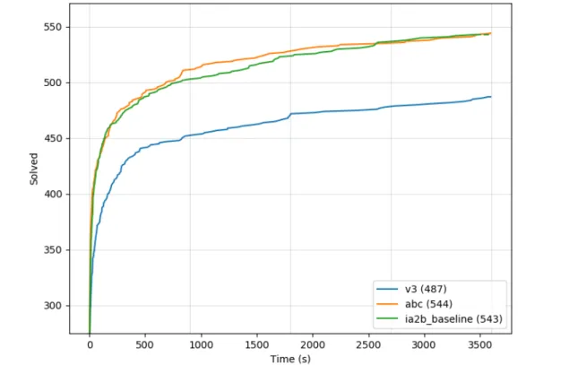
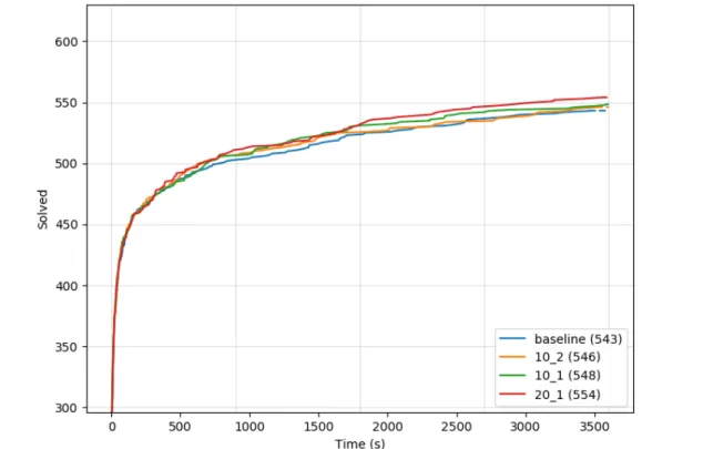
5.1 The cumulative plot of PDR among different model checkers. . . 47

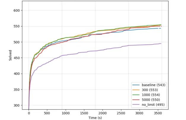
5.2 The cumulative plot of different limit of SAT query for CLS, INF, B = 20, M = 1 on pdr_vb. . . 49

(9)

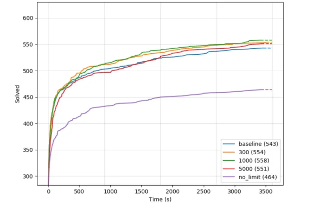
5.3 The cumulative plot of different limit of SAT query for CLS, ALL, B = 10, M = 2 on pdr_vb. . . 50 5.4 The schematic diagram of the sweet spot prediction. . . 51 5.5 The depiction of sample points. . . 51 5.6 The cumulative plot of different ratio of Backtrack number and Match

number for CLS, INF, L = 1000 on pdr_vb. . . 53 5.7 The cumulative plot of different ratio of Backtrack number and Match

number for CLS, ALL, L = 1000 on pdr_vb. . . 54 5.8 The cumulative plot of two best ratios and the mixed version for CLS, L

= 1000 on pdr_vb. . . 55 5.9 The cumulative plot of two best ratios and the mixed version for CLS, L

= 300 on pdr_vb. . . 56 5.10 The cumulative plot of different limit of SAT query for OBL, T = 66 on

pdr_vb. . . 58 5.11 The cumulative plot of different Obligation threshold for OBL, L = 300

on pdr_vb. . . 59 5.12 The cumulative plot of the best parameters for CLS, OBL and the

combination of both on full. . . 60 5.13 The comparison between clause-based and obligation-based predicate. . . 63 5.14 The comparison between basic PDR and clause-based predicate (1). . . . 64 5.15 The comparison between basic PDR and clause-based predicate (2). . . . 65 5.16 The comparison between basic PDR and obligation-based predicate. . . . 65

(10)

List of Tables

5.1 Comparison of PDR among different model checkers. . . 47 5.2 Comparison among different limit of SAT query for CLS, INF, B = 20, M

= 1 on pdr_vb. . . 49 5.3 Comparison among different limit of SAT query for CLS, ALL, B = 10,

M = 2 on pdr_vb. . . 50 5.4 Comparison among different ratio of Backtrack number and Match

number for CLS, INF, L = 1000 on pdr_vb. . . 53 5.5 Comparison among different ratio of Backtrack number and Match

number for CLS, ALL, L = 1000 on pdr_vb. . . 54 5.6 Comparison among two best ratios and the mixed version for CLS, L =

1000 on pdr_vb. . . 55 5.7 Comparison among two best ratios and the mixed version for CLS, L =

300 on pdr_vb. . . 56 5.8 Comparison among different limit of SAT query for OBL, T = 66 on pdr_vb. 58 5.9 Comparison among different Obligation threshold for OBL, L = 300 on

pdr_vb. . . 59 5.10 Comparison among the best parameters for CLS, OBL and the

combination of both on full. . . 60

(11)

Chapter 1 Introduction

Model checking is the problem to check if a specification is violated under a transition system. This kind of problem is common in the area of formal verification. For hardware verification, as the design becomes more complicated, the gate count in a circuit grows dramatically, which makes the complexity of this problem becomes higher and higher.

Hence, many innovative algorithms are proposed continually to tackle with the problem.

At early time, Binary Decision Diagram (BDD) [1] is used to compute the exact image by building the transition relation. The process continues until either a fixed point is reached or the current reachability intersects with the violation. However, BDD has poor scalability for large design since it often suffers from memory explosion.

As SAT algorithm gets tremendous efficiency improvement [2, 3, 4, 5, 6, 7], many researchers notice the practicality for SAT-based model checking method. Bounded Model Checking (BMC) [8] unfolds the circuit to check whether some states are reachable in this length. BMC itself can only answer whether the system is safe until a given length instead of proving the property completely. Afterwards, many algorithms based on BMC are proposed to enable the proof.

[9, 10] uses BMC as base case to support K-Induction (IND) for the proof. The SAT query of K-Induction also involves unrolling. Furthermore, the simple-path constraints should be added to make the algorithm complete.

(12)

In [11], McMillan shows a procedure to construct Craig’s interpolation [12] from a resolution refutation generated by modern SAT solver and use this technique to compute the over-approximated image. BMC is used for finding counter example, either real or spurious one. If BMC returns UNSAT, interpolant is computed and then sent to fixed-point checking. If the result is true, an inductive invariant set is found; otherwise, the interpolant is used for the next BMC solving. This method is called Interpolation-based Model Checking (IMC). On the other hand, Interpolation-Sequence Based Model Checking [13] works in similar way but different manner. There are also efforts to explore the property about interpolant [14, 15].

After several years, Bradley proposes a novel non-unrolling method [16] based on his previous work [17]. His implementation called IC3 won the third place in Hardware Model Checking Competition (HWMCC) 2010. Only two well-tuned integrated verification tools can beat it. Later, Eén presents a more efficient version of IC3 called Property Directed Reachability (PDR) [18]. From then on, PDR becomes the most important model checking algorithm and is commonly implemented in verification environment.

There are many works trying to modify PDR to improve it like [19, 20, 21, 22, 23].

Among them, [24] lets a blocked cube be a spurious proof obligation when it fails to be propagated to the next frame. This can be seen as over-approximating the property to let PDR refine the reachability more eagerly. However, this seems to be not so useful compared to its overhead. Hence, the authors need to include other techniques to demonstrate the potential of the method.

1.1 Contributions of the Thesis

In this thesis, we propose a general method to aid PDR by solving predicate separately.

The meaning of this method is to force PDR solve for what we guess useful instead of only the original property. PDR will search for what is actually unreachable more eagerly

(13)

since we over-approximate the property by predicates. The predicate serves as a guide to smooth the whole process of solving. This is because we find predicate by observing the solving process locally and point out what obstacle PDR encounters in this period.

By handling the obstacle separately in time, it is expected to improve the efficiency. We further provide two examples of how to produce such predicate by blocking clauses and proof obligations. Both of them can help PDR solve cases that are hardly proven by the original PDR among various implementations. Overall, PDR with predicate extraction performs better than the original one.

1.2 Organizations of the Thesis

The rest of the thesis is organized as follows. Some background knowledge is provided in chapter 2 to define the problem and method clearly. In chapter 3, we explain our method for PDR based on predicate solving. The implementation details including the whole environment and optimization are listed in chapter 4. We show the experimental results in chapter 5 to support our method. In the last chapter, we make a conclusion and discuss about the future work.

(14)

Chapter 2 Preliminaries

In this chapter, we give a seires of basic knowledge for PDR step by step to help readers realize the background.

2.1 Propositional Satisfiability

One-dimensional Boolean space is a set containing only two elements B = {T^RUE, FALSE}. Multi-dimensional Boolean space is defined by the n-ary Cartesian product Bⁿ = B×B...×B, where n is the number of dimension. A propositional variable is a variable whose value is defined onB. A literal is a propositional variable with positive or negative polarity. A cube is a conjunction of literals, while a clause is a disjunction of literals. A disjunctive normal form (DNF, also called sum of product, SOP) is a disjunction of cubes, while a conjunctive normal form (CNF, also called product of sum, POS) is a conjunction of clauses. The satisfiability (SAT) problem is to answer if there exists an assignment such that the given propositional formula is evaluated to TRUE. If the answer is yes, we call it satisfiable (SAT); otherwise, it is unsatisfiable (UNSAT). We say that a clause is satisfied if at least one literal in it is evaluated to TRUE. The given formula is usually in the form of CNF, which means the instance is SAT iff all the clauses are satisfied under the assignment.

(15)

2.2 Finite State Boolean Transition System

We can define the finite state Boolean transition system M by introducing three components ⟨S, Init, T r⟩. S is a finite set of propositional variables called state variable, and a state s is an assignment on them. Therefore, we know that the set of all states is equal toB^|S|, where the vertical bars means the cardinality of a set. Init(S) is a propositional formula to mark the initial state. That is, a state s belongs to the initial state iff Init(s) is TRUE. T r(S, S^′) is also a propositional formula, and it is used to indicate the transition relationship of the system. S^′ is a copy from S to represent the next state after transition. Given two states s₁, s₂, either identical or different, s₁ can transit to s₂ iff T r(s₁, s₂) is TRUE.

To correspond with the circuit representation that we encounter in real problem, we define an equivalent form as transition function. Consider that a state may transit to more than one state, we introduce another set of propositional variables I called input variable. Formally, the domain of the transition function isB^|S∪I| and the codomain is B^|S^′^|. The system will go to T f (s, i) under the current state s and input combination i.

To convert the transition function to the transition relation, we just perform existential quantification on the input variables. That is, T r(S, S^′) =∃I.(S^′ = T f (S, I)).

2.3 Model Checking Problem

A property p is a propositional formula to mark the set of states meeting the expectation.

A bad state is a state s such that p(s) is FALSE, and we call the rest states as good state.

Model checking can be divided to two main categories, including safety and liveness problem. Safety problem (AG p) is to answer whether the system can go a bad state or not without any time limit. On the other hand, liveness problem (AF p) checks if the system can eventually reach a good state along any branch. The algorithms introduced in this thesis focus on the safety problem. If AG p is true, we say the problem is safe

(16)

Definition 1. A trace isa finite sequence of states that all adjacent states follow the transition relation.

Definition 2. A state is reachable at k steps from another state if there exists a trace of length k such that it is the last state and the first one is that state. A state is reachable from another state if it is reachable at any step; otherwise, it is unreachable. If not specified explicitly, it means reachable from the initial state.

The safety problem can then be described as whether all the bad states are unreachable. That is, it is to show that there exists no counterexample, where a counterexample means a trace to any bad state. In order to prove this problem, we need to introduce the following two terms.

Definition 3. A set of states characterized by a propositional formula Ind is inductive iff it contains the initial state and no state belonging to it can transit out of itself.

1. Init(S)→ Ind(S) (Base)

2. Ind(S)∧ T r(S, S^′)→ Ind(S^′) (Inductive)

Definition 4. A set of states characterized by a propositional formula Inv is invariant iff it holds the property. That is, all the states belonging to it are good.

Inv(S)→ p(S)

Lemma 1. The safety problem is true iff we can find an inductive and invariant set.

The proof is trivial to show that all the bad states are not reachable at any step by

(17)

induction. Then the rest problem is how to compute the inductive invariant set. A straightforward way is to compute the set of all the reachable states, which is actually the smallest inductive set. This scheme is called exact reachability analysis, which is adapted by BDD and some SAT-based techniques like [25]. A basic procedure for exact reachability analysis is to compute the image of the current set of states until fixpoint while starting from the initial state. The image means the set of states that can transit from any state of the current set. That is, image(R) = {s^′| ∃ s ∈ R, T r(s, s^′) = TRUE} Furthermore, we say the set reaches a fixpoint if it becomes inductive and cannot transit to any other state.

Algorithm 1: safetyByExactReach

Input: Transition system M , property p Output: safe or violated

1 R← Init

2 while not R(S)∧ T r(S, S^′)→ R(S^′)

3 R← R ∨ image(R)

4 if R∧ ¬ p = SAT

5 return violated

6 else

7 return safe

However, the computing effort is too expensive so that it is undesirable to perform on large design. Instead, we compute an approximation of the reachable states in more affordable way. In order to use the approximation for proof, we need to make sure the approximation maintains an ordering relative to the image, which means one must be a subset of the other. Under-approximation assures that the approximation is contained in the image; otherwise, over-approximation ensures the approximation being a superset of the image. The modern SAT-based algorithms like IMC or PDR are usually over-approximations. We can still complete the proof if the obtained inductive set is also invariant, but we cannot answer that the property is violated otherwise since there may exist a smaller inductive set that holds the property. Whenever we encounter a counterexample, we need to verify whether it is real or just spurious. Hence, the

(18)

counterexample refinement to form a whole picture. The refinement for IMC is just discarding the current set and restart the computation after unrolling one more timeframe. On the other hand, PDR uses blocking clause to exclude the spurious counterexample and form the image simultaneously.

2.4 Property Directed Reachability

In this section, we introduce the method of basic PDR to facilitate the explanation of our method in the next chapter. The content basically follows the implementation in [18]

with proper rearrangement and renaming.

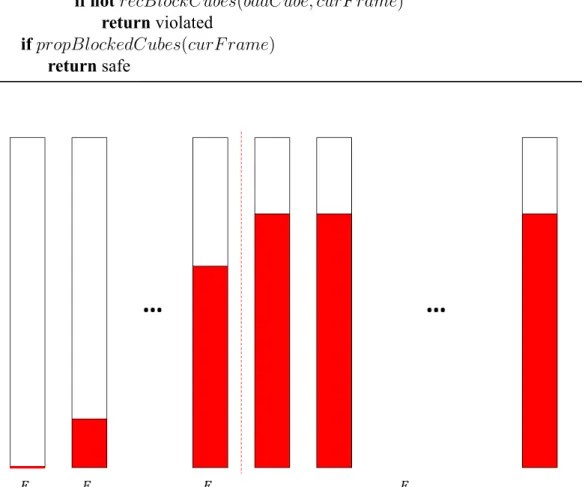
How PDR treats the reachability is to continuously refine the over-approximation whenever a spurious counterexample is found by adding clauses to refute it. Throughout the process, PDR maintains a trace of frames ⟨F0, F₁, ..., F_n⟩, where frame is a set of clauses over-approximating the states reachable at a certain step or less. The trace has the following 5 properties:

1. F₀ = Init.

2. ∀i > 0, Fi is set of clauses and is represented by the intersection of them.

3. ∀i > 0, Fi+1is a subset of F_iand all the clauses in F_icontain the initial state, which means∀i ≥ 0, Fi→ Fi+1.

4. Fi(S)∧ T r(S, S^′)→ Fi+1(S^′), Fi+1over-approximates the image of Fi. 5. F_i→ p, the frame holds the property except for the tail of the trace.

The pseudo code of the main process is shown in Algorithm 2. In addition to that the first frame F₀ is initial, we keep another special frame F_∞ that represents the current inductive set. We can always place F_∞behind the tail of the trace without violating the above 5 rules. The length of trace keeps increasing over each iteration. For each new frame except for the first one, it starts by copying the clauses from F_∞. Then we can try

(19)

to propagate the clause in the previous frame to the current one, which is performed in propBlockedCubes. The fixpoint checking is also included in this section. If there still exists a witness of violation in the last frame, we need to check if it is real or spurious.

This is done by recBlockCubes. After the tail of the trace becomes invariant, we proceed to the next frame.

Algorithm 2: safetyByPDR

Input: Transition system M , property p Output: safe or violated

1 F₀← Init

2 F_∞← T autology

3 for curF rame = 0 to∞

4 while TRUE

5 badCube← getBadCube(p, curF rame)

6 if badCube̸= N^ULL

7 if not recBlockCubes(badCube, curF rame)

8 return violated

9 if propBlockedCubes(curF rame)

10 return safe

Figure 2.1: The depiction of trace of frame. F_∞ represents all the frames beyond the current frame. When newing a frame, just add one of them into consideration.

(20)

Theorem 1. At the end of each iteration, the safety is proved by PDR if there are two adjacent frames with the same size.

P roof :

We show that the set of states of the two frames are inductive and invariant.

1. The size of the two frames are the same.

By Property 3, the two frames have the same clauses. That is, the same set of states.

|Fi| = |Fi+1| ⇒ Fi = F_i+1

By Property 4, this set is inductive.

Fi(S)∧ T r(S, S^′)→ Fi+1(S^′) = Fi(S^′)

2. At the end of iteration, all the frames holds the property. It is invariant.

F_i→ p

Hence, F_iis both inductive and invariant. By Lemma 1, the safety is proved. ■

In the following subsections, we introduce each component of PDR to explain the algorithm and its correctness more clearly.

2.4.1 The Monotonicity of Frames

Definition 5. A set of states F is inductive relative to another one G iff it contains the initial state and no state belonging to both G and F can transit out of F [17].

1. Init(S)→ F (S) (Base)

2. F (S)∧ G(S) ∧ T r(S, S^′)→ F (S^′) (Inductive)

(21)

When a cube is examined whether it is reachable at a certain frame, only the previous frame is involved. We check if there exists any state in the previous frame that can transit into the cube. If the answer is not, we can add the negation of the cube as blocking clause to block it at the frame. We will use blocking clause and blocked cube interchangeably since they are just negation of each other. A special feature for PDR about the checking is to query whether F_k₋₁(S)∧ ¬ c(S) ∧ T r(S, S^′)→ ¬ c(S^′) holds, which means ¬ c is inductive relative to Fk−1. It is the term ¬ c(S) that enables the addition of blocking clause to all the frames before the target one.

Theorem 2. If the addition of blocking clause meets the following criteria, the trace of frames holds the Property 4.

¬ c is added to F1∼ Fkif it contains the initial state and is inductive relative to Fk−1.

1. c∧ Init = UNSAT

2. F_k₋₁(S)∧ ¬ c(S) ∧ T r(S, S^′)∧ c(S^′) = UNSAT

P roof :

For simplicity, we only keep two F_∞from Figure 2.1 to preserve the inductive property of itself. For consistency of indices, we assign the two F_∞to be F_n+1and F_n+2. In addition, we assume to add the clause to the first frame even if it actually does not since this is equivalent. Then it turns out that we need to show

∀ i ∈ [0, n + 1], Fi′(S)∧ T r(S, S^′)→ Fi+1^′ (S^′),

where F_i^′ =









F_i∧ ¬ c, ∀ i ∈ [0, k]

F_i, ∀ i ∈ [k + 1, n + 2]

1. For i > k, nothing changes.

(22)

2. For i = k

Fi′(S)∧ T r(S, S^′) = Fi(S)∧ ¬ c(S) ∧ T r(S, S^′)

→ Fi(S)∧ T r(S, S^′)

→ Fi+1(S^′) = F_i+1^′ (S^′)

3. For i < k

(i) ¬ c is inductive relative to Fi

Fi′(S)∧ T r(S, S^′) = Fi(S)∧ ¬ c(S) ∧ T r(S, S^′)

→ Fk−1(S)∧ ¬ c(S) ∧ T r(S, S^′)

→ ¬ c(S^′)

(ii) Only adding¬ c to Fiholds the inductive property

F_i^′(S)∧ T r(S, S^′) = F_i(S)∧ ¬ c(S) ∧ T r(S, S^′)

→ Fi(S)∧ T r(S, S^′)

→ Fi+1(S^′)

(iii) By composition of the above two formula

F_i^′(S)∧ T r(S, S^′)→ Fi+1(S^′)∧ ¬ c(S^′) = F_i+1^′ (S^′)

Combine the three cases, we know that Property 4 holds. ■

The result is that the former frame must be a subset of the latter one (Property 3).

That is, the set of clauses monotonically decreases along the trace. Hence, in the implementation, we just record the difference of adjacent frames to prevent duplication.

In order to reuse the SAT solver, we use assumption to activate the frames and mark the

(23)

cube. For modern SAT solver, it is able to derive a final conflict clause based on the assumption. We can remove the literals that do not participate in the proof, which results in a higher frame and a larger cube.

2.4.2 Ternary Simulation

From the witness of violation in the last frame, if a cube cannot be blocked at a certain frame, we can find a state in the previous frame that cause the reachability and recursively do the blocking. We can use ternary simulation to collect more states with the same property to form a larger cube. The transition for ternary logic on AND gate includes {0 ∧ X = 0, 1 ∧ X = X, X ∧ X = X and ¬ X = X} besides the basic Boolean operation. We first define target as a set of signals with the value we want. It can also be described as a cube since all the values should hold simultaneously, but is not restricted to only state variable. In getBadCube, the target is the violation of property

¬ p. In checkReach, the target is the given cube c. Starting with a normal simulation, the value of the given state can transit to the target. Now we force one variable in the state to be X and perform the ternary simulation on the circuit. If there is no signal in the target becoming X, the changed variable is actually don’t-care so it can be set to X.

Otherwise, we need to reset the variable to its original value since it is crucial for the transition. The iteration can be performed for every state variable to find as much don’t-care as we can. We can call the obtained cube as proof obligation since the whole cube should be blocked at every frame to prove the safety. Note that this statement makes sense since the obtained cube of a proof obligation is still a proof obligation.

Lemma 2. All the states in the cube obtained by ternary simulation can transit to its target. (Only consider the variables in the target.)

(24)

2.4.3 Recursively Blocking Cubes

Starting from a witness of violation in the last frame, we need to check if it is really reachable from the initial state. From the previous subsection, we know the reachability checking only involves the previous frame. If the previous frame is strong enough to ensure the unreachability, we just add blocking clause to every corresponding frame.

However, if is too weak to refute, we still do not know whether the proof obligation is reachable or not. If we want to block the proof obligation in this frame, we first need to block the state in the previous frame that can transit to it. Hence, we extract the assignment from the SAT solver to form a new proof obligation at the previous frame. If the blocking of the new proof obligation succeeds, we can go back to the original one and try to block it again. But if it fails, just repeat the same process at more previous frames recursively. The extreme case is reaching F0, which means no refinement can be done anymore and shows the presence of a counterexample. Otherwise, at the end of the subroutine, all the frames are refined to be strong enough to block the first proof obligation in the last frame.

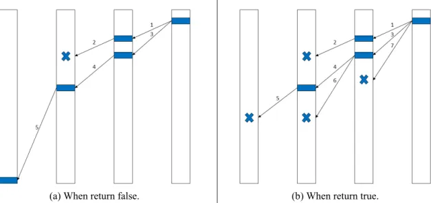
(a) When return false. (b) When return true.

Figure 2.2: The depiction of recBlockCubes. The blue rectangle means proof obligation.

The X means unreachable from the previous frame. The arrow means the reachability checking. The number associated with each arrow means the order to perform.

(25)

The process is illustrated by Algorithm 3. The most special modification is at line 16 where we push the blocked proof obligation to further frame since it should be blocked everywhere. Without this setting, the process acts as a depth first search as depicted in Figure 2.2 where the depth is between the current frame and the last one. In this situation, a stack is enough to record the trace of proof obligations. However, with this setting, there will be multiple proof obligations waiting at a frame to be blocked so that we should arrange more space to record. In addition, an integer blockF rame is introduced to indicate where the blocking takes place now. If a proof obligation should be blocked at the first frame, we know a counterexample is found and return false. We always try to block the proof obligation with the lowest frame throughout the process. When we focus on a frame, we can pick any of the proof obligation in that frame to block. First we check if it is already blocked at that frame by simply subsumption or even SAT query. We then check the reachability relative to the previous frame if the answer is not. If it is reachable from the previous frame, go to deeper frame recursively. Otherwise, add blocking clause properly after performing generalization on it. After emptying the task for a frame, go back to the shallower one. If all the proof obligations are blocked without reaching the first frame, the first one is really unreachable and true is returned. Last, we introduce the term bad depth to represent the distance of proof obligation between the last one. The bad depth of the last proof obligation is 0 since it is exactly the violation of property, while the bad depth of the rest proof obligations is one more than that of the one producing it.

2.4.4 Propagating Blocked Cubes

The process to propagate cube is illustrated in Algorithm 4. It is very simple that checking the reachability at the next frame for every blocking clause in every frame. For the detail of implementation, we only check the difference between two adjacent frames since the storage is exactly like that. To check whether the two frames are equivalent, we can just check if the number of difference between two frames is zero.

(26)

Algorithm 3: recBlockCubes

Input: Cube badCube, the frame to block f Output: TRUEor FALSE

Data: An infinite array of set of cubes badArr

1 badArr[f ].add(badCube)

2 blockF rame← f

3 while blockF rame≤ f

4 if blockF rame = 0

5 return FALSE

6 targetCube← badArr[blockF rame].pop()

7 if not isBlocked(targetCube, blockF rame)

8 preCube← checkReach(targetCube, blockF rame)

9 if preCube̸= N^ULL

10 badArr[blockF rame].add(targetCube)

11 blockF rame← blockF rame − 1

12 badArr[blockF rame].add(preCube)

13 else

14 addBlockedCube(generalize(targetCube, blockF rame))

15 if blockF rame < f

16 badArr[blockF rame + 1].add(targetCube)

17 if badArr[blockF rame].empty()

18 blockF rame← blockF rame + 1

19 return TRUE

Algorithm 4: propBlockedCubes

Input: The currently maximum frame curF rame Output: TRUEor FALSE

1 for k = 1 to curF rame

2 for all cubes c∈ Fk

3 if checkReach(c, k + 1) = NULL

4 addBlockedCube(c, k + 1)

5 if F_k = F_k+1

6 return TRUE

7 return FALSE

(27)

2.4.5 Other Subroutines

Generalization in PDR means to gain more information from a proof obligation as we can.

The information here is to block larger cube in higher frame, which means to get closer to the exact reachability. The generalization process roughly contains three phases.

1. Use the final conflict clause produced by SAT solver to remove the literals not related to the UNSAT proof, which leads to a larger cube and a higher frame. This procedure is performed in every checkReach, which means it is also activated by the rest two steps.

2. More eagerly, iteratively check the reachability by ignoring one literal at a time. If the resulting cube is still unreachable, the literal will be actually removed. Note that the cube cannot intersect with the initial state, or the criterion of correctness fails.

3. By fixing the cube, check if it is unreachable at further frame until the pushing fails.

Definition 6. A cube c1subsumes another one c2iff all the literals in c1are also in c2. {l | l ∈ c1} ⊆ {l | l ∈ c2}

Subsumption is another basic part in PDR. It is performed at two places.

1. To check a proof obligation is blocked at the frame or not. If it is subsumed by any of the blocking clause, it has already been blocked.

2. Before adding a blocking clause to the corresponding frame, all the clauses subsumed by it in that frame are removed to prevent redundancy.

(28)

Chapter 3 Predicate Extraction

In this chapter, we explain our method, property directed reachability with predicate extraction. We first describe the problem we observe and how it inspires us to come up with the solution. Then a simple general method by predicate solving is proposed with the proof of its correctness. Finally, we give two examples of predicate to demonstrate the feasibility and efficiency.

3.1 Motivation

Among various implementations of PDR, the final inductive and invariant sets are all distinct due to the don’t-cares. Although not directly related to the runtime, the number of clauses somewhat illustrates how efficiently the engine solves the problem. There may exists many possible inductive invariant sets, so the problem is how to find a proper one from them with elegant representation of clauses. Hence we collect the inductive invariant set with the form of clauses for those safe benchmarks. By studying these cases, we observe that there often exist similarities among the clauses.

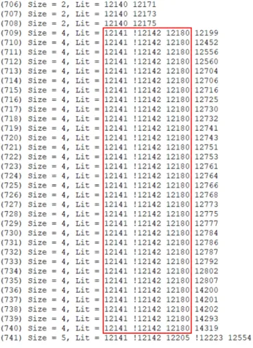
6s288r is a classic example depicted in Figure 3.1. For most of the clauses in the figure, they all share a common part (enclosed in the red box) and only differ by one literal. Intuitively, if the common part is added during the process, we may save the effort to prove those clauses. However, at first glance, this kind of pattern seems to tell

(29)

us that it is a reachable state that hinders the blocking since a cube can be blocked only if all the states in it are unreachable. That is, in cube (12141, !12142, 12180), a smaller cube or even a minterm may be reachable so that PDR must avoid to block those states.

Figure 3.1: 36 blocked cubes out of the 889 ones in the inductive invariant set of 6s288r.

The number in the parentheses means the index. The numbers after ”Lit” are the IDs of latch variable. Exclamation mark means the literal is complement.

Surprisingly, by directly set this cube to be the property, we easily prove that the whole cube is unreachable by PDR itself. It only costs five clauses for the inductive invariant set within tens of milliseconds. Now the question is why PDR struggles to block the bad states spreading around the cube by so many clauses instead of only one. (For convenience, we extend the term bad to describe any state that leads to the violation eventually since the result is equivalent.) Here we restate the seemingly reachable state as hard-to-block state and provide a possible reason in the next paragraph.

(30)

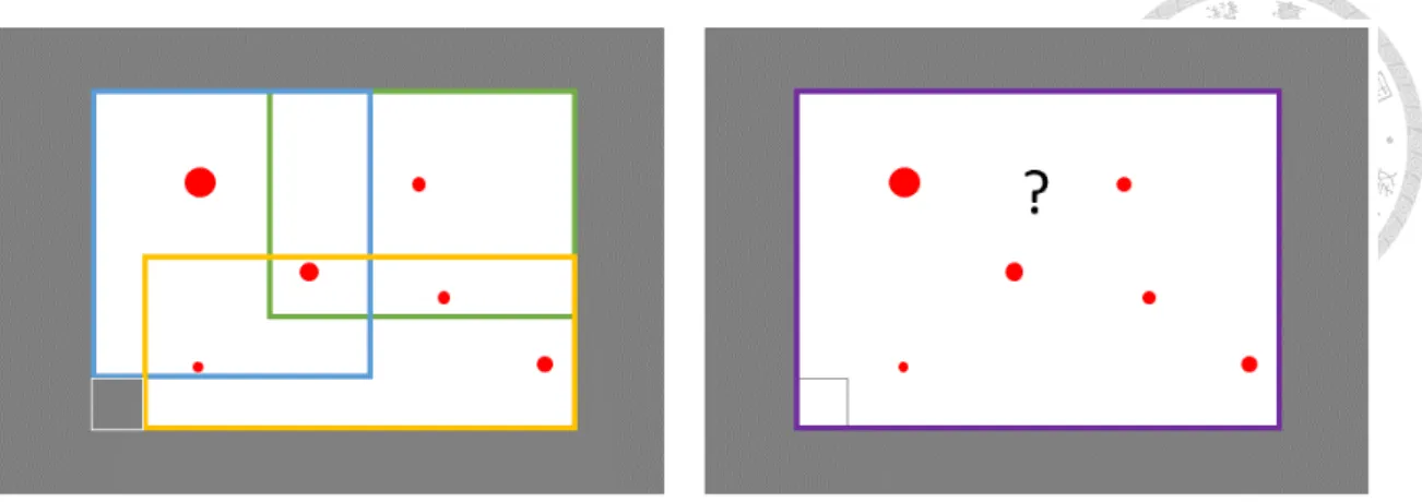
Figure 3.2: The depiction of the similar clause problem. The largest rectangle is the whole Boolean space. The middle rectangle means the cube as common part. There are many proof obligations (red spot) spreading around the cube. The gray area denotes that the state is reachable while the unreachable state in the white area has been blocked. The left subgraph illustrates what we observe. In order not to touch the lower-left cube, many blocking clauses are needed to tackle with the blocking. However, there is actually no such a state, as in the right subgraph. Why not just use a larger clause to represent it?

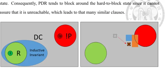
From the details introduced in the previous chapter, we know that every blocking clause is generated from a proof obligation. When excluding a proof obligation, we also block some other states by removing some literals of it in generalization process. A don’t-care state that is neither reachable nor bad is included in the final result if there is no proof obligation generalized to block it. Hence, the reachability depends on the appearance of proof obligation to a high degree. Corresponding to the name, property directed reachability, the reachability is computed by continuously eliminating the violation we want to prove. This scheme makes sense since we can just focus on the point of the problem. However, it sometimes prevents us to make better use of the don’t-care state. A state can be proven to be unreachable only if all the predecessors of it have been proven earlier. The hard-to-block state must be don’t-care since it will eventually be blocked if it is bad. In addition, we know that all the predecessors of it are don’t-care as well. If any of the predecessors is difficult to be blocked with the guide of the obtained proof obligation during the procedure, it probably remains reachable until the end. Therefore, PDR gives up for proving the unreachability of the hard-to-block state immediately without digging into the proof recursively just because it is not a bad

(31)

state. Consequently, PDR tends to block around the hard-to-block state since it cannot assure that it is unreachable, which leads to that many similar clauses.

Figure 3.3: The depiction of the reason for the similar clause problem. I, R, DC, !p,

!P means the initial state, the reachable states, the don’t-cares, the violation of property and the bad states, respectively. As the left subgraph, an inductive invariant set must include R and exclude !P. For the right subgraph, in order to block the bad states, two blocking clauses are involved (blue and orange). During generalization of them, they all want to include the brown states. However, the predecessor of the brown state has little connectivity to the property. Hence, PDR fails to prove their unreachability continually.

The inspiration for us is straightforward. If we can force the procedure to prove for some property more eagerly, we can make better use of the don’t-care states to find a more efficient and elegant clause representation. Hence we let the procedure solve the candidate separately if they find something weird, just as what we human beings do. If it really helps, the obtained information can be used to help the original main procedure.

Now, two phases are needed, including how to extract some patterns as predicate to solve and how to get information from it.

3.2 General Method and Correctness

As shown in Algorithm 5, the procedure is very simple. Given a predicate as any form to represent an assumed property, we start another PDR procedure with resource limit to work on it. Note that the procedure is activated without predicate solving to ensure the completeness. The resource limit is determined by the number of SAT query to indicate

(32)

expect to get from it. The procedure terminates if the answer is proved or the resource limit is used up. If the result is safe, we can collect the inductive invariant set. Otherwise, we can still get F_∞from it. For both case, we obtain an inductive set containing only clauses.

Then we directly merge it back to the F_∞of the original main procedure. The merge is trivial for two CNF since they basically do nothing except for some detailed checking like subsumption. After finishing the solving, PDR turns back to what it does previously and just go on without preparing anything for the correctness.

Algorithm 5: solvePredicate

Input: Predicate p^′ and the limit for SAT query L Output: None

1 Set SAT query limit to L

2 result← pdrMain(M, p^′)

3 if result = safe

4 ind← collectIndInv()

5 else // violated or unknown

6 ind← getInfF rame()

7 F_∞← F∞∧ ind

Theorem 3. Property directed reachability with predicate solving is sound.

P roof :

1. Property 1 and 5 are not related to this modification and hold trivially.

2. The merged set ind is composed of clauses and does not exclude the initial state so that Property 2 and 3 still hold.

3. By following the proof for Theorem 2, we show that Property 4 holds.

ind is inductive itself so that inductive relative to F_∞

F_∞(S)∧ ind(S) ∧ T r(S, S^′)→ ind(S) ∧ T r(S, S^′)→ ind(S^′)

Then it just means to add a set of clauses instead of only one.

The 5 properties still hold with the aid of predicate solving. The algorithm is sound. ■

(33)

3.3 Two Kinds of Predicate

We have introduced how to extract information from the predicate. It can be performed on predicate of general form. The rest problem is how to find an effective predicate. More precisely, we want to find the predicate within reasonable time compared to how much it gains for us. However, there should not be too much expectation on a single predicate, the improvement is probably established on a wide search. It may be good to spend less time for each checking to find a series of candidates no matter how useful they are.

In the following subsections, we provide two examples that can be easily identified during the solving process. Both of them are expressed by cube since the calculation only involves the essential components of PDR without doing further modification. It is worth mentioning that PDR can be seen as breaking the entire problem into small pieces without handling the whole timeframe at a time. What we do is to observe that whether PDR encounters obstacles during the last period of time. If it solves for a similar problem for a while, we can just make an assumption on that part to help PDR conquer it. Then we expect an improvement by smoothing the solving process with the aid of these local information.

3.3.1 Blocking Clause

As being the problem we mentioned, the first example is to eliminate the similar clauses.

Algorithm 6 illustrates the way to identify the candidates. We introduce two parameters to guide how to find the candidates, including Backtrack number (B) and Match number (M ). Generally, each frame can be associated with different value of these two numbers.

Backtrack number means how many clauses in the corresponding frame is backtracked to be considered from the last one. If the size of the frame is less than B, just take the whole frame into consideration. f indCommon can be composed of any rule to find the common part to solve. Here we just handle the case that there is only one difference of literal between two clauses just as what we encountered. The number of occurrence of each

(34)

common part is recorded in a structure. Match number serves as a threshold. The candidate is picked only when it occurs more than or equal to M times. Note that the returned set can contains no or more than one cube. In our implementation, this subroutine is placed after every addBlockedCube then solveP redicate is activated for every candidate.

Algorithm 6: findClsPredicate

Input: A blocked cube c and the frame k to block it Output: A set of cubes

Data: A map candM ap from cube to unsigned number

1 size← |Fk|

2 B, M← getP aram(k)

3 n← min(size, B)

4 for c^′ in the last n cubes∈ Fk 5 common← findCommon(c, c^′)

6 if common̸= N^ULL

7 // By default, every cube maps to 0

8 candM ap[common]← candMap[common] + 1

9 return{c^′| candMap[c^′]≥ M}

Figure 3.4: An example for clause-based predicate. After adding the cube to its corresponding frame, only the last several cubes are considered to find the common part.

There may be multiple common parts, but only the ones occurring more than the threshold are picked.

(35)

3.3.2 Proof Obligation

For some cases, all the proof obligations for them share a common part. The common part here means the intersection of literals and we collect them to be a cube. Firstly, we set the negation of the cube as the initial state and keep the original property. For some cases, it is still safe, which means all of the bad states really locate in that cube. However, if we keep the initial state and set the cube as the property. They are easily proved to be violated, that is, not all of the reachable states locate in the negation of that cube. In Figure 3.5, we show the possible distribution of reachable and bad states.

Figure 3.5: The possible distribution of reachable and bad states for similar obligation problem. The lower-right rectangle means the cube of shared literals. The difficulty of this kind of problem is probably to show that the reachable states do not intersect with the bad states in this cube.

The global constraint is too loose to represent a useful information. It turns out that local information makes sense again. We present the procedure to collect the common part in Algorithm 7. A set of cube and a counter are kept globally since the result becomes available after a period of accumulation. At each time of collection, the counter increases by one to indicate that one more proof obligation is considered. Furthermore, we continuously compute the common part by the given obligation. However, we do not return predicate in this subroutine. This is not like the case for blocking clause that the candidate can be produced at every query to find predicate. Algorithm 8 demonstrate when and how to use obligation as predicate. The collection is performed when the proof

(36)

check the availability of predicate only if the obligation can be reached from the previous frame. We introduce a parameter called Obligation threshold (T ) here. If the cumulative number of obligations exceeds T , we collect the common part as a cube to be predicate if it is not empty. After checking the predicate, we reset the cumulative number and continue to block cube recursively.

Algorithm 7: findOblPredicate Input: A proofobligation o Output: None

Data: A set of literals common and an unsigned number numObl (Keep globally. By default, common =∅, numObl = 0)

1 numObl← numObl + 1

2 if numObl = 1

3 common← {l | l ∈ o}

4 else

5 common← common ∩ {l | l ∈ o}

Figure 3.6: An example for obligation-based predicate. At each beginning, all the literals are collected. During the process, intersection is performed to pick up the sharing literals.

At the time to check, if the cumulative number of obligations is still smaller than the threshold or there is no common part during this period, NULL is returned to disable the predicate solving; otherwise, a cube is returned as a predicate by gathering the rest literals.

(37)

Algorithm 8: recBlockCubesobl

Input: Cube badCube, the frame to block f Output: TRUEor FALSE

Data: An infinite array of set of cubes badArr

1 badArr[f ].add(badCube)

2 blockF rame← f

3 while blockF rame≤ f

4 if blockF rame = 0

5 return FALSE

6 targetCube← badArr[blockF rame].pop()

7 if not isBlocked(targetCube, blockF rame)

8 f indOblP redicate(targetCube)

9 preCube← checkReach(targetCube, blockF rame)

10 if preCube̸= N^ULL

11 badArr[blockF rame].add(targetCube)

12 blockF rame← blockF rame − 1

13 badArr[blockF rame].add(preCube)

14 if numObl≥ T

15 if not common.empty()

16 solveP redicate(toCube(common), L)

17 numObl← 0

18 else

19 addBlockedCube(generalize(targetCube, blockF rame))

20 if blockF rame < f

21 badArr[blockF rame + 1].add(targetCube)

22 if badArr[blockF rame].empty()

23 blockF rame← blockF rame + 1

24 return TRUE

(38)

3.3.3 Recap for 6s288r

In this subsection, we provide more details about 6s288r that serves as the example in Section 3.1 by the following figures. Although the real cause of this phenomenon still needs to be verified, these facts can be seen as clues for the final answer.

Figure 3.7: The proof obligations leading to the similar clauses. ”Check” means to block proof obligation in recBlockCubes and the number after ”frame” is the frame to block it. The blocked cube after ”UNSAT generalization” with the frame to add it is generated after successfully blocking a proof obligation. Note that the three examples are not under computation in a row, we just collect them together to present. Most of these proof obligations have bad depth equal to 8, and the rest small portion with 14 or 16. We know that these proof obligations locate in the 8th steps from !p. Furthermore, they all share a common part but different for the rest literals and even the length. We then guess that these proof obligations describe a similar scheme of possible violation. Limited by the reachability, PDR has difficulty blocking them all at a time.

(39)

Figure 3.8: The cone of 12141 !12142 12180. The variables (latch ID) after the colons are the respective cone of these three latches. A variable is in the cone iff the function of the latch is dependent of this variable. We can see that the cone of these three latches are similar, and the distribution of variables locates in a range smaller than 100 (12126∼ 12214).

Figure 3.9: The cone of the literal along with 12141 !12142 12180 in Figure 3.1. We just take 6 out of them to present. These latches are not necessarily related to 12141, 12142 and 12180, but they all depend on itself.

We have not found a strong evidence to show the cause of the similar clause problem.

We just make a guess based on these observations. In the following three figures, the reason that the clauses with 12141 !12142 12180 can be added is by the help of the clauses added before them. This is because the proof obligation generates the others so that we know it is not able to be blocked initially. For the three situations, the first added clause cannot be enlarged anymore. (Become Tautology, 12142 12180, !12126 !12134) We then guess that it is this limit that prevents PDR from removing the literal during generalization.

(40)

Figure 3.10: Blocking procedure for the similar clauses (1). The actions of blocking in these three figures take place in a row. Although in the presented situations, the last literals are the same (12716, 12766, 12743), actually there exists the case that does not follow this regularity. In this figure, the two blocking clauses are generated by one proof obligation at different frames.

Figure 3.11: Blocking procedure for the similar clauses (2). In this figure, the above two proof obligations are the same, and the third is the one generating it.

(41)

Figure 3.12: Blocking procedure for the similar clauses (3). In this figure, the upper proof obligation is generated by the lower one. That is, the second generates the first and the third generates the second.

We further make an informal conclusion here. For the case of 6s288r in this subsection, we know that there also exists regularity for the proof obligations. However, since the proof obligation related to this phenomenon does not appear in a row, we cannot get the common part by our checking method. On the other hand, after the blocking clause is added to the frame, we can observe the similarity from the clauses. Hence, sometimes these two kinds of predicate may be complementary for each other, but it still needs more modification to achieve a balance of cooperation.

(42)

Chapter 4 Implementation

In this chapter, we describe our model checking environment called ”Ia2b” briefly. We also introduce what optimizations are applied in the engine to make it more efficient.

4.1 The Model Checking Environment

For the research of this thesis, we implement a model checking environment called

”Ia2b”. It contains compilation environment, command line interface, AIG network structure, simple simplification methods and various model checking algorithms.

The compilation is very trivial that every sub-directory under the source directory serves a module. Every compilation unit in each module is compiled to an object file, then all the object files are gathered to form a static library. The dependency simply follows the hierarchy mentioned above.

A basic command line interface is provided to facilitate the use of model checking engine. It is not as powerful as the mature shells like Bash at all, but is enough for the experiment. In addition to the fundamental string manipulation, the auto completion for command token, option and name of files is available. We support variadic length of tokens for command. Furthermore, for each token, the corresponding utility will be invoked as long as the mandatory part of it is satisfied. That is, we do not need to type full string for the command. Moreover, signal handling is also supported. For example,

(43)

the command line will be arranged to the settings at the time the process is paused when restoring, or the position of the characters will be changed to follow the window size.

We only support And Inverter Graph (AIG) for the network structure to follow the benchmarks in HWMCC [26, 27]. That is, there are only five gate types in the network, including constant zero (Const0), primary input (PI), latch (Latch), primary output (PO), and AND gate (And). In addition, some basic logic minimization methods like [28, 29, 30] are included though they are not activated in the experiment.

In addition to PDR, another engine like BMC, IND and IMC are also implemented, but we will not focus on them here. The implementation of our PDR basically follows the description in [18]. We simply introduce some main data structures we use and the optimization is presented in the next section. Figure 4.1 depicts the memory arrangement of cube for PDR. This structure is used by both proof obligation and blocking clause. All the information is collected to store in a chunk of memory that is continuous. Bad depth and the previous proof obligation are only meaningful for proof obligation and are wastes for blocking clause. Signature for subsumption is the method proposed by [31].

There are two Boolean flags for miscellaneous purpose. Reference count is to record how many places hold the address of this chunk of memory. Once the counter decreases to be zero, the occupied memory should be released since no one can access it anymore.

Number of literals is kept in order to define the boundary of the literals after it. This array-like memory allocation for a series of literals comes from MiniSAT [6]. However, we do not explicitly employ memory management to allocate all the cubes together.

Instead, we just use the built-in allocation utility from C++ to request and return the memory. Besides, the structure for the frames is simply vector of vector of cube. F_∞is always kept to be the last element. This linear storage is convenient for iteration and is actually not so inefficient for deletion of subsumed clauses.

(44)

Figure 4.1: The memory arrangement for cube of PDR.

4.2 Optimization and Other Things We Tried

In this section, we introduce different implementation techniques for every part of PDR and discuss about their efficiency.

4.2.1 Subsumption

Although subsumption checking is a very simple task, but it is performed for a great number of times throughout the process. We need to check subsumption for every blocking clause before either blocking a proof obligation or adding a new blocking clause. That is, as the number of blocking clause grows, the overhead of subsumption increases dramatically. The following are a series of methods to check if c₁subsumes c₂. 1. The most trivial method is to iterate over c₂for every literal in c₁to check if it is in

c₂. The complexity is|c1|×|c2|.

2. For the rest methods, we use some rules to do early break on the checking. The use of signature is proposed by [31] to record the existence of a literal to a specific bit in a number. Before doing the detailed checking, we first check the sizes and the signatures to filter the apparently failed cases. For the cubes, we maintain that they are sorted. If we find that a literal in c₁is at a position of c₂, the literals of c₁ behind that must locate after that position in c₂ if the subsumption holds. This results in a linear checking procedure since we just need to iterate over c₂for one time without going back again. The complexity is |c1| + |c2| and we adopt this method in our implementation.

(45)

3. Consider that the size of proof obligation is often much larger than that of blocking clause. We can use binary search to check if a literal in c₁ is in c₂ since we assure the cube is sorted. The complexity becomes|c1|×log|c2|.

4. As in [31], the subsumption checking can be generalized to be a self-subsumption one. However, this introduces an overhead that cannot be ignored. This is because there are more literals being processed by self-subsumption checking due to its looser criteria. When the subsumption is sure to fail, they are still possible to be self-subsumption. Since we just need pure subsumption here, so the general process for self-subsumption is discarded.

4.2.2 Ternary Simulation

Ternary simulation plays an important role for efficiency of PDR because of not only the effect to maximize the proof obligation but also the runtime taken by it. Hence, it is important to reduce the overhead of it without sacrificing the quality. In the following, we introduce several kinds of method and the last two have not been verified by implementation yet.

1. The ternary value is encoded by two bits and the transition of an AND gate follows the method in MiniSAT 2.2.0 [32]. We encode the result in a magic number in advance and use bit shift to get the answer based on the two inputs. This is actually equivalent to a 3×3 look-up table. For the most straightforward method, we do the normal simulation in the topological order. We collect the cone related to the target first and the latches not in the cone are trivially don’t-care. Then we do constant propagation based on the value of primary inputs since we will not modify these values during the process. By doing these two steps, we can reduce the number of gates to simulate massively.

2. Since we only modify the value of one latch at a time, the influence may not transit

(46)

gate in need. An event is that we need to re-simulate a gate due to the change of any of its inputs. We still need to collect the cone of target to eliminate the latches trivially don’t-care and to prevent the event from spreading out of the cone. We adopt this scheme thanks to the balance of runtime and quality.

3. Backward simulation is very fast since its complexity is only linear to the size of the cone. First we assign the value of every gate in the cone by performing simulation once or extracting from the SAT solver. Then we backward mark the set of don’t- care based on the following rules from the target.

(a) If the output is 1, both of the inputs must be also 1s and should be kept.

(b) If the output is 0 and the input combinations is either (0, 1) or (1, 0), we can keep the value 0 and mark the other input with value 1 to be don’t-care.

(c) If the output is 0 and both of the inputs are also 0s, we can pick one of the inputs to keep the value and mark the other to be don’t-care.

Note that the mark of don’t-care is dominated if the value is mandatory for another part of circuit. After one traversal, we can directly remove the latches that are really don’t-care.

4. The cube in the original PDR can only contain state variables. This scheme sometimes increases the number of blocking clause like representing XOR gate.

An idea is to use the internal signal of the circuit in the cube to represent the state.

This does not mean to find a cut for representation, but to use different set of gates in different cubes. Note that the used gate cannot be related to any primary input, that is, the cone of it can only contain latches. If it does contain any primary input, the semantics for state representation is broken.

5. The last method uses SAT instead of ternary simulation. First we make an assumption on the negation of the target. We then make assumptions on the assignment of primary inputs and latches. The query must be UNSAT so that we