財務金融研究

國立臺灣大學管理學院國際企業研究所 博士論文

Department of International Business College of Management

National Taiwan University Doctoral Thesis

財務金融研究

Essays in Finance

周盈吟 Ying-Yin Chou

指導教授：洪茂蔚 博士

Advisor: Mao-Wei Hung, Ph.D.

中華民國 100 年 7 月

July, 2011

誌謝

在國企所博士班六年的學習過程，隨著論文的付梓，即將劃上句點，這段時 間以來的點點滴滴，有回憶，有不捨；回憶之情將在我的懷中日漸晶瑩光耀，不 捨之心將使我的人生成就勇氣。

本論文能順利完成，幸蒙洪教授茂蔚的指導與教誨，對於研究的方向、觀念 的啟迪、架構的匡正、資料的提供與求學的態度逐一斧正與細細關懷，於此獻上 最深的敬意與謝意。論文口試期間，承蒙口試委員的鼓勵與疏漏處之指正，使得 本論文更臻完備，在此謹深致謝忱。

在博士班修業期間，感謝韓教授南偉、郭教授家豪等諸位老師在課業知識的 傳授。同窗伙伴六年來的切磋討論與鼓勵，獲益良多，永難忘懷。

最後，特將本文獻給我最敬愛的母親，感謝您無怨無悔的養育與無時無刻的 關懷照顧，還有父親及大哥、小妹在經濟上與精神上的支持，讓我能專注於課業 研究中，願以此與家人共享。

感謝所有人，讓我這一路走來平安順利。今後希望能有更多機會將所學貢獻 於社會，並回饋給更多需要幫助的人們。

盈吟 謹誌於 台灣大學國際企業研究所博士班 中華民國一百年七月

中文摘要

這篇論文主要是探討抗通膨債券的定價與投資者消費投資組合的最佳化解。在此 篇論文的第一部分，我們在通膨率有隨機波動度下，得到一個美國抗通膨債券(TIPS)

的解析解。在實證上，我們利用美國市場上的二十九支 TIPS 價格，求出在 2000

年一月到2009 年十月期間，模型的未知參數和通膨利差。實證結果顯示，忽略隱

含選擇權將導致通膨利差的高估。平均來說，高估的部分大概是 0.82%。實證結果 同時顯示，所得出的最小的利差發生在 2009 年一月附近，此時間點為本文探討期 間發生最嚴重的通貨緊縮時點。在此篇論文的第二部分，我們解一個跨期消費投 資組合問題當市場存在通膨風險時。投資人為了對抗通膨風險，會選擇持有抗通 膨債券。本文說明，名目利率和通膨率如何影響最佳化消費財富的比例與跨期替 代彈性有關。消費財富的比例不完全受到實質利率影響，同時也與名目利率和通 膨率有關。最後，利用美國市場資料對模型做一個補正，結果顯示，積極型的投 資者會想要擁有較多的名目債券以賺取通膨風險貼水，而保守型的投資者會持有 較多的通膨債券以規避通膨風險。

關鍵字: 隨機波動度，美國抗通膨債券，隱含選擇權，通膨風險，指數型債券，

投資組合選擇，跨期替代彈性

英文摘要

The purpose of this thesis is to price the inflation indexed securities and solve for an inter-temporal portfolio consumption choice problem under inflation. In the first part of this thesis, a diffusion model for inflation rates with stochastic volatility is proposed, and closed-form solutions are derived for treasury inflation protected securities (TIPS).

Empirically, our model with 29 TIPS, treasury constant maturity rates and reference CPI numbers in the U.S. market was used to derive the unknown parameters and spreads during January 2000 to October 2009. Empirical results show that an over-estimated spread is induced by ignoring the embedded option in TIPS. The average difference between the distorted estimate and actual value is about 0.82%. The minimum spread occurred around Jan. 2009 while the CPI-U decreased drastically. In the second part of this thesis, we solve for an inter-temporal portfolio consumption choice problem under inflation. The inclusion of the inflation-indexed bonds in the investor’s portfolio provides an opportunity to perfectly hedge against the inflation risk, while the hedging demand of the nominal bonds would be crowded out in proportion to the demand of the indexed bonds. The direction in which the interest rate and the inflation rate affect the optimal consumption-wealth ratio relies on the elasticity of inter-temporal substitution of the investor. The consumption wealth ratio is not completely determined by the real interest rate, it also depends on the nominal levels of

the interest rate and the inflation rate. The capital market is calibrated to U.S. stock, bond, and inflation data. The optimal weights show that aggressive investors hold more nominal bonds to earn the inflation risk premium, and conservative ones concentrate on indexed bonds to hedge against the inflation risk.

Key words: Stochastic volatility, TIPS, Embedded option, Inflation Risk, Indexed Bond, Dynamic Portfolio Choice, Elasticity of Inter-temporal Substitution

目 錄

口試委員會審定書………i

誌謝 ……….…………...….ii

中文摘要 ………...….iii

英文摘要 ………...….iv

Chapter 1 Treasury Inflation Protected Securities pricing under the Heath-Jarrow- Morton model with Stochastic Volatility……….…...1

1.1 Introduction………...1

1.2 Model………....3

1.3 Pricing TIPS ………..…...4

1.4 Numerical examples ………...10

1.5 Empirical analysis………...12

1.5.1 Data description………...12

1.5.2 Empirical result………...13

1.6 Conclusion………..19

1.7 Appendices………...20

Chapter 2 Optimal Portfolio-Consumption Choice under Stochastic Inflation with Nominal and Indexed Bonds………...37

2.1 Introduction………37

2.2 The Economy………...42

2.2.1 The Dynamics of Price Level and Expected Inflation………...43

2.2.2 The Bond Market………...45

2.2.3 The Optimization Problem………...48

2.3 Results………...51

2.3.1 The Approximate Solution with Log-Linearization...52

2.3.2 The Optimal Policies………...53

2.3.3 Dynamics of Nominal and Real Consumptions...60

2.4 Model Calibration………...63

2.4.1 Calibration of model parameters…………...63

2.4.2 Optimal portfolio strategy………...65

2.5 Conclusions……….………...67

Reference……….……….…...77

圖目錄

Figure……….…..29 Chapter 1

Figure 1 Common nominal and real term structures……….…..29 Figure 2 Coupon rates of TIPS……….………...30 Figure 3 Embedded options in TIPS……….……….…..31 Figure 4 Over-estimated spreads between nominal and real rates induced by ignoring

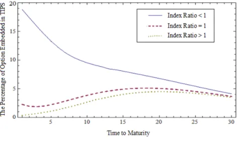
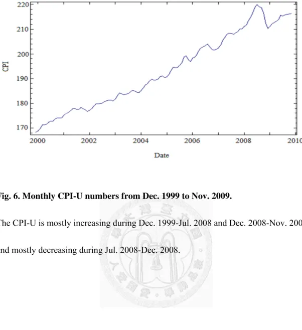
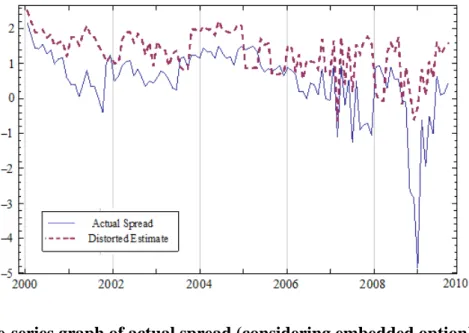
embedded options in TIPS……….……….…...32 Figure 5 The percentages of options embedded in TIPS of different index ratio...33 Figure 6 Monthly CPI-U numbers from Dec. 1999 to Nov. 2009…...……...…...34 Figure 7 The time-series graph of actual spread (considering embedded option) versus

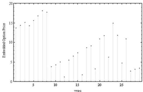
the distorted estimates (without considering embedded option)…...35 Figure 8 The estimated price of option embedded in each TIPS………...36

表目錄

Table………...…….26

Chapter 1 Table 1 The TIPS data set starts from January, 2000 to October, 2009.26 ……..…....26

Table 2 Values of the estimated parameters and their standard errors…...…...27

Table 3 The average prices and percentages of options embedded in TIPS of various maturity periods…….………..………..………..…...28

Chapter 2 Table 1 Estimates of Model Parameters……….……...….70

Table 2 Estimates of Model Parameters……….………...….72

Table 3 Optimal portfolio strategy……….……...…….73

Table 4 Optimal portfolio strategy……….…...……….74

Table 5 Optimal portfolio strategy……….………...….75

Table 6 Optimal portfolio strategy……….………....76

Chapter 1

Treasury Inflation Protected Securities Pricing

under the Heath- Jarrow-Morton model with Stochastic Volatility 1.1 Introduction

Since January 1997, the treasury inflation protected securities, or TIPS, created by the U.S. treasury to help investors manage inflation risk, have been issued regularly.

Principals of TIPS are adjusted periodically to keep pace with the rate of inflation, measured by the consumer price index for all urban consumers (CPI-U). Investors receive semi-annual coupon payments based on a fixed semi-annual coupon rate applied to the inflation-adjusted principal. At maturity, if inflation has increased the value of the principal, investors receive the higher value. If deflation has decreased the value, investors still receive the original face amount of the security. The redemption valuation at maturity is recognized as an embedded option in TIPS.

Fischer (1975) first analyzed the demand for index bonds. Unlike traditional treasury bonds, investors in TIPS are guaranteed by the government a specific rate of return and a specific purchasing power of the principal above inflation. According to the estimates of the treasury department, the outstanding volume of TIPS has risen from about $15 billion in 1997 to about $413 billion by late 2006, and trading of TIPS among primary securities dealers has risen from a daily average of $1 billion in early 1998 to

approximately $8 billion by late 2006 due to their built-in inflation protection.

Yields calculated from prices of TIPS are usually denoted as approximations of inflation-adjusted or real interest rates. That information, together with yields on traditional, nominal-treasury securities, is often used to provide implicit indications of general agreement of medium-term to long-term expectations of inflation by the bond market. However, the fact that the long-term inflation expectation from the survey has almost always been higher than that computed from the spread between nominal and TIPS yields (called term premium) suggests that measure is distorted. As a measure of expected inflation, the spread between nominal- and indexed-treasuries could be distorted by inflation uncertainty, risk aversion, and the probability of deflation.

Like Melino and Turnbull (1990), Frachot (1995), or Bakshi and Cao, we propose a much more general and flexible pricing model for TIPS with embedded options which allows for consideration of stochastic volatility and correlations among inflation rates, nominal forward rates, real forward rates, and volatility variants. This aids in more accurately capturing the distribution properties of inflation. However, due to the long maturity property of TIPS, fitting the current term structure is an important consideration for practitioners. Jarrow and Yildirim (2003) applied the term structure model introduced by Heath, Jarrow, and Morton (HJM) (1992) to both nominal and real rates. Options embedded in TIPS also have long maturity and are very different from

ordinary options. Unlike an ordinary option, whose value always increases with maturity, the relation between the TIPS-embedded option and maturity is much more complex. The relationship depends on the term structures of real and nominal forward rates and the reference CPI-U on the issue date. This article provides the theoretical and empirical basis of TIPS for pricing in the stochastic volatility framework.

The remainder of this article is as follows: Section 2 describes the model and its assumptions. Section 3 introduces the general valuation framework and presents closed-form solutions of TIPS. Section 4 investigates the properties of TIPS and embedded options using numerical examples. Section 5 reports the empirical analysis based on the U.S. market data. Conclusions are given in Section 6.

1.2 Model

The HJM model was applied to TIPS in order to fit best the current term structure, which is the first-order requirement for practitioners while pricing high interest-rate-sensitive derivatives. As presented in Duffie, Pan, and Singleton (2000), we assumed that, at timet, the data-generating processes of the inflation index, with its stochastic variance component, , the nominal-

), (t I )

(t

Y T -maturity forward rate,

, and the real )

, ( Tt

F_n T-maturity forward rate, F_r( Tt, ), are calculated as follows:

() ( ) ( ) () ()

) (

)

( t dt dW t dW t Y t dW t

t I

t dI

I r

Ir n

In

I   

   , (1)

) ( ) ( ))

( (

)

(t Y t dt Y t dW t

dY  _Y _{Y Y} , (2)

dF_n(t,T)_n(t,T)dt_n(t,T)dW_n(t), (3)

) ( ) , ( )

, ( ) ,

(t T t T dt t T dW t

dF_r _r _{r r} , (4)

where , , , and describe standard Brownian motions with covariance:

) (t

W_I W_Y(t) dW Cov _I

) (t

W_n W_r(t) dt dW_Y)_IY ,

( , Cov(dW_n,dW_r)_nrdt , , ,

0 ) ,

(dW_I dW_n  Cov

0 )

I,dW dW (

Cov _r Cov(dW_Y,dW_n)0 , and . Structural

parameters

0 ) dWr

, (dW_Y Cov

, _Y, and _Y represent the long-run mean, the speed of adjustment, and

the volatility of the stochastic variance component, respectively. The timet, price of a nominal (real) zero-coupon bond maturing at timeT, in dollars (CPI-U units), is given by Eq. (5).



_ 

 ^T

t k

k t T F t s ds

V ( , ) exp ( , ) , k

 

The nominal (real) money market account is defined as

 _ 

 ^T

t k

k t T r s ds

B (, ) exp ( ) , k

 

where r_k(t) is the spot rate and r_k(t)F_k(t,t) . The instantaneous covariance rate--between inflation rates and nominal (real) rates--is given by _n(t,T)





(_r(t,T)





1.3 Pricing TIPS

If true processes are given by Eqs. (1)-(4), the processes under the risk-neutral measure,

Q, defined by (W_I^*(t), W_Y^*(t), W_n^*(t), W_r^*(t)) are given by Eqs. (7)-(10),





t I

t dI

I r

Ir n

In

I() () () ( ) ()

) (

)

(        

) ( ) ( ) ( )

( ^{* *}

* t dW t Y t dW t

dW_{n Ir r I}

In  

  , (7)





)

(t Y t dt Y t dW^* t

dY  _Y _Y _{Y Y} , (8)

dF_n(t,T)









,

(t T t T t T t dt t T dW^* t

dF_r  _r _r _r _{r r} , (10)





k , ,

where _k(t) is the market price of W_k(t) for  and _Y is the volatility risk premium. After adopting the assumption that _Y Y(t) (Bates (1996)), Eq. (8) can be rewritten as

) ( ) ( ))

( (

)

(t Y t dt Y t dW^* t

dY   _{Y Y} , (11)

where  _Y . A proposition is presented that states the necessary and sufficient conditions for bond price evolution to guarantee that arbitrage does not exist.

Proposition I: Arbitrage free term structures ( , ) / (0, )

n n

V t T B t , , and are Q-martingale if

and only if

( ) ( , ) / (0, )_{r n}

I t V t T B t I t B( ) (0, ) / (0, )_r t B_n t



 

 ^{(, )}



) ,

(t T t T ^T t u du _n t

t n

n

n   

 (12)



   

 r



r t T  t T  t u du  t   

 ( , ) ( , ) (, ) ( ) (13)

) ( ) ( ) ( )

( )

( ) ( )

(t r_n t r_r t _{In n} t _{Ir r} t Y t _I t

I     

      (14)

Proof: See Appendix A.

From Eqs. (7) and (9)-(11), and Proposition I, the following equations are derived under the risk-neutral measure, Q:





) (

)

( _{* * *}

t dW t Y t dW t

dW dt

t r t t r

I t dI

I r

Ir n

In r

n    

   , (15)





)

(t Y t dt Y t dW^* t

dY   _{Y Y} , (16)

( ) (, ) ( ) )

, (

) ,

( _*

t dW T t a dt t T r

t V

T t dV

n n

n n

n   , (17)

 



T t V

T t dV

r Ir nr In r

r

r ( ) ( , )

) , (

) ,

(     



where ak(t,T)^



 

) , (t 

V_n^T I_V^T(t,) I_r^T(t) )

, (t

Vn , I(t)V_r(t,), and with respect to as defined by

) , 0 ( t ) ( Bt I _r )

, ( Tt

V_n V_n^T(t,)V_n(t,) V_n(t,T), I_V^T(t,)I(t)V_r(t,) V_n( Tt, ), and

 ) (t

I^T_r I(t)B_r(0,t) V_n(t,T), where T  . Other forward prices are defined in a similar manner. Next, is determined under which , , and

are martingale.

QT V_n^T(t,) I_V^T(t,) I_r^T(t)

Proposition II: Martingales under measure Q^T ( , ) / ( , )

n n

V t V t T , I t V t( ) ( , ) / ( , )_r  V t T_n , and are martingale under

defined by { , , , }, where ,

, , and .

( ) (0, )/ ( , )_{r n} I t B t V t T

)

T(t

n W_r^T(t)

ds W_r^T(t)W_r^* QT

) ( )

(t W^* t W_Y^T  _Y

) (t

W_I^T W_Y^T(t)





 _n ^t _n

T

n t W t a

W 0

*( ) )

(

W T )

) ( )

(t W^* t W_I^T  _I



nr a sT ds

0 ( , )

 s,

( (t)

Proof: See Appendix B.

Let E_t^Q and E_t^T denote the conditional-expectation operators at time t under

the risk-neutral measure and the forward-neutral measure , respectively. Kijima and Muromachi (2001) demonstrated that, if the relative price of a risky asset is a martingale under the risk-neutral measureQ, and its forward price is also a martingale

under the forward-neutral measure, , then

Q Q^T

) (t S

QT



 



 





 





) , (

) ) (

, 0 ( ) 0 ) (

, 0 (

) (

0

0 V T T

T E C

T V T C

B T E C

n T n

n

Q (19)

where C(t) is the time t price of a European derivative maturing at time T written on S(t).

Consider a European call option issued against the inflation index with a strike price of K index units and maturity dateT . Because the index is denominated in units of dollars per CPI-U, each unit of the option was assumed to be written on one CPI-U unit. Therefore, the time T payoff to the option, in dollars, is equivalent to

. The present value of this option can be formulated as





maxI T K





 



 

 max ( ) ,0

) , 0 ( ) 1

,

( ₀ I T K

T E B

K T C

n

Q



Instead of solving Eq. (20) under the risk-neutral measure, it was solved by transforming into the forward-neutral measure. BecauseV_r(T,T)1, Eq. (20) can be written as:

 



 



 max ( ) ,0 )

, 0 (

1

0 I T K

T E B

n

Q

 



 



 

 max ( ) ( , ) ,0

) , 0 (

1

0 I T V T T K

T

E B _r

n

Q . (21)

Combining Proposition I and Proposition II, and Eq. (19), yields

 



 











 





 



  ,0

) , (

) , ( ) max ( )

, 0 ( 0

, ) , ( ) ( )max , 0 (

1

0

0 K

T T V

T T V T E I

T V K

T T V T T I

E B

n T r

n r

n

Q . (22)

Proposition III is provided for deriving the formula of C(T,K).

Proposition III.



The present value of ^m



measure, , is given by

ax ( ) ( , ) / ( , )I T V T T V T T_{r n} K,0 QT



 











  ,0

) , (

) , ( ) max (

0 K

T T V

T T V T E I

n

T r ( )

) , 0 (

) , 0 ( ) 0

( i v

T V

T V I

n

r   

 K( v ), (23)

where ( )

IV



 is defined by



(_IV)











 



 



 



 



 





0

) , 0 (

) , 0 ( ) 0 ln ( ) 0 ( )

; ( ) , ,

; , 0 ( exp 1 Im

2

1 dv

v

T KV

T V iv I

Y T B T T T A

n r I

IV V



 ^.

Proof: See Appendix C.

Combining Eqs. (20)-(22) with Proposition III, generates Eq. (24).

( , )

C T K I(0)V_r(0,T)(iv)KV_n(0,T)(v). (24) Pricing TIPS is performed in much the same way as for a conventional bond with the addition of mechanisms for inflation adjustment and redemption valuation at maturity.

The present value (in dollars) of a TIPS coupon-bearing bond issued at time t₀( 0),

C

with a coupon payment of , the face value of F, and the maturity of T, is given by

0 0

1 0 0

( ) ( )

(0) ,1

(0, ) ( ) _n(0,

C F

B t ) ( )

n Q i Q n

TIPS

i n i n

I t I t

B E E Max

B t I t I t



 

  

  

 

 

 

    



where is the t_i i-th coupon payment date and t_n T. The value for redemption at maturity is the larger of either the original issue par value or the cumulative inflation-adjusted par value. When investors are concerned about the chance of deflation, the embedded option of TIPS at redemption may be very valuable. Eq. (25) can be

written in another form:

 





 







 n

i n i

i Q

TIPS B t

t E I

t I B C

1

0

0 (0, )

) ( )

) ( 0

( )

) , 0 (

0 ), ( ) ( )

(

0 0

0

T t FV

B

t I E T

t I

F

n n

Q 



 



 

, 0

n( I

Max . (26)

In which E₀^Q











0)

 )





 n

i r i

n

TIPS I t

t I CV T

FV B

1 (

0 ) ( , 0 ( )

, 0 ( )

0 (

) ) (

( ) 0 ) ( , 0 (

0

v t i

I T I

FV_r    FV_n(0,T)(v). (27)

by incorporating Eq. (24). After defining(x)1(x), Eq. (27) can be written as

1 0 0

(0) ( )

I I

T I t

(0) (0, ) (0) (0, )

( )

n

TIPS r i r

i

B CV t FV

 I t





) ) (

( ) 0 ) ( , 0 (

0

v t i

I T I

FV_r   

 FV ,_n(0T)(v). (28)

If we ignore the embedded option in TIPS, the final two terms in Eq. (28) will also be ignored; subsequently, the price of TIPS can be completely determined by the term structure of real forward rates. However, the existence of the embedded option at

redemption makes it possible for nominal forward rates and stochastic volatility to play an important role in determining the price of TIPS.

Given the market prices of TIPS, using the pricing formula of TIPS without the embedded option at redemption may result in under estimation of the real interest rate.

This approach may induce over estimation of the spread between nominal and real interest rates. If the over-estimated spread is treated as a measure of future inflation rates, an over-estimated future inflation rate will result. Historically, the market has generated an over-estimated future inflation rate from the yield spread between treasury bonds and TIPS.

If issuing TIPS at the face value in the beginning (t₀ 0), the coupon rate, , can be determined by

c





  _n

i

i r n

t V

I I T C T c V

1

) , 0 (

) 0 ( )) 0 ( , ( ) , 0 (

1 . (29)

1.4 Numerical examples

According to Jarrow and Yildirim (2003), we specify

 





) ,

( q T t

q T p

t

a _k

k k

k     , ^k

 

. Although the treasury yield curve has exhibited different shapes during the past several decades, Fig. 1 provides the common shape of the nominal term structure

0.011 pr  0.013

q_r 

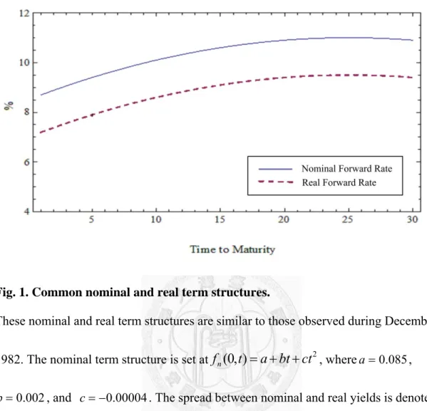
(similar to that observed during December 1982). The nominal term structure is set to be f_n(0,t)abtct², wherea0.085,b0.002 andc 0.00004.

For simplicity, the spread between nominal and real yields is assumed to be deterministic, and is denoted as s(t). After specifying s t( ) 1.5% , the real term structure can be obtained by f_r( t0, ) f_n( t0, )s(t). Next, we set , ,

,

0 0

t F 1

, _In 0, _Ir 0, _IY -0.512, and

Y 0.01

, ,

(0) 0.03  0.0005

Y  6.02

0.110

nr 

( ) s t 

to investigate selected properties of TIPS and embedded options through numerical examples.

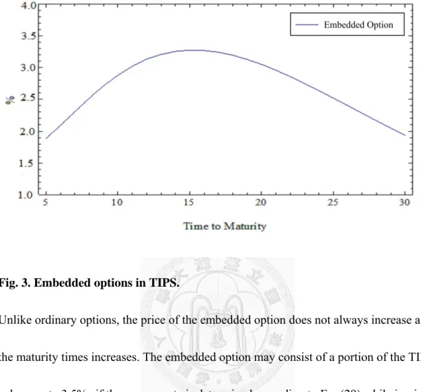
Fig. 2 depicts the relationship between the coupon rate of TIPS and the maturity according to the circumstance depicted in Fig. 1. In addition, Fig. 3 shows that the relationship between the embedded option price and the maturity, depending on both the nominal and real term structures, is not monotonously ascending. The embedded option may consist of a portion of the TIPS value. Its percentage can reach nearly 3.5% if the coupon rate is determined according to Eq. (29) while issuing TIPS at the start.

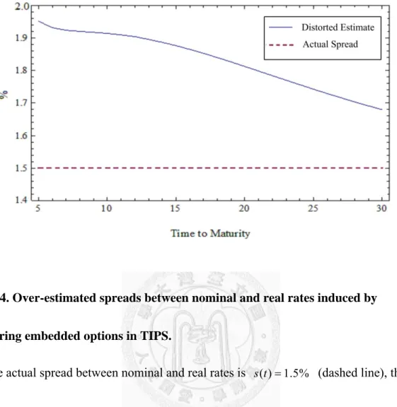
Fig. 4 shows that an over-estimated spread between nominal and real rates is induced by ignoring the embedded option in TIPS. If the actual spread between nominal and real rates is , the spread can be over estimated by 1.95% using TIPS with a 5-year maturity. The value is almost 1.3 times higher than the actual value. The shorter is the maturity period the larger is the distorted estimation.

1.5%

The embedded option may consist of a portion of the TIPS value, and its percentage may depend on the index ratio, . We set coupon rate to be 4%.

We vary the index ratio, and present the results in Fig. 5. The smaller is the index ratio, the larger is the percentage of option embedded in TIPS. The value of option embedded in the TIPS can reach nearly 19% of the TIPS value if the index ratio is smaller than 1, while that embedded in the TIPS can reach only 4.48% of the TIPS value if the index ratio is bigger than 1.

(0)/ ( )0

I I t

1.5 Empirical analysis

We organize this section into two parts: firstly, the data used in our empirical investigations are described. Secondly, the empirical results are shown.

1.5.1 Data description

The data used in our empirical investigation are daily market data from January 17, 2000 to October 23, 2009. There are three different data sets: nominal constant maturity treasury rate data, TIPS data and CPI-U data.

(i) Nominal constant maturity treasury rate data:

We obtain treasury constant maturity rates on all available U.S. treasury securities. A treasury constant maturity rate is defined to be the par yield of a government treasury security with a specified maturity. These rates are read from the yield curve at fixed maturities, currently 1, 3, and 6 months and 1, 2, 3, 5, 7, 10, 20, and 30 years.

(ii) TIPS data:

We obtain daily price on all available U.S. treasury inflation protected securities.

We choose 29 TIPS reported in Table 1; TIPS1, TIPS2 and TIPS3 are 30-year bonds and TIPS4, TIPS5, TIPS6, TIPS7 and TIPS8 are 20-year bonds, while TIPS12, TIPS16, TIPS19, TIPS22, TIPS25 are 5-year bonds and the remaining ones are 10-year bonds. The time period January 17, 2000-October 23, 2009 gives a total 2425 daily observations. We collect almost all of TIPS in the U.S. market during the period of January 17, 2000-October 23, 2009. These twenty-nine TIPS with their CUSIP numbers, coupon rates, issue dates, maturity dates, CPI-U of issue dates and maturity periods are reported in Table 1.

(iii) CPI-U data:

Historical reference CPI numbers and daily index ratios are both from the treasury direct website. Fig. 6 shows monthly CPI-U numbers from December 1999 to November 2009. The CPI-U is mostly increasing during December 1999-July 2008 and December 2008-November 2009 and mostly decreasing during July 2008-December 2008.

1.5.2 Empirical result

Predicting all the unknowns in Eq. (28) simultaneously is the usual method. But this method may result in time-consuming calculations and unstable solutions. Instead we

use a simpler method to predict the unknowns. This procedure is described as follows.

(i) Stripping the nominal zero-coupon bond prices

The bootstrap method is used to derive nominal zero rates from the treasury constant maturity rates. A common assumption is that the zero curve is linear between the points determined using the bootstrap method. The nominal zero-coupon bond prices are derived by using the zero rates.

(ii) Estimating the volatility parameters of the nominal forward rates

Given the nominal zero-coupon bond prices, we assume the volatility parameters of the nominal forward rates _n( , )t T is as follows.

( , ) exp[ ( )]

n t T pn q T tn

    , (31)

where p_n and q_n are constants.

Using Eq. (17), we have the following formula,

2 2

2

( , ) (exp[ ( )] 1)

var( )

( , )

n n n

n n

V t T p q T t

V t T q

      , 

We run a nonlinear least square regression to estimate the parameters . The estimated parameters, = 0.011, =0.014, and their stan

parentheses) are reported in Table 2.

(iii) Estimating

one day. (32) ( , )p q_{n n}

dard errors (in pn qn

, , _Y, _IY

We use historical volatility to predict the volatility of at time . The historical volatility is obtained using 10 years historical data prior to each

( ) / ( )

dI t I t t

observation date in the data series. For simplicity, we suppose _Irand _In are both

equal to zero, and use formula as follow.

var( I t( )) ( )

 Y t  ,  ¹ . ( )

I t 12 (33) Then will b genera

e ted for each t. According to Eq. (11), dY t( ) is a ( )

Y t l di

norma stribution with mean (  Y t dt( )) and variance )dt .

Therefore,

 

2

YY t(





( ) ( ( )) / _Y

dY t    Y t dt  ormal istributio n

0 and stan la as follows to predict

( )t n with mea

d , and

Y.

2 2

2

1 1

, ,

( ) ( )

min 1

1 1

Y

n n

t t

N t N t

n n

  

 

  

  

   

 

  

  

  

 



 ,

where

( ) ( ( ))

( ) _Y ( )

dY t Y t

N t Y t

 



  

  , ¹

 12. (34) Thus, the values 0.0005, 6.02 _and _Y 0.01are generated. The estimated parameters are reported in Table 2. The coefficient _IY , which captures the correlation between volatility shocks and the underlying inflation index evolution, are estimated by the formula

( ) 1

( I t , ( )),

Corr  Y t   .

( ) 12

I t (35) The estimated coefficient

_IY , reported in Table 2, is equal to -0.512.

(iv) Estimating_nr, the volatility parameters of the real forward rates and the

spreads between nominal and real yields

The next step is to estimate the remaining unknowns and the spreads between nominal and real yields. We assume the volatility parameter of the real forward rates _r( , )t T is as follows.

( , xp[ ( )]

r t T) pre q T tr

    , (36)

where p_r and q_r are constants. For simplicity, the spread between nominal and real yields is assumed to be deterministic at each trading day t, and is denoted as s t( ) . Then, the real term structure can be obtained byF t T_r( , ) _n( , ) ( ),

day

F t T s t  T t. We use all TIPS to estimate the spreads at each trad erences between the market values _{TIPS j,} ( )



. We scribe the diff

ing de B t and

the theoretical values for each TIPS, j, at each trading day t as_j[ ( ),s t ],

, ,

0, 1

( )

[ ( ), ] ( ) ( ) [ ( , ) ( , )]

nj

j TIPS j j r i j j r j

j i

s t B t I t C V t t F V t T

   _{I t}





0,

( , ) ( ) ( ) ( , ) ( )

( )

j r j j n j j

j

F V t T I t i v F V t T v

 I t       , (37) { , ,p q_{r r} _nr}

  .

Therefore, we can describe the problem on these TIPS as follows,

29

min( ) _j[ ( ), ]

s t



j1

(38) It was apparent that the remaining unknowns, p_r, q_r and _nr depend on the

d

daily real term structure. Thus, we use an iterative metho to derive these

approximate values. Firstly, we guess initial valuesp_r,0, q_r,0and _nr,0 forp_r,

qr and_nr. Then we put these initial values into Eq 8) find optim l eads numerical methods. Therefore, the estimated values _r,1

. (3 and the a

spr by p , q_r,1and

,1

nr are generated by using these spreads and formulae as follows.

2 2

,1(exp[ ,1( )] 1) ( , )

) ^{r r}

r p q T t

V t T   

  ₂  , ) ,1

r T qr

var( V t( , (39)

,1

( , ) ( , )

( , ) , ( , )

n r

r n

V t T V t T

V t T V t T

  

  

 ,

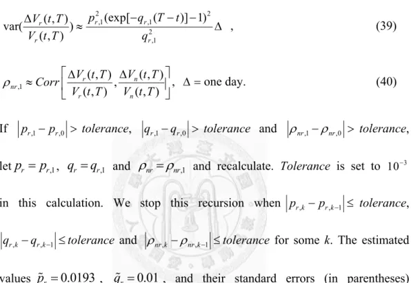
nr Corr  one day. (40) If p_r,1p_r,0  tolerance, q_r,1q_r,0  tolerance and _nr,1_nr,0  tolerance, letp_r  p_r,1, q_r q_r,1 and _nr _nr,1 and recalculate. Toleranc is see t to 10^3 in this calculation. We stop this recursion when p_{r k,} p_{r k, 1}  tolerance,

, , 1

r k r k

q q _  tolerance and _{nr k,} _{nr k, 1}  tolerance fo estimated .0193 , q_r 0.

and _nr

r k. The

, and their standard errors (in parentheses) some

values p_r  0.

0 126

01

  ^{able 2.}

Fig. 7 is the time-series graph of sprea are reported in T

ds during the of Jan

a

e period uary 17, 2000-October 23, 2009 (line). The estimated maximum value of spread is 2.16%,

nd the minimum value is -5%. The minimum spread occurred around Jan. 2009 while the CPI-U decreased drastically. Fig. 7 shows that an over-estimated spread between nominal and real rates is induced by ignoring the embedded option in TIPS during the period of January 17, 2000-October 23, 2009 (dashed line). Th

. (v) T

n embedded in each TIPS is shown in Fig. 8. TIPS7 is average difference between the distorted estimate and actual value is about 0.82%

he embedded option prices The estimated price of optio

the most expensive one since it is a long maturity bond with a larger CPI-U of issue date, while TIPS12 is the cheapest one since it is the shortest maturity bond with a smaller CPI-U of issue date. The CPI-U of issue date of TIPS7 is 211.08 while the CPI-U of issue date of TIPS12 is 190.9. The average prices of options embedded in TIPS of various maturity periods are shown in Table 3. The shorter is the maturity period, the cheaper is the embedded option price. Since the 30-year TIPS were issued much earlier than 20-year ones, the average CPI-U of the issue date of 30-year TIPS is smaller than that of 20-year ones. The average CPI-U of the issue date of 30-year TIPS is 168.8, while the average CPI-U of the issue date of 20-year TIPS is 202.5. It is apparent that the index ratios in 20-year TIPS are more likely to be smaller than 1. Therefore, the prices of options embedded in 20-year TIPS are more expensive than those embedded in 30-year ones. The embedded option consists of a portion of the TIPS value. The value of option embedded in the 20-year TIPS is about 18% of the TIPS value, while those embedded in the 30-year, 10-year and 5-year TIPS are about 12%, 6% and 3% of TIPS value, respectively. The percentages of options embedded in TIPS of various

1.6

form solutions for TIPS with stochastic volatility. At redemption, an maturity periods are shown in Table 3. The shorter is the maturity period, the smaller is the percentage. The percentage of option embedded in the 30-year TIPS is smaller than that embedded in the 20-year TIPS since the index ratios in 20-year TIPS are more likely to be smaller than 1.

Conclusion

We derived closed-

embedded option existed. Nominal rates and stochastic volatility were introduced into the determination of the valuation of TIPS through embedded options. The relationship between the embedded option price and the maturity, depending on nominal and real term structures and the reference CPI-U on the issue date is not monotonously ascending. The embedded option may comprise a portion of the TIPS value, reaching nearly 19%. An embedded option mispricing can result in a seriously distorted estimation of the nominal-TIPS spread which is often treated as future inflation rates.

Empirically, our model with 29 TIPS and treasury constant maturity rates was used to derive the unknown parameters and daily spread between nominal and real yields during January 2000 to October 2009. Empirical results show that an over-estimated spread between nominal and real rates is induced by ignoring the embedded option in TIPS.

The average difference between the distorted estimate and actual value is about 0.82%.

The value of option embedded in the 20-year TIPS is about 18% of the TIPS value,

osition I

while those embedded in the 30-year, 10-year and 5-year TIPS are about 12%, 6% and 3% of TIPS value, respectively. The shorter is the maturity period, the smaller is the percentage. Since the index ratios in 20-year TIPS are more likely to be smaller than 1, the percentage of option embedded in the 30-year TIPS is smaller than that embedded in the 20-year TIPS.

1.7 Appendices

Appendix A

Proof of Prop

, ( ) ,

(t T V t T

Z_n  _n ) B_n(0,t). Then, we have Define

dt du u t du

u t t

du u

dZ ^T

t n

 n^{( )}



)  

t T

t Z T

t ^T

t n

T

t n

n

n 



 



 





 



 ^{( , )}





) ,

(  

. (A1) From (A1), is -martingale iff

) *

, ( )

,

( ^T _n

t n

n t T t u du dW

Z 







) , ( Tt

Z_n Q







T

t n

T

t n t u du (t,u)du (t) (t,u)du

2 ) 1 ,

(  ²  

 (A2)

. (A3) Define _{r r} Then, we have



 



n^(t,T) n^(t,T)



, 0 ( ) ( )

(t I t B t

I 





t I t

dI_r( ) _r( )_I( )_In_n( )_Ir( )_r( ) ( )_I( ) _r( ) ) ( ) ( ) ( ) ( )

( ) ( )

(t dW^* t I t dW^* t I t Y t dW^* t

I_{r In n}  _{r Ir r}  _{r I}

   . (A4)

Define Z_Ir(t)I(t)B_r(0,t) B_n(0,t)I_r(t) B_n(0,t). Then, we have





t Z t

dZ_{I I I In n Ir r I r n}

r

r( ) ( ) ( )  ( ) ( ) ( ) ( ) () ( ) ( )