讀取大型資料

(1)

http://www.hmwu.idv.tw

吳漢銘國立政治大學統計學系

讀取大型資料

in R

D01

(2)

大綱



記憶體設置、物件大小、計算執行(資料讀取)時間



Handling Large Data Sets in R



讀取目錄下符合目標的(多個)檔案資料: list.files



直接讀取壓縮檔(zip)內之檔案



讀取HTML網頁表格，讀取XML表格



讀取影像檔案



從資料庫(MySQL)讀取資料



GREA: read ALL the data into R/Importing Data with RStudio



讀取部份資料進入R計算(readbulk)



fread {data.table}: Fast and friendly file finagler



讀取檔案部份欄位資料



如何讓read.table讀較大的資料速度更快

2/43

http://www.hmwu.idv.tw/index.php/r-software

(3)

> report.memory <- function(size = 4095){

+ cat("current memory in use: ", memory.size(max = FALSE), "Mb \n")

+ cat("maximum memory obtained from the OS: ", memory.size(max = TRUE), "Mb \n") + cat("current memory limit: ", memory.size(max = NA), "Mb \n")

+ cat("current memory limit: ", memory.limit(size = NA), "Mb \n") + cat("increase memory limit: ", memory.limit(size = size), "Mb \n") + }

>

> report.memory()

current memory in use: 686.74 Mb

maximum memory obtained from the OS: 1558.81 Mb current memory limit: 65408.91 Mb

current memory limit: 65408 Mb increase memory limit: 65408 Mb Warning message:

In memory.limit(size = size) : 無法減少記憶體限制：已忽略

Memory Allocation in R

^3/43

R與Windows作業系統

最大可穫得的記憶體

 32-bit R + 32-bit Windows: 2GB.

 32-bit R + 64-bit Windows: 4GB.

 64-bit R + 64-bit Windows: 8TB.



當R啟動時，設定最大可穫得的記憶體:

"C:\Program Files\R\R-3.2.2\bin\x64\Rgui.exe" --max-mem-size=2040M



最小需求是32MB.



R啟動後僅可設定更高值，不能再用

memory.limit

設定較低的值。

(4)

Report the Space Allocated for an Object:

object.size{utils}

 儲存R物件所佔用的記憶體估計。

object.size(x)

print(object.size(x), units = "Mb")

4/43

> n <- 10000

> p <- 200

> myData <- as.data.frame(matrix(rnorm(n*p), ncol = p, nrow=n))

> print(object.size(myData), units = "Mb") 15.3 Mb

> write.table(myData, "myData.txt") ## 約 34.7 MB

> InData <- read.table("myData.txt")

> print(object.size(InData), units = "Mb") 15.6 Mb

NOTE: Under any circumstances, you cannot have more than

2

³¹

-1=2,147,483,647 rows or columns.

(5)

object.size{utils}

^5/43

1 Bit = Binary Digit; 8 Bits = 1 Byte; 1024 Bytes = 1 Kilobyte; 1024 Kilobytes = 1 Megabyte 1024 Megabytes = 1 Gigabyte; 1024 Gigabytes = 1 Terabyte; 1024 Terabytes = 1 Petabyte

千萬佰萬

(n*p*8)/(1024*1024) MB

(6)

Measuring execution time: system.time{base}

^6/43

> start.time <- Sys.time()

> ans <- myFun(10000)

> end.time <- Sys.time()

> end.time -start.time

Time difference of 0.0940001 secs

> system.time({

+ ans <- myFun(10000) + })

user system elapsed 0.04 0.00 0.05 myFun <- function(n){

for(i in 1:n){

x <- x + i }

x }

See also : microbenchmark, rbenchmark packages

myPlus <- function(n){

x <- 0

for(i in 1:n){

x <- x + sum(rnorm(i)) }

x }

myProduct <- function(n){

x <- 1

for(i in 1:n){

x <- x * sum(rt(i, 2)) }

x }

> system.time({

+ a <- myPlus(5000) + })

user system elapsed 3.87 0.00 3.91

> system.time({

+ b <- myProduct(5000) + })

(7)

Handling Large Data Sets in R

 The Problem with large data sets in R:



R reads entire data set into RAM all at once.



R Objects live in memory entirely.



Does not have int64 datatype.



Not possible to index objects with huge numbers of rows &

columns even in 64 bit systems (2 Billion vector index limit) .

 How big is a large data set:



Medium sized files that can be loaded in R ( within memory limit but processing is cumbersome (typically in the 1~2 GB range ).



Large files that cannot be loaded in R due to R/OS limitations.

 Large files (typically 2 ~ 10 GB) that can still be processed locally using some work around solutions.

 Very Large files ( > 10 GB) that needs distributed large scale computing.

7/43

Handling large data sets in R, Sundar Pradeep & Philip Moy, April 10, 2015

https://rstudio-pubs-static.s3.amazonaws.com/72295_692737b667614d369bd87cb0f51c9a4b.html

https://msdn.microsoft.com/zh-tw/library/s3f49ktz.aspx

(8)

Strategy for Medium sized datasets (< 2 GB)



Reduce the size of the file before loading it into R (select some columns).



Pre-allocate number of rows (

nrows

) and pre-define column classes (

colClasses

), define

comment.char

parameter



Use

fread {data.table}

.



Use pipe operators to overwrite files with intermediate results and minimize data set duplication through process steps.



Parallel Processing



Explicit Parallelism (user controlled):

rmpi

(Message Processing Interface),

snow

(Simple Network of Workstations)



Implicit parallelism (system abstraction):

doMC

(Foreach Parallel Adaptor for 'parallel'),

foreach

(Provides Foreach Looping

Construct for R).

8/43

(9)

Strategy for Medium sized datasets (2 ~10 GB) and Very Large datasets (> 10GB)

 Medium sized datasets (2 ~ 10 GB)

 For medium sized data sets which are too-big for in-memory processing but too- small-for-distributed-computing files, following R Packages come in handy.

 bigmemory: Manage Massive Matrices with Shared Memory and Memory- Mapped Files (http://www.bigmemory.org/)

 ff: memory-efficient storage of large data on disk and fast access functions (http://ff.r-forge.r-project.org/)

 Very Large datasets (> 10GB)

 Use integrated environment packages like RHipe to leverage Hadoop MapReduce framework.

 Use RHadoop directly on hadoop distributed system.

(https://github.com/RevolutionAnalytics/RHadoop/wiki)

 Storing large files in databases and connecting through DBI/ODBCcalls from R is also an option worth considering.

9/43

(10)

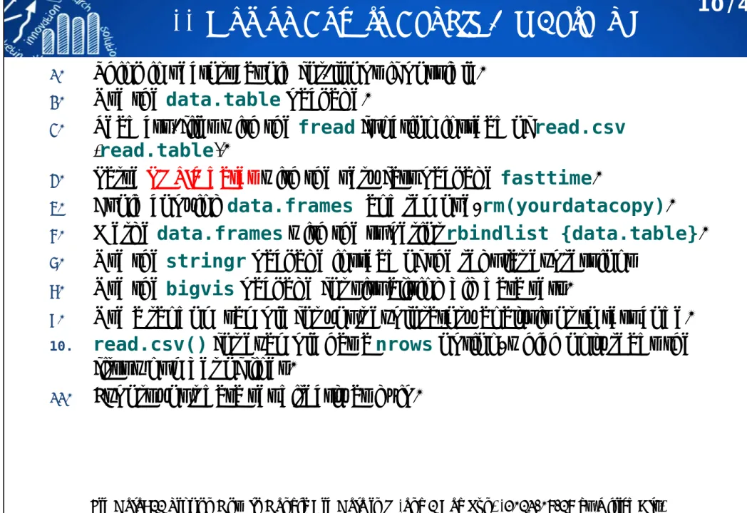
11 Tips on How to Handle Big Data in R

1.

Think in vectors: avoid for-loops if possible.

2.

Use the

data.table

package.

3.

Read csv-files with the

fread

function instead of

read.csv

(

read.table

).

4.

Parse POSIX dates with the very fast package

fasttime

.

5.

Avoid copying

data.frames

and remove,

rm(yourdatacopy)

.

6.

Merge

data.frames

with the superior

rbindlist {data.table}

.

7.

Use the

stringr

package instead of the regular expressions

8.

Use the

bigvis

package for visualising big data sets.

9.

Use a random sample for your exploratory analysis or to test code.

10. read.csv()

for example has a

nrows

option, which only reads the first x number of lines.

11.

Export your data set directly as gzip.

10/43

Fig Data: 11 Tips on How to Handle Big Data in R (and 1 Bad Pun) (2013-07-18 by Ulrich Atz) https://theodi.org/blog/fig-data-11-tips-how-handle-big-data-r-and-1-bad-pun

(11)

讀取目錄下符合目標的資料檔案: list.files

^11/43

> getwd() # setwd("F:/my_R") [1] "D:/R/data/quiz"

> list.files() # dir()

[1] "score_quiz1.txt" "score_quiz2.txt" "score_quiz3.txt" "score_quiz4.txt"

[5] "score_quiz5.txt"

> list.dirs() [1] "."

> (filenames <- list.files(".", pattern="*.txt"))

[1] "score_quiz1.txt" "score_quiz2.txt" "score_quiz3.txt" "score_quiz4.txt"

"score_quiz5.txt"

list.files(path = ".", pattern = NULL, all.files = FALSE, full.names = FALSE, recursive = FALSE,

ignore.case = FALSE, include.dirs = FALSE, no.. = FALSE)

10位學生(student.1~student.10)自由參加5次小考，各次小考之5科成績("Calculus" "LinearAlgebra"

"BasicMath" "Rprogramming" "English")分別紀錄於5 個檔案中。

(12)

讀取多個資料檔案並計算摘要

^12/43

> (quiz.data <- lapply(filenames, read.table)) [[1]]

gender Calculus LinearAlgebra BasicMath Rprogramming English student.5 M 69 93 83 79 95 student.4 M 70 78 31 26 69 ...

[[5]]

gender Calculus LinearAlgebra BasicMath Rprogramming English student.3 M 53 100 100 33 1 student.8 M 81 69 75 86 27 ...

> (quiz.data.summary <- lapply(quiz.data, summary)) [[1]]

gender Calculus LinearAlgebra BasicMath Rprogramming English F:5 Min. :56.00 Min. : 4.00 Min. : 8 Min. :15.00 Min. : 4.00 M:4 1st Qu.:62.00 1st Qu.: 6.00 1st Qu.:23 1st Qu.:26.00 1st Qu.:37.00 Median :69.00 Median :32.00 Median :43 Median :76.00 Median :62.00 Mean :67.11 Mean :44.89 Mean :45 Mean :63.33 Mean :57.11 3rd Qu.:73.00 3rd Qu.:78.00 3rd Qu.:73 3rd Qu.:95.00 3rd Qu.:69.00 Max. :76.00 Max. :97.00 Max. :83 Max. :99.00 Max. :97.00 ...

[[5]]

gender Calculus LinearAlgebra BasicMath Rprogramming English F:3 Min. :53.0 Min. : 14 Min. : 2.0 Min. : 9.0 Min. : 1 M:2 1st Qu.:53.0 1st Qu.: 15 1st Qu.: 39.0 1st Qu.:12.0 1st Qu.: 6 Median :70.0 Median : 32 Median : 55.0 Median :33.0 Median :27 Mean :66.2 Mean : 46 Mean : 54.2 Mean :43.8 Mean :31 3rd Qu.:74.0 3rd Qu.: 69 3rd Qu.: 75.0 3rd Qu.:79.0 3rd Qu.:41 Max. :81.0 Max. :100 Max. :100.0 Max. :86.0 Max. :80

> names(quiz.data.summary) <- filenames

> quiz.data.summary$score_quiz2.txt

(13)

課堂練習



合併此5組資料使成一資料表格，並新增一變數「小考次別(quiz.id)」



10位學生各參加哪幾次的小考?



各次小考，每科平均及變異數為多少? (未參加的同學不列入計算)



若此學期5次小考配分比重為(0.1, 0.1, 0.2, 0.2, 0.3)，

試計算每位同學各科小考平均及變異數?



每位同學每科皆刪除最差的一次成績，試計算每位同學各科小考平均及變異數?



男女生各科小考平均及變異數為多少?



試讀取單數次小考成績檔案進入R。

13/43

(14)

範例: 房屋實價登錄資料

^14/43

2014年臺灣資料分析競賽資料 (使用R軟體):

大約 682724筆紀錄，28個變數

(15)

範例: 房屋實價登錄資料

^15/43

(16)

Air Pollution Dataset from EPA

 Dataset: an air pollution (hourly

ozone levels) dataset from the U.S.

Environmental Protection Agency (EPA) for the year 2014.

http://aqsdr1.epa.gov/aqsweb/aqstmp/airdata/download_files.ht ml



U.S. EPA on hourly ozone

measurements in the entire U.S. for the year 2014. The data are available from the EPA’s Air Quality System web page.



The dataset is a comma-separated value (CSV) file, where each row of the file contains one hourly

measurement of ozone at some location in the country.

16/43

(17)

Hourly Data

^17/43

# dataset:

hourly_44201_2014.zip (64.7M) hourly_44201_2014.csv (1.89G)

(limited to 1,048,576 rows)

(18)

Hourly Data

^18/43

There are 34 variables with 8967571 observations:

"State Code","County Code","Site Num","Parameter Code", "POC",

"Latitude","Longitude","Datum","Parameter Name","Date Local",

"Time Local","Date GMT","Time GMT","Sample Measurement","Units of Measure",

"MDL","Uncertainty","Qualifier","Method Type","Method Code",

"Method Name","State Name","County Name","Date of Last Change"

註: 如何呈現這些變數的內容及資訊?

(19)

直接讀取壓縮檔(zip)內之檔案

^19/43

> library(readr)

> ozone <- read_csv("hourly_44201_2014.csv") # unzip and read

=================================================== | 96% 1900 MB

>

> # read without unzip

> # unz reads (only) single files within zip files, in binary mode.

> # The description is the full path to the zip file.

> # a zip file contains several files, create a connection to read one of the files

> # AirPollution-test.zip: hourly_44201_2014-test.csv, hourly_44201_2015-test.csv, hourly_44201_2016-test.csv

>

> zz <- unz(description="AirPollution-test.zip", filename="hourly_44201_2014-test.csv")

> ozone.zip <- read.csv(zz, header=T)

> ozone.zip

State.Code County.Code Site.Num Parameter.Code POC Latitude Longitude Datum Parameter.Name 1 1 3 10 44201 1 30.49748 -87.88026 NAD83 Ozone 2 1 3 10 44201 1 30.49748 -87.88026 NAD83 Ozone ...

> close(zz)

>

> # read from the web url

> location <- "http://aqsdr1.epa.gov/aqsweb/aqstmp/airdata/hourly_44201_2014.zip"

> zz <- unz(location, filename="hourly_44201_2014.csv")

> ozone.url <- read.csv(zz, header=T)

> close(zz)

See also: connections {base}: file(), url(), gzfile(), bzfile(), xzfile(), unz(), pipe() zz <- gzfile('file.csv.gz', 'rt')

mydata <- read.csv(zz, header=F)

(20)

讀取HTML網頁表格 (1)

^20/43

https://rstudio-pubs-static.s3.amazonaws.com/1776_dbaebbdbde8d46e693e5cb60c768ba92.html

https://www.drugs.com/top200_2003.html

> install.packages("XML", dep = T, repos="http://cran.csie.ntu.edu.tw")

> library(XML)

> library(RCurl)

readHTMLTable(doc, header = NA, colClasses = NULL, skip.rows = integer(), trim = TRUE, elFun = xmlValue, as.data.frame = TRUE,

which = integer(), ...)

(21)

讀取HTML網頁表格 (1)

^21/43

> URL1 <- getURL("https://www.drugs.com/top200_2003.html")

> htmlTable1 <- readHTMLTable(URL1, header=T)

> str(htmlTable1)

> head(htmlTable1[[1]])

(22)

讀取HTML網頁表格 (2)

^22/43

https://en.wikipedia.org/wiki/List_of_countries_and_dependencies_by_population

(23)

讀取HTML網頁表格 (2)

^23/43

> URL1 <- getURL("https://en.wikipedia.org/wiki/List_of_countries_and_

dependencies_by_population")

> htmlTable1 <- readHTMLTable(URL1, header = TRUE)

> str(htmlTable1)

> head(htmlTable1[[2]])

(24)

課堂練習

^24/43

http://www.boxofficemojo.com/alltime/world/

下載全球最高電影票房前500大電影紀錄:

• 票房分佈為何?

• 各發行商(Studio)之發行之電影數量為何?

• 各發行商(Studio)之平均每部電影之票房如何?

• 各年代之電影發行數量為何?

(25)

讀取 XML 檔案

^25/43

https://zh.wikipedia.org/wiki/XML

(26)

讀取 XML 檔案

^26/43

> library(XML)

> book.data <- xmlToDataFrame("books.xml")

> str(book.data)

> head(book.data)

https://msdn.microsoft.com/en-us/library/ms762271(v=vs.85).aspx

(27)

讀取影像檔案

^27/43

https://en.wikipedia.org/wiki/Transformers_(film)

> install.packages(c("tiff", "jpeg", "png", "fftwtools"), repos="http://cran.csie.ntu.edu.tw")

> library(EBImage) # (Repositories: BioC Software)

> Transformers <- readImage("Transformers07.jpg")

> (dims <- dim(Transformers)) [1] 300 421 3

> Transformers Image

colorMode : Color storage.mode : double dim : 300 421 3 frames.total : 3

frames.render: 1

imageData(object)[1:5,1:6,1]

[,1] [,2] [,3] [,4] [,5] [,6]

[1,] 0 0 0 0 0 0 [2,] 0 0 0 0 0 0 [3,] 0 0 0 0 0 0 [4,] 0 0 0 0 0 0 [5,] 0 0 0 0 0 0

> plot(c(0, dims[1]), c(0, dims[2]), type='n', + xlab="", ylab="")

> rasterImage(Transformers, 0, 0, dims[1], dims[2])

(28)

彩色影像轉成灰階

^28/43

> Transformers.f <- Image(flip(Transformers))

> # convert RGB to grayscale

> rgb.weight <- c(0.2989, 0.587, 0.114)

> Transformers.gray <- rgb.weight[1] * imageData(Transformers.f)[,,1] + + rgb.weight[2] * imageData(Transformers.f)[,,2] + + rgb.weight[3] * imageData(Transformers.f)[,,3]

> dim(Transformers.gray) [1] 300 421

> Transformers.gray[1:5, 1:5]

[,1] [,2] [,3] [,4] [,5]

[1,] 0 0 0 0 0 [2,] 0 0 0 0 0 [3,] 0 0 0 0 0 [4,] 0 0 0 0 0 [5,] 0 0 0 0 0

> par(mfrow=c(1,2), mai=c(0.1, 0.1, 0.1, 0.1))

> image(Transformers.gray, col = grey(

+ seq(0, 1, length = 256)), xaxt="n", yaxt="n")

> image(Transformers.gray, col = rainbow(256), + xaxt="n", yaxt="n")

Converting RGB to grayscale/intensity

http://stackoverflow.com/questions/687261/converting-rgb-to-grayscale-intensity

(29)

影像資料分析範例: Image Segmentation

 Segmentation: partition an image into homogeneous regions.

 Images: texture images, medical images, color images,...

 Medical Image Segmentation:

 anatomicalregions or pathologicalregions.

 extract tumors.

29/43

80 120 100

sd=20

FCM+FSIR

MRI images FCM+FSIR

Simulated images

(30)

Image Feature Extraction: Local Blocks

^30/43

grey level: f(x,y)=0,...,255

(31)

Image Features

^31/43

X

_64×9

Space Domain

Transformation

FFT Gabor Wavelet,..

. PCA SIR,...

Z

_64×p Segmentation Clustering Algorithms

Validation Indices

y₆₄

Cluster Label

(32)

讀取MySQL資料

^32/43

• 讀取Excel資料檔案

• 使用ODBC讀取 Excel 檔案 (Windows為例)

• 利用RMySQL

讀取MySQL資料庫的資料 (localhost)

• 利用RMySQL

讀取MySQL資料庫的資料 (remote host)

做適當設定

指定連線IP

MySQL

dbname = "bigdata105", username="student",

password="xxxxxx", host="163.13.113.xxx",

port=3306

(33)

課堂練習

^33/43

利用RMySQL (SQL語法) ，在表格

student.info填入個人資料(中英文皆可)。

SQL語法教學

http://www.1keydata.com/tw/sql/sql.html

(34)

GREA : read ALL the data into R



GREA: The RStudio Add-In to read ALL the data into R!

https://www.r-bloggers.com/grea-the-rstudio-add-in-to-read-all-the-data-into-r/



在RStudio安裝

> devtools::install_github("Stan125/GREA", force = TRUE)

> install.packages(c("csvy", "miniUI", "openxlsx", "readODS", "urltools"))

34/43

(35)

Importing Data with RStudio



Importing data into R is a necessary step that, at times, can become time intensive. To ease this task, RStudio includes new features to import data from: csv, xls, xlsx, sav, dta, por, sas and stata files.

35/43

https://support.rstudio.com/hc/en-us/articles/218611977-Importing-Data-with-RStudio

https://rstudio-pubs-static.s3.amazonaws.com/1776_dbaebbdbde8d46e693e5cb60c768ba92.html

(36)

readbulk : Read and Combine Multiple Data Files

^36/43

read_bulk(directory = ".", subdirectories = FALSE, extension = NULL, data = NULL, verbose = TRUE, fun = utils::read.csv, ...)

> raw.data <- read_bulk(directory = ".", extension = ".txt", sep=" ") Reading score_quiz1.txt

Reading score_quiz2.txt Reading score_quiz3.txt Reading score_quiz4.txt Reading score_quiz5.txt

> str(raw.data)

'data.frame': 39 obs. of 7 variables:

$ gender : Factor w/ 2 levels "F","M": 2 2 1 1 1 2 1 1 2 1 ...

$ Calculus : int 69 70 57 73 56 62 76 68 73 74 ...

$ LinearAlgebra: int 93 78 26 32 6 4 5 63 97 25 ...

$ BasicMath : int 83 31 21 73 50 73 8 43 23 0 ...

$ Rprogramming : int 79 26 99 76 98 22 95 15 60 28 ...

$ English : int 95 69 51 37 33 4 62 97 66 9 ...

$ File : chr "score_quiz1.txt" "score_quiz1.txt" "score_quiz1.txt"

"score_quiz1.txt" ...

> raw.data

gender Calculus LinearAlgebra BasicMath Rprogramming English File 1 M 69 93 83 79 95 score_quiz1.txt 2 M 70 78 31 26 69 score_quiz1.txt ...

38 F 70 32 55 79 6 score_quiz5.txt 39 F 53 15 2 9 80 score_quiz5.txt

(37)

fread {data.table} : Fast and friendly file finagler

37/43

library(data.table)

mydata <- fread("mylargefile.txt")

http://brooksandrew.github.io/simpleblog/articles/advanced-data-table/

https://cran.r-project.org/web/packages/data.table/index.html https://github.com/Rdatatable/data.table/wiki

https://www.datacamp.com/courses/data-table-data-manipulation-r-tutorial

Amazon EC2 r3.8large (Ubuntu, CPU(s): 32, Mem: 240G) fread(input, sep="auto", sep2="auto", nrows=-1L, header="auto", na.strings="NA", file,

stringsAsFactors=FALSE, verbose=getOption("datatable.verbose"), autostart=1L, skip=0L, select=NULL, drop=NULL, colClasses=NULL,

integer64=getOption("datatable.integer64"), # default: "integer64"

dec=if (sep!=".") "." else ",", col.names,

check.names=FALSE, encoding="unknown", quote="\"",

strip.white=TRUE, fill=FALSE, blank.lines.skip=FALSE, key=NULL, showProgress=getOption("datatable.showProgress"), # default: TRUE data.table=getOption("datatable.fread.datatable") # default: TRUE )

(38)

Demo Speedup

^38/43

https://www.rdocumentation.org/packages/data.table/versions/1.10.4/topics/fread

> n <- 1e6

> dt <- data.table(x1 = sample(1:1000, n, replace = TRUE), + x2 = sample(1:1000, n, replace = TRUE), + x3 = rnorm(n),

+ x4 = sample(c("foo", "bar", "baz", "qux", "quux"), n, replace = TRUE), + x5 = rnorm(n),

+ x6 = sample(1:1000, n, replace = TRUE) + )

> write.table(dt, "Speedup-test.csv", sep = ",", row.names = FALSE, quote = FALSE)

> cat("File size (MB):", round(file.info("Speedup-test.csv")$size / 1024 ^ 2), "\n") File size (MB): 51

>

> # read by read.csv

> system.time(data.rc <- read.csv("Speedup-test.csv", stringsAsFactors = FALSE)) user system elapsed

6.86 0.13 7.00

>

> # read by read.table, (all known tricks and known nrows)

> system.time(data.rt <- read.table("Speedup-test.csv", header = TRUE, + sep = ",", quote = "",

+ stringsAsFactors = FALSE, + comment.char = "",

+ nrows = n, colClasses = c("integer", "integer", "numeric", + "character", "numeric", "integer") + )

+ )

> # read by fread{data.table}

> system.time(data.fr <- fread("Speedup-test.csv")) user system elapsed

1.65 0.00 1.66

(39)

讀取部份資料進入R計算

^39/43

> cat(round(file.info('HIGGS.csv')$size /2^30, 2), "GB\n") 7.48 GB

>

> transactFile <- 'HIGGS.csv'

> readLines(transactFile, n=2)

[1] "1.000000000000000000e+00,8.692932128906250000e-01,-6.350818276405334473e- 01,2.256902605295181274e-01,3.274700641632080078e-01,-6.899932026863098145e-...

>

> variables <- c("label", "lepton_pT", "lepton_eta", "lepton_phi", "missing_energy_magnitude",

"missing_energy_phi", "jet_1_pt", "jet_1_eta", "jet_1_phi", "jet_1_b_tag", "jet_2_pt",

"jet_2_eta", "jet_2_phi", "jet_2_b_tag", "jet_3_pt", "jet_3_eta", "jet_3_phi", "jet_3_b-tag",

"jet_4_pt", "jet_4_eta", "jet_4_phi", "jet_4_b_tag", "m_jj", "m_jjj", "m_lv", "m_jlv",

"m_bb", "m_wbb", "m_wwbb")

http://archive.ics.uci.edu/ml/datasets/HIGGS

(40)

讀取部份資料進入R計算

^40/43

> chunkSize <- 100000

> con <- file(description=transactFile, open="r")

> dataChunk <- read.table(con, nrows=chunkSize, header=T, fill=TRUE, sep=",", + col.names=variables)

> index <- 0

> counter <- 0

> s <- 0

> repeat {

+ index <- index + 1

+ cat("Processing rows:", index * chunkSize, "\n") + s <- s + sum(dataChunk$lepton_pT)

+ counter <- counter + nrow(dataChunk) + if (nrow(dataChunk) != chunkSize){

+ print('Done!') + break

+ }

+ dataChunk <- read.table(con, nrows=chunkSize, skip=0, header=F, + fill = TRUE, sep=",", col.names=variables) +

+ if(index > 3) break # test this process in 3 times + }

Processing rows: 1e+05 Processing rows: 2e+05 Processing rows: 3e+05 Processing rows: 4e+05

> close(con)

> cat("number of observations: ", counter, "\n") number of observations: 4e+05

> cat("mean of lepton_pT: ", s/counter, "\n") mean of lepton_pT: 0.9923863

讀取檔案部份欄位資料

^41/43

> first.line <- readLines("HIGGS.csv", n=1)

> # Split the first line on the separator

> items <- strsplit(first.line, split=",", fixed=TRUE)[[1]]

> items

[1] "1.000000000000000000e+00" "8.692932128906250000e-01" "-6.350818276405334473e-01" "2.256902605295181274e-01"

[5] "3.274700641632080078e-01" "-6.899932026863098145e-01" "7.542022466659545898e-01" "-2.485731393098831177e-01"

[9] "-1.092063903808593750e+00" "0.000000000000000000e+00" "1.374992132186889648e+00" "-6.536741852760314941e-01"

[13] "9.303491115570068359e-01" "1.107436060905456543e+00" "1.138904333114624023e+00" "-1.578198313713073730e+00"

[17] "-1.046985387802124023e+00" "0.000000000000000000e+00" "6.579295396804809570e-01" "-1.045456994324922562e-02"

[21] "-4.576716944575309753e-02" "3.101961374282836914e+00" "1.353760004043579102e+00" "9.795631170272827148e-01"

[25] "9.780761599540710449e-01" "9.200048446655273438e-01" "7.216574549674987793e-01" "9.887509346008300781e-01"

[29] "8.766783475875854492e-01"

> length(items) [1] 29

> HIGGS.first2cols <- read.table("HIGGS.csv", header=F, fill=TRUE, sep=",",

+ colClasses = c(rep("numeric", 2), rep("NULL", 27)))

> str(HIGGS.first2cols)

'data.frame': 11000000 obs. of 3 variables:

$ V1 : num 1 1 1 0 1 0 1 1 1 1 ...

$ V2 : num 0.869 0.908 0.799 1.344 1.105 ...

> head(HIGGS.first2cols) V1 V2

1 1 0.8692932 2 1 0.9075421 3 1 0.7988347 4 0 1.3443848 5 1 1.1050090 6 0 1.5958393

colClasses: "character", "complex", "factor",

"integer", "numeric", "Date", "logical"

(42)

如何讓 read.table 讀較大的資料速度更快:

設定 colClasses



Specifying

colClasses

instead of using the default can make 'read.table' run MUCH faster, often twice as fast.



If all of the columns are "numeric", just set '

colClasses =

"numeric"

'.



If the columns are all different classes, or perhaps you just don't know, then you can read in just a few rows of the table and then create a vector of classes from just the few rows.

42/43

http://www.biostat.jhsph.edu/~rpeng/docs/R-large-tables.html

> system.time(data.rt1 <- read.table("Speedup-test.csv", header = TRUE, sep = ",")) user system elapsed

6.48 0.03 6.54

> system.time(tab5rows <- read.table("Speedup-test.csv", header = TRUE, sep = ",", nrows = 5)) user system elapsed

0 0 0

> classes <- sapply(tab5rows, class)

> classes

x1 x2 x3 x4 x5 x6

"integer" "integer" "numeric" "factor" "numeric" "integer"

> system.time(data.rt2 <- read.table("Speedup-test.csv", header = TRUE, sep = ",", + colClasses = classes))

(43)

如何讓 read.table 讀較大的資料速度更快:

設定 nrows, comment.char



Specifying the '

nrows

' argument doesn't necessary make things go faster but it can help a lot with memory usage.



If you know that the data rows are definitely less than, say, N rows, then you can specify '

nrows = N

' and things will still be okay. A mild

overestimate for '

nrows

' is better than none at all.

43/43

> # install.packages("R.utils")

> library(R.utils)

> system.time(n1 <- countLines("HIGGS.csv")) user system elapsed

32.44 22.50 55.00

> system.time(n2 <- length(readLines("HIGGS.csv"))) user system elapsed

308.24 7.36 315.78

> n1

[1] 11000000

attr(,"lastLineHasNewline") [1] TRUE

> n2

[1] 11000000

comment.char : If the data file has no comments in it (e.g. lines starting with '

#'

讀取大型資料

http://www.hmwu.idv.tw

吳漢銘 國立政治大學 統計學系