全並聯式線性驅動平台機構之局部運動特性分析
計畫類別: 個別型計畫
計畫編號: NSC92-2218-E-011-007-
執行期間: 92 年 08 月 01 日至 93 年 07 月 31 日 執行單位: 國立臺灣科技大學機械工程系
計畫主持人: 王勵群
計畫參與人員: 溫家俊
報告類型: 精簡報告
處理方式: 本計畫可公開查詢
中 華 民 國 93 年 10 月 28 日
行政院國家科學委員會專題研究計畫成果報告
全並聯式線性驅動平台機構之局部運動特性分析
Local Manipulability Analysis of Fully Parallel Linear Actuated Platform Type Manipulators
計畫編號:NSC 92-2218-E-011-007-
執行期限:92 年 8 月 1 日至 93 年 7 月 31 日 主持人:王勵群 國立台灣科技大學機械系
中文摘要
本計畫結合解析法及數值分析法,研發出一套有 效率且系統化的方法來分析 Stewart Platform 類 型之全並聯式線性驅動平台機構的三項局部運動 特性問題。第一項問題為分析此類機構於任意指 定位置時,其活動平台可沿裝置於其上之工具主 軸方向自由轉動的最大容許旋轉角度。第二項問 題為分析工具主軸相對於任意指定之活動平台位 置及方位的最大容許傾斜角度。第三項問題則為 探討活動平台於任意指定位置之三自由度方位工 作空間的建立方法。此三項問題皆受限於並聯式 機構之三類運動拘束條件,即各線性驅動器之運 動衝程限制,機構中之球接頭及萬向接頭等被動 接頭的旋轉角度限制,以及各連桿間之干涉條件 限制。
關鍵詞:並聯式機構,局部運動特性分析
Abstract
A unified hybrid analytical-numerical computational algorithm is developed in this project for solving three problems in associated with the local manipulability of the Stewart type fully parallel linearly actuated platform manipulators. The first problem is to find the physically allowable region that the moving platform can be freely rolled about any given direction of the spindle axis of the tool bit at any specified position. The second problem is to investigate the maximum allowable tilt angle of the spindle axis about any given position and orientation of the moving platform. The third problem is to generate the three dimensional orientation workspace of the moving platform with respect to the given position of the tool bit. The kinematic constraints involved in these problems are the actuator stroke limitations, the physical motion limitations of the passive spherical and universal joints, and the link interference considerations.
Keywords: Parallel Mechanism, Local Manipulability Analysis
1. Introduction
In recent years, many researchers have studied the workspace properties of parallel manipulators.
Yang and Lee1investigated the positioning workspace of a special case of the 6-SPS (Stewart) platform manipulator with restricted rotatability. Gosselin2 presented a geometrical properties based algorithm for finding the positioning workspace of the Stewart platform with a given orientation of the platform.
Masory and Wang3presented a numerical method for evaluating the reachable workspace of Stewart platforms under the constraints of link length, joint angle limitations, and link interference. Wang and Hsieh4 developed a unified computational algorithm based on nonlinear programming techniques for finding the reachable workspace of general parallel manipulators. Marlet5 has developed a method for synthesizing the dimensions of the manipulator according to workspace requirements which described by a set of geometric objects such as points and line segments. In addition to the positioning workspace, Yang and Haug6-7have proposed a numerical method for analyzing the dextrous workspace and dextrous orientation capability of mechanisms, where they have taken into account the loop closure constraints of the mechanism. On the other hand, Kim, Chung and Youm8 have presented a generic numerical approach for finding both the reachable and dexterous workspace of six degrees of freedom parallel robots subjected to position and mechanism constraints.
Most of the above researches investigate the workspace of parallel mechanisms from a global point of view. However, when using a six-degree-of- freedom platform type robot to perform five-axes machining process, the local manipulability of the mechanism is also an important property to be considered. Specifically, for three dimensional contour milling process, one needs only specifying the position and the direction of the tool bit along the given motion trajectory, and hence the rotation of the platform about the spindle axis of the tool bit becomes a redundant degree of freedom. From advanced trajectory planning point of view, this redundant degree of freedom is useful for adjusting the configuration of the manipulator along the trajectory to avoid possible singularities or to optimize the dynamic performance
studied. The first problem is to find the physically allowable region that the moving platform can be freely rolled about any given direction of the tool bit at any specified position. The second problem is to investigate the maximum allowable tilt angle of the tool bit about any given position and orientation of the moving platform. The third problem is to analysis the three dimensional orientation workspace of the moving platform with respect to the given position of the tool bit. The kinematic constraints involved in these problems are the limb length limitations, the physical motion limitations of the passive spherical and universal joints, and the link interference considerations. In order to solve these problems efficiently and also taking into account all of the constraints, a unified hybrid analytical-numerical computational algorithm is developed.
2. Definition of Local Manipulability Problems
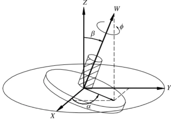
As shown in Figure 1, the W axis of the moving frame U-V-W attached to the moving platform is coincided with the spindle axis of the tool bit, and the origin of the frame is located at point C, which is also a point fixed on the spindle axis. The three local manipulability problems investigated in this paper are defined below.
PC W
X Y Z
O
U V C
Tool bit
Spindle axis
Figure 1. Definition of coordinate systems Rolling Capability
Given the absolute position of point C, PC, and a unit vector w along the positive W axis to denote the direction of the spindle axis, the rolling capability is defined as the allowable range of the angle that the moving platform can be rotated about w without violating the kinematic constraints of the robot.
Tilting Capability
As shown in Figure 2, for a given position and orientation of the moving platform, and let k be a
swinging k about the W axis for one revolution and simultaneously evaluating the tilting capabilities, the allowable tilting boundary of the moving platform for the given position can be plotted as a curved cone as shown in the figure. Consequently, the cone generated with respect to the minimum tilting capability, min, is defined as the usable tilting boundary9, as the moving platform can be tilted within this cone about any direction specified on the U-V plane.
min
Z
W
U
V
k Allowable tilting
boundary
Usable tilting boundary
Figure 2. Definition of the tilting boundaries Orientation Workspace
With the above definitions of the rolling and tilting capabilities, the orientation workspace of the robot at a given position is defined as the three-dimensional space that the moving platform can be rolled and tilted without violating any of the kinematic constraints. The boundary surface of the orientation workspace can be plotted against the three Euler angles , β, and
as shown in Figure 3, where is the angle measured from the positive direction of the fixed X axis to the projected vector of the W axis onto the X-Y plane, and βand are respectively the tilting angle and the rolling angle of the moving platform.
X
Y Z
W
Figure 4. Definition of the orientation workspace.
3. Formulation of the Kinematic Constraints
Limb Interference
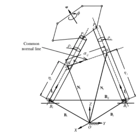
The coupled kinematic loops of the LAPs are formed by the limbs connecting the moving platform and the base. As shown in Figure 5, when the moving platform is commended to rotate about a given point C with respect to a specified axis of rotation w, the limbs may obstruct or collide to each other and hence restricts the allowable range of the rotation.
Pi
Pj
ρj
i
ij nij
Nj
Ni
i
Ni Nj
lj
li
Bij
Bj Bi
Bi Bj
j
Y Z
X Common
normal line w
O
Figure 5. Limbs interference condition Te shapes of the limbs are assumed to be cylindrical with radius of i (i = 1 to 6). The interference condition between any two limbs i and j, therefore, can be evaluated by monitoring the normal distance
ij between the two limbs vectors Liand Lj, as well as the location of the intersection points, Niand Nj, of the common normal line and the two lines defined by Liand Lj. If ij ij, then the following three cases should be examined in order to determine whether a physical interference between these two limbs is occurred or not.
Case 1.
i iL
or 0
i , and
j jL
or 0
j
In this case, the two limbs are not actually interfered to each other, as the intersection point is not within the physical length of the limbs.
Case 2. 0iLi and
j
j L
0
In this case, the intersection point is within the physical length of the limbs, and hence the interference is actually occurred.
Case 3.
i
i L
and j Lj (or
i iL
and
j jL
)
This is the case where Nj is outside of the physical length of limb j while Niis inside the physical length of limb i (or vice versa). This indicates that the interference between the two limbs may be occurred if
the top of the limb j should have contacted or penetrated into the outer surface of limb i as illustrated in Figure 6.
Pi
Pj 0
j
j
lj
Pj Cj 0
i
) (i
i
i
Si
i
li
Bi Bi
Y X
Z
O
Figure 6. Parametric representation of the outer surfaces of the limbs
By combining the parametric form of the cylinder surface equation of limb i and that of the top circular edge of limb j using theSylvester’sdialyticmethod10, one obtains
0
8
0
k
k i kt
A (1)
where Ak (k = 0 to 8) are constant coefficients and )
2 tan( i
ti . If there exists any real solutions to equation (1), then it can be concluded that the two limbs are indeed interfered to each other at the current configuration.
Actuator Stroke Constraints
The stroke constraints for the linear actuators can be written as
u i i l
i q q
q ,for i = 1 to 6 (2)
where qi denotes the joint variable of the ithdriving joint of the robot, qil and qiu are respectively the lower and the upper bound of the stroke of the linear actuator attached to the joint.
Passive Joints Constraints
The passive joints are the universal joint and the spherical joint that attached to the two end points of each limb. As in general the spherical joint would allow the limb to be freely rotated about its own axis, the constraints of both types of passive joints can be considered as the same. As illustrated in Figure 6, once a joint is physically installed on the base or the moving platform, the normal direction of the joint is known and can be denoted as a unit vector nj, and the upper bound of the limb that can be tilted about any
j
nj
u
j
Bi
Figure 7. Motion boundaries of the passive joints Therefore the general form of the passive joint constraint can be written as
u j j u
j
(3)
where j denotes the current tilting angle of the limb, and it is given by
) ( cos1 i j
j l n
(4)
4. Link Interference Analysis
In order to evaluate the allowable angles that the moving platform can be rotated about a specified direction without violating the limb interference constraint, it is necessary to first establish the functional relationship between the limb vectors Li(i = 1 to 6) and the rotation angle .
W
V U C
Z
Y
X O
() Pi
() Li
Li
PC
Pi 0
ri
Bi Bi
Figure 8. Vector loop closure relation of the Limb As shown in Figure 8, the vector loop equation for the ithlimb is given by
i i C
i P R w r B
L () ( ,) 0 (5)
spatial rotation matrix. Based on equation (5) and the definition of link interference presented in the previous section, the interference condition between any two links can be derived as
4 0
0
k k kt
B (6)
where Bk (k = 0 to 4) are constant coefficients and )
2 tan(
t . The above equation can have at most four real solutions of . This implies that when one rotates the moving platform about the given axis of rotation, there may exist four intersection points between the two limbs. It should, however, be noted that only two of these points may actually exist to obstruct the rotation, as illustrated in Figure 9, where angles 2 and 3 are physically unattainable in both clockwise and counterclockwise directions.
j
i
1
2
3
4
Figure 9. Possible limb intersection points
5. Analysis of the Stroke Constraints
The functional relationship between the joint variable of the actuators and the rotational angle of the moving platform can be established by squaring both sides of equation (5). After substituting the tangent half angle formulae for the rotation angle and rearranging terms, one obtain
2
0 2
k k k
i E t
l (7)
in which ttan(2), and Ek(k = 0 to 2) are constant coefficients. The stroke constraints of the linear actuators are given by equation (2). By substituting the bounds qil and qiu of the joint variables into equation (7), the stroke constraints can be expressed in the general form as
2 0
0 ) (
k
k l i
k q t
F (8)
and
2
0
0 ) (
k
k u i
k q t
F (9)
where Fk(qil) and Fk(qiu) (k = 0 to 2) are constant coefficients in terms of the upper and lower bounds of the ith actuator respectively. Noting that each of the above two equations can have at most two distinct real solutions, and hence the allowable rotation range of the moving platform with respect to the stroke limitation of each joint can be evaluated from the intersection region of these two solution sets.
6. Analysis of the Passive Joint Constraints
The passive joint constraint is given by equations (3) and (4), by introducing equation (5) into these equations, the functional relationship between the bounds of the tilting angle of the limbs and the rotation angle of the moving platform can be written in the general form as
j i u
j l ( )n
cos (10)
where li()Li() Li() . By substituting the tangent half angle formulae into equation (10) and rearranging terms, the passive joints constraints can be formulated into a polynomial equation as
0
4
0
k
k kt
G (11)
in which Gkare constant coefficients. Nevertheless, the above equation can have at most two distinct real roots of to satisfy equation (10) (the other roots are either complex conjugate pairs or superfluous roots and should be ignored), and which are corresponding to the extreme rotation angles of the moving platform against the constraint of the particular passive joint.
7. Computational Algorithms
Rolling Capability
Step 1. Specify the position vector PCand the desired direction w of the spindle axis of the tool bit.
Step 2. By using the methods described in section 4, compute the rotational range of the moving platform between the intersection points of each pair of adjacent limbs (i.e. limbs 1 and 2; 2 and 3; etc.) as
] [
Rintfi il iu . Hence the intersection region of these ranges, 61
intf
intf R
D
i i , is the region that the moving platform can be rotated without violating any of the interference constrains.
Step 3. By using the methods presented in section 5,
compute the rotational ranges of the moving platform limited by the stroke constraints of each actuator as
] [
Rstrki il iu , for i = 1 to 6. The allowable region for avoiding all of the stroke constraints thus is
61 strk
strk R
D
i i .
Step 4. Compute the rotational ranges of the moving platform due to each of the passive joint constraints by using the method presented in section 6 as
] [
Rjntj lj uj , for j = 1 to 12. Consequently, the overall rotational region of the moving platform due to the passive joint constraints is
121jnt
jnt R
D j j . Step 5. Compute the rolling capability as
strk jnt
intf D D
D
D .
Tilting Capability
Step 1. Input the position vector PCand the orientation matrix [R] of the moving platform. Specify a small increment angle and initialize 0.
Step 2. Compute the tilting direction
R cos sin 0t
k ,
and then using the rolling capability algorithm just described to determine the tilting capability of the moving platform with respect to PCand k asD(). Step 3. Set . If 2 , then go to step 2, otherwise compute the minimum tilting capability as
minmin D( ), 0 2 .
Orientation Workspace
Step 1. Input the position vector PC, specify the increment angles and , and initialize 0. Step 2. Compute the tilting direction
cos sin 0t
k ,
and then compute the upper and lower bound of the tilting capability with respect to PC and k as l and
u. Initialize .l
Step 3. Compute the rolling direction
]t
cos sin sin sin cos
[
w ,
and then compute the upper and lower bound of the rolling capacity with respect to PC and w as l and
u . Save the current valuesof(α,β,l)and (α,β,
u ) into two record sets.
Step 4. Set . If u, then go to step 3, otherwise go to the next step.
Step 5. Set . If , then go to step 2, otherwise go to the next step.
Step 6. Construct a three dimensional plot of the orientation workspace from the data of the record sets.
8. Numerical Example
The schematic diagram of the Stewart platform used for the example is shown in Figure 10, whereas the
X
Y Z
U V C
b3
b1
b6
b5
b4
PC
p1
p2
p3
p4 p5 p6
O b2
Figure 10. Schematic diagram of the Stewart platform
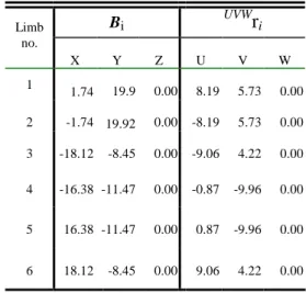
Table 1. Geometric dimensions of the Stewart LAP
Bi UVWri
Limb no.
X Y Z U V W
1 1.74 19.9 0.00 8.19 5.73 0.00
2 -1.74 19.92 0.00 -8.19 5.73 0.00 3 -18.12 -8.45 0.00 -9.06 4.22 0.00 4 -16.38 -11.47 0.00 -0.87 -9.96 0.00
5 16.38 -11.47 0.00 0.87 -9.96 0.00
6 18.12 -8.45 0.00 9.06 4.22 0.00
The stroke limitations of the limbs are designated to [qil qiu ] = [15.0cm 40.0cm] , for i = 1 to 6. The normal axis of the passive joints are installed along the directions of the limbs at the home position, the rotational bound of these joints and the radius of the limbs are respectively designated to uj 60, for j = 1 to 12, and 1.0
i cm, for i = 1 to 6. The position vector of the tool bit is given by PC0 0 25cmt. The initial orientation matrix of the moving platform at each individual configuration is computed from
C S S C S S S S S C
S S S S
S C S S S S C S S C
2 2 2
2
2 2
2 2 2 2
2
1 1
1 0
1 1
R
in which
C ,a C, S, and S denote the cosine
Figure 11. Orientation Workspace
9. Conclusions
An in-depth investigation of three local manipulability problems in associated with the Stewart platform type of fully parallel LAPs has been conducted, and a unified approach for solving these problems has been presented. This approach takes into account three types of kinematic constraints, namely the link interference condition, the passive joint limitation, and the actuator stroke constraint. It is shown that instead of using time consuming exhausted numerical search algorithms, all of these constraints can be handled analytically.
The knowledge of local manipulation properties is particularly useful for fine tuning the configuration of the robot to avoid singularities or to improve dynamic performance along specified motion trajectories.
Therefore, it is believed that the methods developed in this study can be further incorporated with optimization techniques to carry out such advanced off-line trajectory planning tasks for the LAPs.
References
[1] D.C.H. Yang and T.W. Lee, Feasibility study of a platform type of robotic manipulators from a kinematic viewpoint, ASME J. Mechanisms, Transmissions, and Automation in Design, 106 (1984), 191-198.
[2] C. Gosselin, Determination of the workspace of 6-dof parallel manipulator, ASME J Mech Des, 112 (1990), 331-336.
[3] O. Masory and J. Wang, Workspace evaluation of Stewart platforms, Advanced Robotics, 9:(4) (1995), 443-461.
[4] L.-C. T. Wang and J.H. Hsieh, Extreme reaches and reachable workspace analysis of general parallel robotic manipulators, J Robot Syst, 15:(3)
(1998), 145-159.
[5] J.-P. Merlet, Designing a parallel manipulator for a specific workspace, Int J Robot Res 16:(4) (1997), 545-556.
[6] F.C. Yang and E.J. Haug, Numerical analysis of the kinematic dexterity of mechanisms, ASME J Mechl Des, 116 (1994), 119-126.
[7] F.C. Yang and E.J. Haug, Numerical analysis of the kinematic working capability of mechanisms, ASME J. Mech Des 116(1994), 111-129.
[8] D.I. Kim, W.K. Chung and Y. Youm, Geometrical approach for the workspace of 6-dof parallel manipulators, Proc IEEE ICRA, 1997, pp.2986-2991.
[9] Z. Wang, W. Liu, and Y. Lei, A study on workspace, boundary workspace analysis and workpiece positioning for parallel machine tools, Mech Mach Theory, 36 (2001), 605-622.
[10] G. Salman, D.D., Lessons Introductory to the Modern Higher Algebra, fifth edition, Chelsea publishing company, Bronx, New York, pp.79-81.