三自由度機器人之工作空間以及最佳設計之研究

(1)

行政院國家科學委員會專題研究計畫成果報告

三自由度機器人之工作空間以及最佳設計之研究研究成果報告(精簡版)

計畫類別：個別型

計畫編號： NSC 97-2221-E-011-051-

執行期間： 97 年 08 月 01 日至 98 年 07 月 31 日執行單位：國立臺灣科技大學機械工程系

計畫主持人：蔡高岳

報告附件：出席國際會議研究心得報告及發表論文

處理方式：本計畫可公開查詢

中華民國 98 年 10 月 14 日

(2)

行政院國家科學委員會補助專題研究計畫成果報告

※※※※※※※※※※※※※※※※※※※※※※※※※※

※ ※

※※※※※※※※※※※※※※※※※※※※※※※※※※

計畫類別 : 個別型

計畫編號 : NSC 97-2221-E-011-051-

執行期間 : 97 年 08 月 01 日至 98 年 07 月 31 日執行單位 : 國立台灣科技大學機械工程系

計畫主持人 : 蔡高岳

計畫參與人員: 碩士班研究生-兼任助理人員 : 陳俊宏碩士班研究生-兼任助理人員 : 黃亭淵博士班研究生-兼任助理人員 : 李庭官

處理方式 : 本計畫可公開查詢

中華民國 98 年 10 月 13 日

研究成果報告(精簡版)

三自由度機器人之工作空間以及最佳設計之研究

(3)

行政院國家科學委員會專題研究計畫成果報告

三自由度機器人之工作空間以及最佳設計之研究

計畫編號 : NSC 97-2221-E-011-051-

執行期限 : 97 年 8 月 1 日至 98 年 7 月 31 日

主持人 : 蔡高岳國立台灣科技大學

共同主持人 :

計畫參與人員 : 李庭官、陳俊宏、黃亭淵

國立台灣科技大學中文摘要

操控性與工作空間為設計機器人時之兩個重要參考指標。此計劃利用三次多項式之解析解提出數個方法求得具有不同操控性指數之操控性曲面。由這些曲面之分布情形及其所包含區域之體積之大小可用來評估一機器人之整體操控性以及操控性之變化率，而軸位移空間之一曲面可用來求得工作空間內之一封閉邊界曲面並使曲面內任一點之操控性指數值均大於某一特定值

。所提出之方法可應用於設計具有最佳操控性或最大(操控性指數值均大於某一特定值之)無奇異點工作空間之三自由度機器人或四自由度多餘軸機器人。

關鍵詞:等向性，操控性，工作空間，奇異點，最佳設計，三自由度機器人

ABSTRACT

Dexterity and workspace are two of the most important design criteria in developing manipulators. This work employs the analytical solutions of the cubic to present algorithms for developing contour surfaces with specified dexterities. The obtained results can be utilized to evaluate the dexterity, rate of change of dexterity, or homogeneity in the distribution of the contour curves or surfaces. Any closed curve or surface can be employed to determine the singularity-free workspace of a manipulator with dexterity better than a specified value.

The proposed algorithms can be utilized to develop 3-DOF manipulators or 4-DOF

redundant serial manipulators with optimum dexterity or singularity-free workspace.

Keywords: isotropy, dexterity, workspace, singularity, optimal design, 3-DOF manipulator.

1. Introduction

Except for manipulators used in some special applications, dexterity is a very desirable property for almost any type of manipulators.

Dexterity can be evaluated by several measures [1] in which the condition number is the most commonly used mathematical tool to evaluate local dexterity of a manipulator. If the condition number (or the reciprocal of the condition number) of a related matrix reaches the optimum value of unity, then a manipulator is at an isotropic configuration where the manipulator can be controlled equally well in all directions, and sensitivity in velocity and force analysis is at a minimum. The dexterity of a manipulator, in general, is evaluated by

1

w

dW dW



  



 



^,

where  is the condition number at a particular point in workspace, and the denominator is the volume of the workspace [2-4]. It measures the average performance of a manipulator. This approach, however, cannot determine which region or which branch of kinematic solutions has better dexterity or evaluate the rate of change of dexterity. Thus, local dexterity still might change significantly even for manipulators with good dexterity. For lower

(4)

degree-of-freedom manipulators, some researcher [5, 6] have employed atlas of dexterity curves to develop manipulators with optimum dexterity. The dexterity and the rate of changes of dexterity can be seen from the distribution of the curves. However, it is difficult to see the related positions of dexterity surfaces for higher degree-of-freedom manipulators.

In this work, algorithms based on the analytical solutions of the cubic are employed to develop atlas of dexterity surfaces. Some related properties about dexterity (such as the global dexterity of a manipulator, the dexterity for a particular group of contour surfaces or a particular branch of kinematic solution, rate of change of dexterity, the area of a boundary surface or volume enclosed in the surface with desired dexterity, or the relative positions of two neighboring surfaces) can be estimated from the atlas and some related data obtained in the developing process. Any surface in joint space with specified dexterity can be utilized to develop the boundary of a region in workspace with dexterity better than the specified value. The algorithms can be employed to develop 3-DOF manipulators or 4-DOF redundant serial manipulators with optimum dexterity or singularity-free workspace. In theory, the methods can be extended to higher degree-of-freedom manipulators because the dexterity of a 6 DOF or redundant manipulator can also be evaluated by the solutions of the cubic [7].

2. Formulas and applications

This section provides formulas for the maximum solution and the minimum solution of the 3^rddegree characteristic equations of a positive semidefinite matrix and then employs them to evaluate the dexterity of a manipulator. The cubic can be arranged as

0 a x a 3 x a 3 x ) x (

f  ³ ₁ ²  ₂  ₃  (1) Let H =a₂a₁², G =a₃3a₁a₂2a₁³and,



² ³



1 4

p2  G i G  H . Then the maximum

solution and the minimum solution of the equation are [7]

13

max 2 cos 1

x  r    3 a (2)

13

min 1

2 sin 7

6 3

x  r ^  ^a (3)

where r and  denote the amplitude and argument, respectively, of p . In this work, the dexterity is evaluated by the reciprocal of the condition number, or

min max

x

 x

A point in joint space is on a curve or surface with a specified  if the joint displacements satisfy

1 2 min max

( , ,.., _n) 0

f q q q  x  x 

where q denotes_i the i^th actuated joint displacement. The equation and the bisection method will be employed to develop contour surfaces with specified dexterities.

At least one real solution of f(x) = 0 can be found in the closed set [a, b] by the bisection method if f(a) = 0, f(b) = 0, or f(a) f(b) 0. In the first application, the bisection method, the mod (modulus after division) function, and a grid-scanning technique are utilized to develop dexterity surfaces with k

  nfor k

= 1, 2, 3, .., n-1. The following two functions:

( )

g  n- mod(n, 1) (6) ( _A, _B) ( _A) ( _B)

h    g  g  (7)

will be employed to facilitate the searching process, where function h yields the number of desired points that can be obtained from the two starting points A and B. Note that mod(r, 1) yields the part after the decimal (4)

(5)

point of a real number r. Suppose that

B A

  , n = 20, and h = 2. Then two points P and1 P with₂

P1

 = ( ( ) 1) / 20g  _B and

P2

 = ( _B) / 20

g  can be obtained. For example, if

 = 0.21 andB  = 0.12, then_A

P1

 = 0.15 and

P2

 = 0.2 can be developed by the bisection method. First, points A and B are utilized to develop pointP with₁

P1

 _A. ThenP₂ is developed from P and B. The searching₁ process can be significantly improved if a larger step is chosen in the grid-scanning method, but some desired points might not be obtained when two points with  ≅_A B

are used in the bisection method. In this case, the obtained results may not be closed curves or surfaces.

The dexterity for a particular group of contour surfaces is easier to evaluate using spherical coordinates. With the point with local optimum  (denoted by ) as the_max origin, the joint displacements can be defined by

*

1 1

*

2 2

*

3 3

sin cos sin sin cos

q q

  

 

 

(8)

where 0   , 0  2 , and q^* 

* * *

1 2 3

(q q q, , )denotes the point with  . With_max parameters φ and θ given, the points with desired dexterities on the straight line through the origin with  as the free parameter can be developed without using a grid-scanning approach. If a point on the straight line with ¹

 n is obtained, then points on the line with ^{2 3}, ,...,k

n n n

 can

be developed using the bisection method with the origin and the point with ¹

n as two starting points, where k is the maximum integer satisfying k _max.

n Therefore, a particular group of contour surfaces with

different dexterities can be developed using a 2-dimensional grid-scanning method through parameters φ and θ.

The area of the i^th grid on the surface with a specified  can be approximated by Agi =

2

i i i

    , where  is the distance from_i the origin to the center of the grid. The area of the surface can be estimated by _gi

1

A

n



i

with n represents the number of grids. If each grid uses the same  and , then the area is proportional to ²

1

.

n i i





 ^Let ^^⁼^^^.

Then the volume of the region enclosed by the surface can be estimated by

3 2

i

1 1

1 ( ) 3

n n

i

i i

 

 

  

 

^, ^where ^{ is the}ⁱ

volume of a pyramid with the i^th grid as the base and the origin as the vertex. Therefore, the volume is proportional to ³

1

.

n i i





 ^{All the}

points in the region has dexterity better then the specified . Either ²

1 n

i i





 ^or ³ 1 n

i i





 ^can

be employed to evaluate which group of contour surfaces or which branch of kinematic solutions has better dexterity. For manipulators with joint limits, the  and_i²

3

 are excluded from the summations if anyi

joint displacement exceeds its limits.

LetV_j denote the volume of a region with j.

n Then the volume of a region with

1 2

j j

n   n equals to

1 2

j j

V V . In theory, the difference in volume can be used to estimate the average rate of change of dexterity for the points in the region. However, the relative positions of the two surfaces with  = j¹

n and  = j²

n , respectively, cannot be determined by this approach. The distance from a point P_i with  = j²

n to an

(6)

associated point Q_i with  = j¹

n can be used to detect the relative position of the two boundary surfaces. Point Qiis on the straight line defined by point Pi and the direction specified by the gradient (in 3D space) of  at Pi. The point, which is at the opposite direction of the gradient, can be easily obtained using the bisection method. The average length Lave of line segments of PiQi

can be employed to evaluate the average rate of change of dexterity for points between the two surfaces, and the ratio of the minimum length L_min to the maximum length L_max can be utilized to check the relative position of two neighboring surfaces. Better rate of change and distribution of dexterity surfaces can be expected for larger Lave and

min max

L

L .

More accurate results of the area of the boundary surface and the volume of the enclosed region can be computed using Cartesian coordinates. This approach takes consecutive cross-sections with one q_j-axis as the common normal. Let A denote the area_i of the 2D region on the i^th cross-section and s represent the length of its closed boundaryi

curve. Then the volume of the 3D region V_j

with j

 n and the area of the boundary surface _jwith j

 ncan be evaluated by V_୨= ∑^{୫ ିଵ}_୧ୀଵ ^ሺ୅^౟^ା୅_ଶ^౟శభ⁾∆q_୨ (9) Ω୨= ∑୫ ିଵ^ሺୱ^౟^ାୱ_ଶ^౟శభ⁾∆q୨

୧ୀଵ (10)

where m and Δq୨ denote the number of cross-section taken and the distance between two neighboring sections respectively.

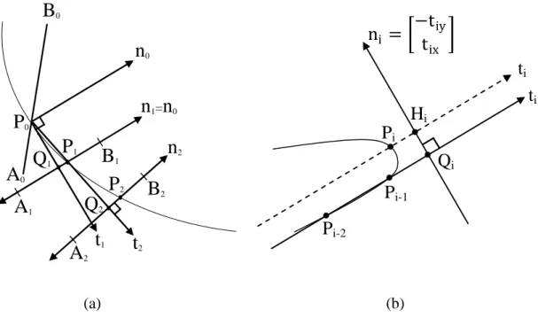
A closed curve on the i^thcross-section with specified dexterity of  =  can be_s developed using the bisection method. Figure 1a shows the steps to develop a contour curve with  =  . First, the starting point_s Po can be obtained by finding two points Ao

and Bo such that condition

Ao

 < <_s

Bo

 is satisfied. To avoid getting two points from different group of contour curves, the

gradient (approximated by

1 2

[ , ]^t

q q

 

 

  ) at the first point Ao can be utilized to find the second point. Search for point Boin the direction of the gradient if

Ao

 <  . Otherwise, search for the point in_s the opposite direction of the gradient. Next, the gradient at point P_o can be employed to find the second point P1 on the curve. Let unit vector no = [nox, noy]^t represent the direction of the gradient. Then the associated unit tangent vector in counter-clockwise direction can be defined as t1 = [noy, -nox]^t. With n₁ = n_o, point Q₁ on the tangent and points A1 and B1 on the normal can be determined by

1 o 1

1 1 2

Q = P + A = Q B = Q



 

 

1 1 1

t n n

(11)

where  and₁  denote the increments in₂ the corresponding directions. If  at point

Q1 is very close to  (or_s

1 s

Q   ), then Q is the second point P₁ 1 on the curve.

Otherwise, use points Q₁ and B₁ to find the second point P₁ on the curve if  is_s between

Q1

 and

B1

 , or use points Q1 and A₁ to obtain the second point P1 if  is_s between

Q1

 and_A₁ The rest of the points on the curve can be developed using the similar approach except that the tangents can be approximated by ^i-1 ^i-2

i-1 i-2

P - P P - P

i 

t = [tix, tiy]^t, and n_i can be directly obtained from t_i for i

 2. Point Pi, however, may not be on the normal through Qi when the curve reaches points with relatively large curvature. Figure 1b shows that the normal does not intersect the curve, so Pi cannot be obtained by the bisection method. In this work, the straight line defined by vector t_i and point H_i = Q_i

(7)

+ ₁ ^iy

ix

-t t

 

  

  is employed to develop P_i if the point cannot be obtained by Eq. (11). A closed curve can be obtained if the path returns to the starting point. The area of the region enclosed by the sequence of points

1 2

(q q_i, _i) for i = 1, 2, …, n on the boundary can be determined by

11 12 13 1( 1) 1 11

21 22 23 2( 1) 2 21

n n

q q q q q q



A1   2

11 22 12 23 1( 1) 2 1 21

12 21 13 2 2 1 2( 1) 11 2

1

2 ⁿ ⁿ ⁿ

n n n

q q q q q q q q

q q q q q q q q



    

   



(12)

3. Algorithms

This section employs the equations presented in the preceding section to propose algorithms for developing contour surfaces with different dexterities. The first algorithm uses a grid-scanning approach to obtain contour surfaces in joint space and evaluate the volume of the region with  larger or equal to a specified value of . Figure 2_s shows a cross-section of a contour surface with  = . The straight line specified by_s q = c (on thei q q_i _jplane) intersects the curve at pointsQ ,Q ,Q and Q₂ ₃ ₄ 5. Points Q1 = q_jmin and Q₆ =q_jmax. The line segments in the region with  > are_s Q -Q ,₁ ₂ Q -Q₃ ₄ and

5 6

Q -Q . Let Q1= q_jminand Q୫_భ= q_jmax. Then the desired segments can be determined by the following rules:

1. Segment Q -Q₁ ₂ is included if  at Q is larger than1  ._s

2. Segment

1 1

m -1 m

Q - Q is included if  at Q_୫_భ is larger than ._s

3. A segment is included if  at the middle point of the segment is larger than ._s

In the grid-scanning process, number m1 and related data of points

1 2 m1

Q ,Q ,...,Q are

recorded. If m1 = 2 or m1 = 3 (where the straight line just touches the curve at one point), then the whole segment fromq_jminto qjmax is included in the region if  at Q₁ is larger than  . Otherwise, the whole_s segment is excluded. For other cases (m1  2 or m1  3), the legitimate line segments are determined using the three proposed rules.

The area dA_i of the region from q_i to

i i

q  q can be approximated by the multiplication of q_i with the summation of lengths of the line segments, the area of the region at a cross-section specified by q_k can be determined by the summation of all dA_i, and the summation of the multiplication of q_k with the area of a cross-section yields the volume of the region with  _s in 3D space. The steps can be summarized as follows:

1. Input joint ranges and increments,

 , the number m of the desireds

points to be determined between two starting points in the bisection method, and number n to obtain surfaces with specified dexterities 2. From the starting point P_o, let A =

P_oand B = A +q.

3. Evaluate λ_୅, λ_୆, and function h(λ_୅, λ_୆) in Eq. (7).

4. Repeat letting q = 2 q if h = 0, or q = ¹

2q if h > m, and reevaluating  and h until_B condition 0 < h  m is satisfied.

5. Employ the bisection method to develop m desired points.

6. Save related data for points with

 = and use them to compute_s dAi

7. Let A = B, B = A +q, and repeat steps 3-6 until the scanning process is completed.

8. Output the volume of the region with  _s

(8)

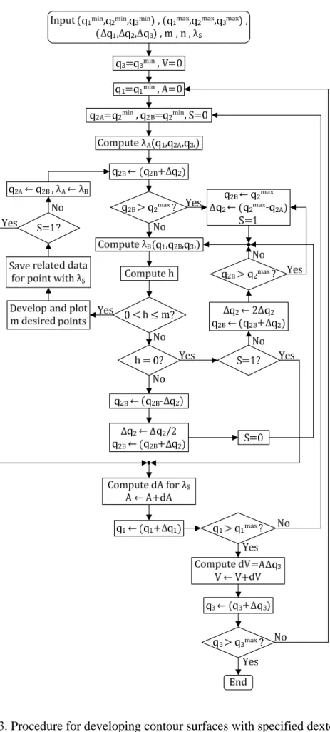
The procedure for developing surfaces with kn

  for k = 1, 2, 3, .., n-1 is shown in Fig.

3. It is easier to study the contour surfaces if surfaces with different  are plotted on different coordinate frame. The algorithm is applicable to general, special, or redundant serial manipulators.

In general, the joint space or task space of a manipulator consists of several groups of contour surfaces, and each group contains a local optimum of . The second algorithm evaluates the dexterity of a particular group of contour surfaces using spherical coordinates defined in Eq. (8). With the local optimum as the origin and the outmost contour surface specified by , the steps_min are given below:

1. Input the origin (with _max and use it as the starting A), joint limits (if they exist), ,  , and number_min n

2. Let  =  and m = g(_max) /n. Determine the minimum integer k such that ^k

n  . Search for _min at the starting orientation with

k

 n and use it as the second point B.

3. Develop points between A and B with k ¹,k ²

n n

 ^ ^ ,….., m n/ using the bisection method.

4. Compute the distance from A to each point obtained. If there is no joint limit, then save the related data and go to Step 6.

5. Compute the joint displacements using Eq. (8) (for the contour surfaces in joint space) or solve the inverse kinematics (for the contour surfaces in task space) for each desired point obtained. Save the related data for points whose joint displacements are all within the related joint limits.

6. Find the next orientation using a

grid-canning approach. Exit if all possible orientations have been searched.

7. Search for  at the new orientation with ^k

 n and use it as the second point B. Go to Step 3.

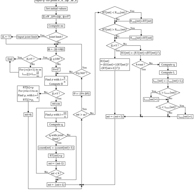
Figure 4 shows the procedure for evaluating the dexterity for a particular group of contour surfaces. In general, the steps on the left-hand side input or set initial data, compute ρ with different λ, and temporarily save the obtained results (in array RT) that are then employed to update the recorded data using the steps at the right-hand side.

With  denoting the length associated with_j λ = j nൗ , R_min[j] and R_max[j] record _jmin (the minimum ) and_j _jmax(the maximum

 ) respectively for j = k, k+1,…., m. R3[j]j

records the summation of ρ_୨^ଷ for manipulators without joint limits. The volume of the region with λ ≥ j nൗ is proportional to R3[j]. The algorithm also investigates the relative positions of two neighboring surfaces. The maximum distance, the minimum distance, and the average distance between two neighboring surfaces with λ = j nൗ and λ = (j − 1) nൗ are saved in L_max[j], L_min[j], and L_ave[j] respectively for j = k+1, k+2, …., m. The initial values for all count[j], RT[j], R_max[j], R3[j], Lmax[j], and L_ave[j] are set to zero, and a very large initial number is assigned to allR_min[j] and Lmin[j].

Since the points with φ = 0ô, φ = 180ô or θ = 360ôare excluded, the number of sample points reached for each λ is ns = ቀ^ଵ଼଴_ο஦^౥− 1ቁ(^ଷ଺଴_ο஘^౥). For manipulators with joint limits, some surfaces might not be reached or only a few points can be reached for a smaller λ.

The relative positions of two neighboring surfaces cannot be determined by the relative positions of a few sample points, so the

(9)

distance between two neighboring surfaces is not considered in this case. The number of points that can reach λ = j nൗ is saved in count[j], and R [j] records (³ _j³_j+1³ ) for j

= k, k+1,…., m with ρ_{୫ ାଵ}= 0. The volume of the region with λ ≥ j nൗ is proportional to

m 3

j= i

R [i]



for manipulators with joint limits.

The algorithm can be employed to develop contour surfaces in joint space or task space.

The vector of joint displacements q can be computed by Eq. (8) or by solving inverse kinematics (for contour surfaces in task space).

The third algorithm also studies a particular group of contour surfaces. More accurate results can be obtained by the algorithm. The algorithm needs an initial point to start with. The point can be any point that belongs to a particular branch of kinematic solution or the point can be used to indicate the region where contour surfaces want to be developed. With the initial point, the first closed curve with ^k

 n on a cross-section can be developed using the points shown in Fig. 1. The coordinates and the number of points obtained are recorded for computing the length of the boundary curve and the area of the enclosed region.

The approach in the second algorithm can be employed (with spherical coordinates replaced by polar coordinates) to develop the rest of contour curves inside the region, but developing the local optimum of λat each cross-section is a rather time-consuming task.

In this work, a point near the center point of the enclosed region is utilized to find the starting point for developing the curve with

k+1.

 n Let N[1], N[2], ….,N[m] denote the points on the curve with ^k

 n. Then the middle point on the curve is N[s] with s

=[^ଵା୫_ଶ െ ቀ^ଵା୫_ଶ ǡͳቁሿ. If λ at the middle

point of N[1] and N[s] is larger than ^k+1 n , then use the point and N[1] to develop the starting point for the curve with ^k+1.

 n Otherwise, compute λ at other middle points of (N[1],N[2]), (N[1],N[3]), …, and (N[1],N[m]) to find the point with optimum λ and use it to develop the starting point for the next curve. Compute the length of the boundary curve and the area of the enclosed region if the number of points obtained m ≧ 3. The steps to develop contour surfaces are summarized below:

1. Input the initial point A₀ = (qଵ଴ǡqଶ଴, qଷ଴), and numbers n and k^* for developing the outmost surface with λ= ^୩_୬^∗. q∗ଷ= qଷ଴. k = k^*. S = 0. Develop the first point P with λ= ^୩_୬.

2. Use point P to develop the close curve with λ= ^୩_୬ . Record the related data. Go to Step 4 If m < 3.

3. Compute the length of the boundary curve and the area of the enclosed region. k = k + 1. Find a point inside the current closed curve with

k

 n. Go to Step 5 if the point cannot be obtained. Use the point and point N[1] (of the current curve) to find a point with ^k

 n. Let the point obtained as point P. Go to Step 2.

4. Go to Step 6 if λ= ^୩_୬^∗.

5. q_ଷ= q_ଷ+ Δq_ଷ. k = k^*. Develop the first point P with λ =^୩_୬ on the cross-section at q3. Go to Step 2.

6. Exit if S = 1. Δq_ଷ= −Δq_ଷ . q_ଷ= q^∗_ଷ+ Δq_ଷ. S = S+1. k = k^*. Develop the first point P with λ =^୩_୬ on the cross-section at q₃. Go to Step 2.

(10)

Some data of one cross-section can be utilized to facilitate the developing process for the curves at the next cross-section. For example, if q_ଵ^∗ and q_ଶ^∗ are the first two coordinates of point P (or point N[1]) on one cross-section, then point (q_ଵ^∗, q^∗_ଶ− Δq_ଶ) and (q∗ଵ, q∗ଶ+ Δqଶ) can be employed in the bisection method to develop the first point P for the curve (with the same λ) on the next cross-section. The tangent vector at point P of one section can be directly used as the tangent vector at point P of the next section.

The procedure of the algorithm is shown in Fig. 5.

This section presents algorithms to develop all contour surfaces or one particular group of contour surfaces with specified dexterities. The first algorithm develops all contour surfaces in the joint space (it can also be used to develop a particular group of surfaces if the ranges for the surfaces are given). The contour surfaces in the task space can be easily developed using direct kinematics. Note that any contour surface in the task space with λ = c (≠ 0) is the boundary of a singularity-free workspace with λ ≥ c. The algorithm is applicable to redundant manipulators.

The second algorithm needs a local optimum of λ to develop a group of contour surfaces that contains the local optimum.

Currently, many isotropic designs can be easily obtained by existing methods. The algorithm can be employed to determine which design has better dexterity. The isotropic configuration can be directly used as the origin of the reference frame. The algorithm is not applicable to redundant manipulators because there might be several local optimums of  that are very close to each others. Except for special manipulators whose inverse kinematics can be solved through equations of degree two, surfaces with fairly small λ might not be simply-connected surfaces that do not belong to a particular group of contour surfaces. In general, those surfaces can be excluded if the input value of λmin (or ^୩^∗

୬) > 0.2 for general manipulators and λmin > 0.5 for redundant

manipulators.

The third algorithm also develops one group of simply-connected contour surfaces.

The approach yields accurate results of the area of a boundary surface and the volume of the enclosed region. The method, however, can only develop continuous surfaces, so it cannot be employed to study manipulators with limited joint ranges.

4. Examples

Example 1: The first algorithm is employed to develop contour surfaces of two 4-DOF redundant isotropic manipulators. The first manipulator with a = 4.3802,₁ d = 1.8892,₁

1 190.5131^o

  , a = 4.7562,₂ d = 2.7281,₂

2 81.769^o

  , a = 2.154,₃ d₃ = 4.5862,

3 190.489^o

  , a₄ = 2.8017, d = 2.6529₄ and ₄ 130.7402^o can reach only one isotropic configuration while the second special design with a1= 2 , a2= a3= 3.7, a4= 2.6, d1 = d2 = d3 = d4 = 0, ₁ 90^o , αଶ= αଷ= αସ= 0 can reach up to 16 isotropic configuration [8]. The surfaces for λ = 0.9, 0.7 and 0.5 are shown in Figs. 6 and 7. Figure 7a shows that there are four similar regions with λ > 0.9. Each region contains four isotropic configurations. The figures show that the second design has much better dexterity, which can verified by the volume for the region with λ≧ 0.7 (the volumes for the two designs are 0.6157 and 6.9288 respectively). If a1 = 1 for the second design, then the manipulator can only reach eight isotropic configurations [8]. In this case, the volume for the region with λ ≧ 0.7 is 4.8982. It seems that isotropic manipulators with more isotropic configurations have better global dexterity.

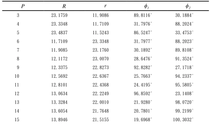
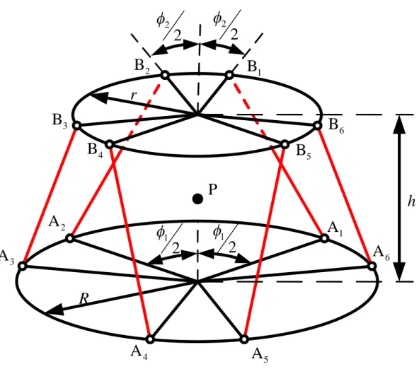
Example 2: Figure 8 and Table 1 show the parameters that define a group of 6-DOF Stewart-Gough parallel manipulators with the same local optimum dexterity at the initial assembly configuration [9]. The second algorithm is employed to find the design with the best dexterity. The dexterity in the orientation space is investigated with

(11)

limited joint ranges _oi 6 _i _oi6 for i = 1, 2, …, 6, where  and_i  denote,_oi respectively, the i^th limb length and the i^th limb length at the initial assembly configuration. The orientation space is specified by Z-Y-Z Euler angles. With the origin of the coordinate frame at the tool center point P, n = 10 and     , the  6^o results are listed in Table 2. The orientation workspace is proportional to the total number of points that can be reached, so the design with P = 6 (which can reach 93 points) has the largest orientation workspace at the initial assembly configuration. The tool center point of the design is inside the manipulator. If the tool center point must be outside a manipulator, then the design with P = 11 is a better choice. The dexterity can be compared by the volumes of the regions with k

  10 for k = 9, 8, …, 5. The design with P = 5 (or the tool center point is near the geometric center of the manipulator) has the best dexterity despite the fact that it can only reach the points with λ ≧ 0.7. The design with P = 11 is the best choice if the tool center point must be outside of a manipulator.

5. Conclusion

The analytical solutions of the cubic and the bisection method have been employed to develop algorithms for evaluating the dexterity of manipulators. The algorithms can be employed to develop all contour surfaces or a particular group of contour surfaces with specified dexterities. The dexterity can be evaluated by the volume enclosed by a closed surface with specified dexterity, and the rate of change of dexterity can be determined by the related positions of the contour surfaces. The methods are applicable to special, general, or redundant manipulators with or without joint limits. The proposed algorithms have been employed to study the dexterity of 4-DOF redundant serial manipulators and the dexterity and orientation workspace of a group of 6-DOF isotropic parallel manipulators. With some

modifications, the algorithms can be extended to evaluate the dexterity of 6-DOF manipulators because the local dexterity at a given configuration can also be evaluated by the solutions of the cubic.

Acknowledgments

Support from the National Science Council of the Republic of China under grant NSC97-2212-E011-051 is gratefully acknowledged.

References

[1] C. A. Klein and B. E. Blaho, “Dexterity measures for the design and control of kinematically redundant manipulators,” Int. J.

Robot. Res. 6(2), 72-83 (1987).

[2] C. Gosselin and J. Angeles, “A global performance index for the kinematic optimization of robotic manipulators,” ASME J. Mech Des, 113(3), 220-226 (1991)

[3] D. Chablat, Ph. Wenger, F. Majou, and J.

P. Merlet, “An interval analysis based study for the design and the comparison of three-degree-of-freedom parallel kinematic machines,” Int. J. Robot. Res. 23(6), 615-624 (2004).

[4] J. P. Merlet, “Jacobian, manipulability, condition number, and accuracy of parallel robots,” ASME J. Mech Des, 128(1), 199-208 (2006)

[5] X.-J. Liu, Z.-L. Jin, and F. Gao,

“Optimum design of 3-DOF spherical parallel manipulators with respect to the conditioning and stiffness indices,” Mech.

Mach. Theory, 35(9), 1257-1267 (2000).

[6] X.-J Liu, J. Wang, and H.-J Zheng,

“Optimum design of the 5R symmetrical parallel manipulator with a surrounded and good-condition workspace,” Robot. Auton.

Syst., 54(3), 221-233 (2006)

[7] K. Y. Tsai and S. R. Zhou, “The optimum design of 6-DOF isotropic parallel manipulators,” J. Robot. Syst, 22(6), 333-340 (2005)

[8] K. Y. Tsai, P. Y. Lin, and T. K. Lee, 2008,

“4R spatial and 5R parallel manipulators that can reach maximum number of isotropic positions” Mech. Mach. Theory, 43(1), 68-79 (2008).。

(12)

[9] K. Y. Tsai, T. K. Lee, and Y. S. Jang, “A new class of isotropic generators for

developing 6-DOF isotropic manipulators,”

Robotica, 26(5), 619-625 (2008)

(13)

Table I Parameters of symmetric generators for h10

P R r ₁ ₂

3 23.1759 11.9086 89.8116° 30.1884°

4 23.3348 11.7109 31.7976° 88.2024°

5 23.4837 11.5243 86.5247° 33.4753°

6 11.7109 23.3348 31.7977° 88.2023°

7 11.9085 23.1760 30.1892° 89.8108°

8 12.1172 23.0070 28.6476° 91.3524°

9 12.3375 22.8273 92.8282° 27.1718°

10 12.5692 22.6367 25.7663° 94.2337°

11 12.8101 22.4368 24.4195° 95.5805°

12 13.0634 22.2249 96.8592° 23.1408°

13 13.3284 22.0010 21.9280° 98.0720°

14 13.6054 21.7648 20.7801° 99.2199°

15 13.8946 21.5155 19.6968° 100.3032°

Table II Related data for orientation workspace and dexterity

P ^V

0.4 0.5 0.6 0.7 0.8 0.9 0.9 0.8 0.7 0.6 0.5 0.4

3 5 7 7 7 9 25 0.4656 0.6765 0.8800 1.1867 1.6385 2.1508 4 nil nil nil ⁷ ^{19 31} 1.4755 2.1690 2.5305 nil nil nil

5 nil nil nil ^{11 31 31} 1.2900 2.5776 3.1447 nil nil nil

6 nil ⁹ ¹⁰ ^{18 25 31} 0.8333 1.3970 1.8574 2.1225 2.4895 nil

7 nil ⁹ ¹¹ ^{13 23 27} 0.1501 0.5812 0.8761 1.2385 1.6789 nil

8 nil ⁸ ¹¹ ^{11 25 31} 0.2275 0.8711 1.1053 1.5553 2.0520 nil

9 nil ⁴ ¹¹ ^{12 29 31} 0.1717 0.9024 1.1953 1.6818 2.0277 nil

10 nil ⁵ ⁸ ^{13 29 29} 0.1300 0.7847 1.2177 1.6946 2.2911 nil

11 nil ² ⁸ ^{22 29 31} 0.1448 0.7544 1.6756 2.1730 2.3599 nil

12 nil nil ⁶ ^{21 31 31} 0.1337 0.6873 1.4391 1.7864 nil nil

13 nil nil ⁴ ^{23 31 31} 0.1519 0.7838 1.6798 1.9632 nil nil

14 nil nil ² ^{16 31 31} 0.1540 0.8428 1.4414 1.5762 nil nil

15 nil nil ² ^{14 29 31} 0.1525 0.7813 1.2787 1.4343 nil nil number of points reached

(14)

1

A

0

A

1

n_i = ൤−t_iy t_ix ൨

Pi

ti

Pi-2

Pi-1

Hi

Qi