Bernoulli-Euler平面剛架中含分佈質量的動力分析法

行政院國家科學委員會專題研究計畫 成果報告

Bernoulli-Euler 平面剛架中含分佈質量的動力分析法 研究成果報告(精簡版)

計 畫 類 別 ： 個別型

計 畫 編 號 ： NSC 97-2221-E-011-068-

執 行 期 間 ： 97 年 08 月 01 日至 98 年 07 月 31 日 執 行 單 位 ： 國立臺灣科技大學營建工程系

計 畫 主 持 人 ： 蔡相全

計畫參與人員： 碩士班研究生-兼任助理人員：周志昇 碩士班研究生-兼任助理人員：周伯融 碩士班研究生-兼任助理人員：方韻喬

處 理 方 式 ： 本計畫涉及專利或其他智慧財產權，2 年後可公開查詢

中 華 民 國 98 年 06 月 02 日

Distributed-Mass Approach for Dynamic Analysis of Bernoulli-Euler Plane Frames

Hsiang-Chuan Tsai

¹

Department of Construction Engineering, National Taiwan University of Science and Technology, Taipei, Taiwan.

Abstract

The exact method for the dynamic analysis of plane frames should consider the effect of mass distribution in beam elements, which can be achieved by using the dynamic stiffness method. The dynamic stiffness matrices of beam elements are derived from the vibration theory of Bernoulli-Euler beams and then assembled by the direct stiffness approach to obtain the dynamic stiffness matrix of the whole plane frame, which is a function of vibration frequency, but cannot be decomposed into static stiffness matrix and mass matrix. Solving natural frequencies and mode shapes of plane frames from the dynamic stiffness matrix is a nonlinear eigenproblem. A deflated matrix method to solve the mode shapes is presented. Numerical approach to find the special modes in which the joints of beam elements are null is also discussed. Orthogonal properties of vibration modes in plane frames considering distributed mass are theoretically derived, through which the equations of motion in beam elements can be transformed into the decoupled equations of motion in terms of mode amplitudes. After solving the transient response of each vibration mode, the mode superposition approach can be applied to calculate frame deformation and element stresses.

Keywords: Bernoulli-Euler beam; Distributed mass; Dynamic stiffness matrix; Plane frame;

Structural dynamics; Wittrick-Williams algorithm.

1. Introduction

Vibration of a beam element can be modeled as a continuous-coordinate system and solved from the differential equation of motion and the related boundary conditions. Vibration of a plane frame, which is an assemblage of beam elements, is usually analyzed by a discrete-coordinate system in which the stiffness matrix is established through the static equilibrium equation of beam elements; the mass matrix may be either formed by lumping the mass at the structural joints, called the lumped-mass method, or computed from the

1

P.O. Box 90-130, Taipei 106, Taiwan. Fax: +8862-27376606. E-mail: [email protected]

static-deformed shape functions of beam elements, called the consistent-mass method. The solutions of the discrete models can only approximate the actual dynamic behavior. Craig (1981) compared the natural frequencies of a uniform cantilever beam calculated by the exact continuous model with the solutions determined by the lumped-mass method and the consistent-mass method, and revealed that the accuracy of the natural frequencies calculated by the discrete models deteriorates in the higher modes. The continuous-model approach utilized in the dynamic analysis of a single beam element is recognized to be not feasible for the dynamic analysis of plane frames because the necessary boundary conditions become unmanageable (Chopra, 1995).

From the differential equation of beam vibration, the relationships between harmonic forces and displacements at the ends of a beam element can be exactly established. These relations are usually referred to as the dynamic stiffness matrix. The elements in the dynamic stiffness matrix are nonlinear functions, trigonometric and hyperbolic, of vibration frequency. By expanding the dynamic stiffness matrix in a Taylor’s series, Paz (1973) demonstrated that the first term of the series, the zero power of frequency, is the static stiffness matrix, and the second term of the series, the second power of frequency, is the consistent mass matrix. After the dynamic stiffness matrices of beam elements are derived, the dynamic stiffness matrix of the whole frame can be assembled by exactly the same procedure used in the static matrix structural analysis. The historical development of using the dynamic stiffness matrix in structural dynamics has been highlighted by Akesson (1976).

The dynamic stiffness matrix, which is frequency-dependent, can be directly employed in solving the steady-state response of the frames subjected to harmonic loadings. To solve the problems of transient response, the natural frequencies and mode shapes of the frames must be first calculated from the dynamic stiffness matrix, which is usually referred to as a nonlinear eigenproblem and is different from the linear eigenproblem encountered in the dynamic analysis of discrete systems. Extending the Sturm sequence property of linear eigenproblems, the Wittrick-Williams algorithm (Williams and Wittrick, 1970; Wittrick and Williams, 1971) can count the number of vibration modes exceeded by a specified frequency from the dynamic stiffness matrix, which ensures that no natural frequencies are missed when using the bisection or other methods (Kennedy and Williams, 1991) to solve the zero determinant equation of the dynamic stiffness matrix.

The orthogonality of vibration modes is the required condition of using the vibration modes to solve the transient response of the frames. The publications on the orthogonality of vibration modes employed in the dynamic stiffness matrix are few and less rigorous (Chan and Williams, 2000). The present paper derives the mode orthogonality condition of the Euler-Bernoulli plane

frame with distributed mass for the modes of different natural frequencies, through which the equations of motion in terms of structural joints deformation can be transformed into the decoupled equations of motion in terms of vibration mode amplitudes. Not every vibration mode has distinct natural frequency. Sometimes several modes may have the same natural frequency, which are called the modes of repeated roots. The decoupling process for the modes of repeated roots is also derived in this paper.

There are several methods to solve the mode shapes from the dynamic stiffness matrix (Hopper and Williams, 1977) which, however, have been evaluated as being not very stable (Yuan, Ye and Williams, 2004). A deflated matrix approach to solve the mode shapes from the dynamic stiffness matrix is proposed in this paper, which is then extended to find the orthogonal mode shapes of the repeated-root modes. In the vibration of frames considering the effect of distributed mass, a special type of vibration modes may occur where the deformations at all frame joints are null but the deformations in beam elements are not null, which is called the null modes here. The null mode shapes cannot be directly solved from the dynamic stiffness matrix.

Efficient approach to find the mode shapes of null modes is also discussed in this paper.

2. Flexural dynamic stiffness of beam elements

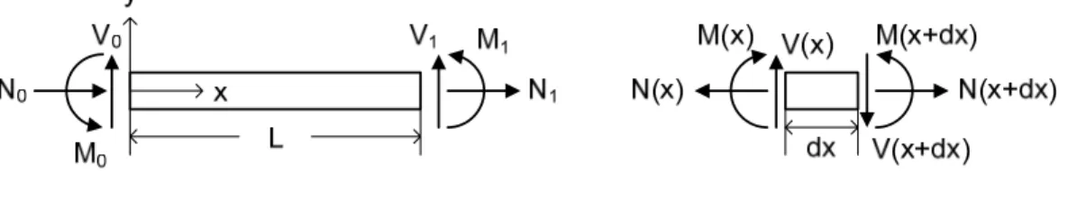
The prismatic beam element shown in Fig. 1 has length L, cross-sectional area A, moment of area I, Young’s modulus E, and density ρ . The x axis is the coordinate along the beam axis. Let

v denote the transverse displacement of the beam in the y direction. The equation of motion for

the transverse free vibration of the Bernoulli-Euler beam is

2 0

2 4

4 =

∂ + ∂

∂

∂

t A v x

EI v ρ

(1)

with time t. When the beam is vibrating at a specific frequency

ω

, the transverse displacement can be expressed as

t

e

i

x t

x

v

( , )=

ψ

( ) ^ω (2)

in which ψ is the transverse shape function. Eq. (1) becomes

4 0

4

4

ψ

−

β ψ

=

x d

d

(3)

where

ω ρ

β

=⁴ (

A

) (

EI

) (4)

The solution of ψ in Eq. (3) has a form as

x b

x b

x b

x b

x β β β β

ψ

( )= ₁cos + ₂sin + ₃cosh + ₄sinh (5)

in which the constants can be determined from the transverse displacements and slopes at the beam ends,

b

i

⎪⎪

⎭

⎪⎪

⎬

⎫

⎪⎪

⎩

⎪⎪

⎨

⎧

′

′

⎥⎥

⎥⎥

⎦

⎤

⎢⎢

⎢⎢

⎣

⎡

− +

−

−

−

−

−

−

− +

=

⎪⎪

⎭

⎪⎪

⎬

⎫

⎪⎪

⎩

⎪⎪

⎨

⎧

) (

) (

) 0 (

) 0 (

) (

) (

2 1

6 4 3

0 1

5 6 2

3 0

6 4 3

0 1

5 6 2

3 0

0 4

3 2 1

L L B

B B

B B

B B B

B B

B B B

B B

B B B

B B

B b

b b b

ψ ψ ψ ψ

β β

β β

β β

β β

(6)

with

L L

B

₀ =1−cos

β

cosh

β

L L

L L

B

₁=sin

β

cosh

β

+cos

β

sinh

β L L

L L

B

₂ =sin

β

cosh

β

−cos

β

sinh

β L

L B

₃ =sin

β

sinh

β

L L

B

₄ =sinh

β

+sin

β

L L

B

₅ =sinh

β

−sin

β L L

B

₆ =cosh

β

−cos

β

The bending moment M and the shear force V in the prismatic Bernoulli-Euler beam have the following relations with the transverse displacement,

) ( )

( x EI x

M =

ψ

′′

;

V ( x ) = EI

ψ

′′′ ( x )

(7)

Let

M

₀,

V

₀,

ψ

₀ and

θ

₀ denote the bending moment, shear force, transverse displacement and slope, respectively, at the beam end of

x

=0, and

M

₁ ,

V

₁,

ψ

₁ and

θ

₁ be the corresponding quantities at the beam end of

x

= . The positive directions of the end forces and

L

internal forces are shown in Fig. 1, which give the relations

) 0

0

M

(

M

=− ;

V

₀ =

V

(0) ;

ψ

₀ =

ψ

(0) ;

θ

₀ =

ψ

′(0) (8) )

1

M

(

L

M

= ;

V

₁ =−

V

(

L

) ;

ψ

₁=

ψ

(

L

) ;

θ

₁=

ψ

^′(

L

) (9) Substituting Eq. (5) into Eq. (7) and using the relations in Eqs. (8) and (9), the flexural dynamic

stiffness of the Bernoulli-Euler beam is derived as

⎪⎪

⎭

⎪⎪

⎬

⎫

⎪⎪

⎩

⎪⎪

⎨

⎧

⎥⎥

⎥⎥

⎥

⎦

⎤

⎢⎢

⎢⎢

⎢

⎣

⎡

−

−

−

−

−

−

=

⎪⎪

⎭

⎪⎪

⎬

⎫

⎪⎪

⎩

⎪⎪

⎨

⎧

1 1 0 0

2 3

2 5

6 2

3 2 1 3 6

2 4 3

5 6

2 2 3

2

6 2 4 3 3 2 1 3

0 1 1

0 0

θ ψ θ ψ

β β

β β

β β

β β

β β

β β

β β

β β

B B

B B

B B

B B

B B

B B

B B

B B

B EI

M V M V

(10)

3. Complete dynamic stiffness of beam elements

In order to be able to robotically form the dynamic stiffness of the frame, the axial stiffness

must be included in the dynamic stiffness of beam elements. Let u denote the axial displacement of the beam in the x direction. The equation of motion for the axial free vibration is

2 0

2 2

2 =

∂ + ∂

∂

− ∂

t A u x

EA u ρ

(11)

When the beam is vibrating at a specific frequency

ω

, the axial displacement can be expressed as

t

e

i

x t

x

u

( , )=

χ

( ) ^ω (12)

in which χ is the axial shape function. Eq. (11) becomes

2 0

2

2

χ

+

α χ

=

x d

d

(13)

where

) ( ) (

ρ A EA ω

α

= (14)

The solution of χ in Eq. (13) has a form as

x

a x a

x α α

χ

( )= ₁cos + ₂sin (15)

in which the constants

a

_i can be determined from the axial displacement at the beam ends,

⎭⎬

⎫

⎩⎨

⎥⎧

⎦

⎢ ⎤

⎣

⎡

= −

⎭⎬

⎫

⎩⎨

⎧

) (

) 0 ( sin

1 tan 1

0 1

2 1

L L a L

a

χ χ α

α

⁽¹⁶⁾

The axial force N in the prismatic beam has the following relation with the axial displacement,

) ( )

( x EA x

N =

χ

′

(17)

Let

N

₀ and

χ

₀ denote the axial force and axial displacement, respectively, at the beam end of , and and

=0

x N

₁

χ

₁ be the corresponding quantities at the beam end of . The positive directions of the end forces and internal forces in Fig. 1 give the relations

L x

=

) 0

0

N

(

N

=− ;

χ

₀ =

χ

(0) ;

N

₁=

N

(

L

) ;

χ

₁ =

χ

(

L

) (18) Substituting Eq. (15) into Eq. (17) and using the relations in Eq. (18), the axial dynamic stiffness

is derived as

⎭⎬

⎫

⎩⎨

⎥⎧

⎦

⎢ ⎤

⎣

⎡

−

= −

⎭⎬

⎫

⎩⎨

⎧

1 0 1

0

cos 1

1 cos

sin

χ

χ α α

α α

L L

L EA N

N

(19)

The complete dynamic stiffness of the Bernoulli-Euler beam can be obtained by combining Eqs. (10) and (19),

⎪ ⎪

⎪ ⎪

⎭

⎪⎪

⎪ ⎪

⎬

⎫

⎪ ⎪

⎪ ⎪

⎩

⎪⎪

⎪ ⎪

⎨

⎧

⎥ ⎥

⎥ ⎥

⎥ ⎥

⎥ ⎥

⎥ ⎥

⎥ ⎥

⎥ ⎥

⎥

⎦

⎤

⎢ ⎢

⎢ ⎢

⎢ ⎢

⎢ ⎢

⎢ ⎢

⎢ ⎢

⎢ ⎢

⎢

⎣

⎡

−

−

−

−

−

−

−

−

=

⎪ ⎪

⎪ ⎪

⎭

⎪⎪ ⎪

⎪

⎬

⎫

⎪ ⎪

⎪ ⎪

⎩

⎪⎪ ⎪

⎪

⎨

⎧

1 1 1 0 0 0

0 2 0

3 2

0 5 0

6 2

0 3 2

0 1 3

0 6 2

0 4 3

0 5 0

6 2

0 2 0

3 2

0 6 2

0 4 3

0 3 2

0 1 3

1 1

1 0 0

0

0 0

0 0

0 tan 0

0 sin 0

0 0

0 0

0 sin 0

0 tan 0

θ ψ χ θ ψ χ

β β

β β

β β

β

β α

α α

α

β β

β β

β β

β

β α

α α

α

B B B

B B

B B

B

B B B

B B

B B

B

L I

A L

I A

B B B

B B

B B

B

B B B

B B

B B

B

L I

A L

I A

EI

M V N M V N

(20)

4. Dynamic stiffness of plane frames

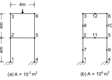
The plane frame shown in Fig. 2 is defined by a global coordinate system

( x , y )

. Let

u ,

_i

v

_i and θ denote the displacements in the _i

x

and y directions and the rotation, respectively, at joint i. The total number of the unconstrained degrees of freedom in the joints of the frame is denoted as

n

_d. The beam element J has two ends at joints i and j. Let

X

_i,

Y

_i and

M

_i denote the forces in the

x

and y directions and the moment, respectively, acting at the joint i of the element J. The transformation between the element local coordinates and the frame global coordinates gives

⎪⎭

⎪⎬

⎫

⎪⎩

⎪⎨

⎧

⎪=

⎭

⎪⎬

⎫

⎪⎩

⎪⎨

⎧

i i i

v u

θ θ

ψ χ

T

0 0 0

;

⎪

⎭

⎪ ⎬

⎫

⎪ ⎩

⎪ ⎨

⎧

⎪ =

⎭

⎪ ⎬

⎫

⎪ ⎩

⎪ ⎨

⎧

j j j

v u

θ θ

ψ χ

T

1 1 1

;

⎪

⎭

⎪ ⎬

⎫

⎪ ⎩

⎪ ⎨

⎧

⎪ =

⎭

⎪ ⎬

⎫

⎪ ⎩

⎪ ⎨

⎧

i i

i

M Y X

M V N

T

0 0

0

;

⎪

⎭

⎪ ⎬

⎫

⎪ ⎩

⎪ ⎨

⎧

⎪ =

⎭

⎪ ⎬

⎫

⎪ ⎩

⎪ ⎨

⎧

j j

j

M Y X

M V N

T

1 1

1

(21)

where

T

is the transformation matrix defined as

⎥ ⎥

⎥

⎦

⎤

⎢ ⎢

⎢

⎣

⎡

−

−

−

−

−

=

1 0

0

0 ) (

) (

0 ) (

) (

L x x L y y

L y y L x x

i j i

j

i j i

j

T

(22)

with (

x

_i,

y

_i) being the coordinates of the joint i. The element length L can be calculated by

2

2 ( )

)

(

x

_j

x

_i

y

_j

y

_i

L

= − + − (23)

The dynamic stiffness matrix in Eq. (20) can be transformed to the element stiffness matrix in the global coordinate system by using Eq. (21). The global stiffness matrices of all elements in the frame are then assembled to form the frame stiffness matrix

K (

ω

)

by means of the direct stiffness method, which yields

0 d

K (

ω

) =

(24)

in which

K (

ω

)

is a matrix and is a function of frequency, and is the displacement vector of the unconstrained degrees of freedom in the joints of the frame. Without any external force, the summation of the internal nodal forces leads to the zero vector at the right side. The natural frequencies and shape vectors of the vibration modes can be solved from Eq. (24), which will be studied later.

d

d

n

n

×

d

5. Orthogonality of mode shape functions

After the nth mode shape vector of the frame being solved, the transverse and axial shape functions of element J in the nth mode,

d

n

ψ

Jn and

χ

_Jn respectively, can be derived from Eqs. (5) and (15). Similar to Eqs. (1) and (11), the equations of motion for element J vibrating in the nth mode with natural frequency

ω

_n are

0 )

( )

( ₄ ²

4 − _{J n Jn} =

J Jn

J

A

x d

EI d ψ ρ ω ψ

(25)

0 )

( )

(

₂ ²

2

− =

−

_{J n Jn}

J Jn

J

A

x d

EA d

χ ρ ω χ

(26) in which (

EI )

_J, (

EA)

_J, (

ρ A)

_J and are the flexural stiffness, axial stiffness, mass per unit

length, and axial coordinate of element J, respectively. Multiply Eqs. (25) and (26) by the transverse and axial shape functions of element J in the mth mode, respectively, and then integrate the summation of the two equations through the element length . Summing the integrations of all elements up leads to

x

J

L

J

[ ] [ ]

{ ^{( ) ( ) ( ) ( )} } ⁰

0

2

2

− ′′ + =

∑∫ −

J L

J Jn n J Jn

J Jm Jn n J IV

Jn J Jm

J ψ

EI

ψ ρ

A

ωψ χ

EA

χ ρ

A

ω χ

dx

(27)

which becomes, through integration by part,

{ }

∑

∑∫

′ + +

−

= +

′ − + ′

′′

′′

J

L Jn Jm Jn Jm Jn Jm J

L

J Jn Jm Jn Jm J n Jn Jm J Jn

Jm J

J J

N M

V

dx A

EA EI

0 0

2

) (

) (

) ( )

( )

(

χ ψ

ψ

χ χ ψ ψ ρ ω χ χ ψ

ψ

(28)

The right side of Eq. (28) can be expressed in vector form by using the notations similar to

Eqs. (8), (9) and (18),

∑

∑ ⎟⎟

⎟ ⎟

⎠

⎞

⎜⎜

⎜ ⎜

⎝

⎛

⎪ ⎭

⎪ ⎬

⎫

⎪ ⎩

⎪ ⎨

⎧

⎪ ⎭

⎪ ⎬

⎫

⎪ ⎩

⎪ ⎨

⎧

⎪ +

⎭

⎪ ⎬

⎫

⎪ ⎩

⎪ ⎨

⎧

⎪ ⎭

⎪ ⎬

⎫

⎪ ⎩

⎪ ⎨

⎧

=

′ + +

−

J

Jn Jn

Jn T

Jm Jm Jm

Jn Jn

Jn T

Jm Jm Jm

J

L Jn Jm Jn Jm Jn Jm

M V N

M V N N

M

V

^J

) (

) (

) (

) (

) (

) (

) (

) (

) (

) (

) (

) ( )

(

0 0

0

0 0 0

1 1

1

1 1 1

0 θ

ψ χ θ

ψ χ χ

ψ

ψ (29)

The coordinate transformation in Eq. (21) gives

⎪ ⎭

⎪ ⎬

⎫

⎪ ⎩

⎪ ⎨

⎧

⎪ ⎭

⎪ ⎬

⎫

⎪ ⎩

⎪ ⎨

⎧

⎪ =

⎭

⎪ ⎬

⎫

⎪ ⎩

⎪ ⎨

⎧

⎪ ⎭

⎪ ⎬

⎫

⎪ ⎩

⎪ ⎨

⎧

⎪ =

⎭

⎪ ⎬

⎫

⎪ ⎩

⎪ ⎨

⎧

⎪ ⎭

⎪ ⎬

⎫

⎪ ⎩

⎪ ⎨

⎧

Jn i

Jn i

Jn i T

m i

m i

m i

Jn i

Jn i

Jn i T T

m i

m i

m i

Jn Jn

Jn T

Jm Jm Jm

M Y X v

u

M Y X v

u

M V N

) (

) (

) (

) (

) (

) (

) (

) (

) (

) (

) (

) (

) (

) (

) (

) (

) (

) (

0 0

0

0 0 0

θ θ

θ ψ χ

T

T

(30)

which means

0 )

( ) (

) (

) (

) (

) (

) (

) (

) (

) (

) (

) (

) (

) (

) (

) (

) (

) (

0 0

0

0 0 0

1 1

1

1 1 1

=

⎟⎟

⎟ ⎟

⎠

⎞

⎜⎜

⎜ ⎜

⎝

⎛

⎪ ⎭

⎪ ⎬

⎫

⎪ ⎩

⎪ ⎨

⎧

⎪ ⎭

⎪ ⎬

⎫

⎪ ⎩

⎪ ⎨

⎧

=

⎟⎟

⎟ ⎟

⎠

⎞

⎜⎜

⎜ ⎜

⎝

⎛

⎪ ⎭

⎪ ⎬

⎫

⎪ ⎩

⎪ ⎨

⎧

⎪ ⎭

⎪ ⎬

⎫

⎪ ⎩

⎪ ⎨

⎧

⎪ +

⎭

⎪ ⎬

⎫

⎪ ⎩

⎪ ⎨

⎧

⎪ ⎭

⎪ ⎬

⎫

⎪ ⎩

⎪ ⎨

⎧ ∑ ∑

∑

i J

Jn i

Jn i

Jn i T

m i

m i

m i

J

Jn Jn

Jn T

Jm Jm Jm

Jn Jn

Jn T

Jm Jm Jm

M Y X v

u

M V N

M V N

θ θ

ψ χ θ

ψ χ

(31)

Without any external force acting at node i, the internal end forces of all the elements connecting to node i are in balance, which leads to zero in the above equation. Using Eq. (31), Eq. (28) becomes

{ ^{( ) ( ) ( ) ( )} } ⁰

0

2

+ =

′ − + ′

′′

∑∫ ′′

J L

J Jn Jm Jn Jm J n Jn Jm J Jn

Jm J

J

EI

ψ ψ

EA

χ χ ω ρ

A

ψ ψ χ χ

dx

(32)

Multiplying the equations of transverse and axial motions of element J vibrating in the mth mode by the transverse and axial shape functions of element J in the nth mode, respectively, the following equation can be established

[ ] [ ]

{ ^{( ) ( ) ( ) ( )} } ⁰

0

2

2

− ′′ + =

∑∫ −

J L

J Jm m J Jm

J Jn Jm m J IV

Jm J Jn

J ψ

EI

ψ ρ

A

ω ψ χ

EA

χ ρ

A

ω χ

dx

(33)

Using the similar procedure described in the last paragraph, the following equation is derived

{ ^{( ) ( ) ( ) ( )} } ⁰

0

2

+ =

′ − + ′

′′

∑∫ ′′

J L

J Jm Jn Jm Jn J m Jm Jn J Jm

Jn J

J

EI

ψ ψ

EA

χ χ ω ρ

A

ψ ψ χ χ

dx

(34)

Subtracting Eq. (32) from Eq. (34) gives the following mass-related orthogonal equation of mode shapes,

0 ) (

)

(

0

∑ ∫ ^{+ =}

J

L

J Jn Jm Jn Jm J

J

dx

A

ψ ψ χ χ

ρ for

ω

_m≠

ω

_n (35)

The stiffness-related orthogonal equation is derived by substituting Eq. (35) into Eq. (32),

{

( ) ( ) 0

0

′′ ′′ + ′ ′ =

∑∫

J L

J Jn Jm J Jn

Jm J

J

EI

ψ ψ

EA

χ χ }

dx

for

ω

_m≠

ω

_n (36)

Bringing in Eq. (35), Eq. (27) gives another form of the stiffness-related orthogonal equation

{ ^{( ) ( ) 0}

0

− ′′ =

∑∫

J L

J Jn Jm J IV

Jn Jm J

J

EI

ψ ψ

EA

χ χ

} dx

^for

ω

m≠

ω

n (37)

By setting

m

=

n

in Eq. (27), the natural frequency and mode shape has the relation as

∑∫

∑∫ ^{− ′′ = +}

J L

J Jn Jn J n

J L

J Jn Jn J IV

Jn Jn J

J

J

EI EA dx A dx

0

2 2 2

0

[( )

ψ ψ

( )

χ χ

]

ω

(

ρ

) (

ψ χ

)

(38)

6. Equations of motion for generalized coordinates

The damping property of the frame can be described through two parameters, ζ and η , where ζ is the stiffness-related viscous damping ratio and η is the mass-related viscous damping ratio. When element J is subjected to distributed loads in the axial and transverse directions, denoted as and , respectively, as shown in Fig. 2, the equations of motion for element J with viscous damping are

f

J

g

_J

) , ( )

( )

( ₂

2 4

5 4

4

t x t g

v t

A v t

x v x

EI v

_J ^{J J} _{J J}

J J

J J

J ⎟⎟⎠=

⎜⎜ ⎞

⎝

⎛

∂ + ∂

∂ + ∂

⎟⎟⎠

⎜⎜ ⎞

⎝

⎛

∂

∂ + ∂

∂

∂

ζ ρ η

(39)

) , ( )

( )

( ₂

2 2

3 2

2

t x t f

u t

A u t

x u x

EA u

_J ^{J J} _{J J}

J J

J J

J ⎟⎟⎠=

⎜⎜ ⎞

⎝

⎛

∂ + ∂

∂ + ∂

⎟⎟⎠

⎜⎜ ⎞

⎝

⎛

∂

∂ + ∂

∂

− ∂

ζ ρ η

(40)

The displacements of force vibration can be expressed as the linear combination of all mode shapes

∑

^∞

=

=

1

) ( ) ( )

, (

k

k J Jk J

J

x t x q t

v

ψ (41)

∑

^∞

=

=

1

) ( ) ( )

, (

k

k J Jk J

J

x t x q t

u

χ (42)

in which the generalized coordinate represents the amplitude of the kth mode. If the frame has a virtual displacement as the nth mode shape, the theory of virtual work gives

q

k

[ ]

[ ]

∑∫ ∑

∑∫ ∑

∑∫ ∑

+ +

+ +

= +

+

′′ +

− +

+ +

+

∞

=

∞

=

i

i n i yi n i xi n i J

L

J J Jn J Jn J

L

J k

k k Jk J k

k Jk J Jn

J L

J k

k k Jk J k

k IV Jk J Jn

Q P

v P u dx

f g

dx q q A

q q EA

dx q q A

q q EI

J J

J

] ) ( )

( ) [(

) (

) (

) ( ) (

) (

) (

) ( ) (

) (

0

0 1

0 1

θ χ

ψ

η χ

ρ ζ

χ χ

η ψ

ρ ζ

ψ ψ

&

&&

&

&

&&

&

(43)

in which

P

_xi,

P and

_yi

Q

_i are the horizontal force, vertical force and moment, respectively, externally acting at node i as shown in Fig. 2, and (

u )

_{i n}, (

v )

_{i n} and

(

θ are the displacements _i

)

_n in the

x

and y directions and the rotation at node i, respectively, of the nth mode shape.

If the nth mode is single root, i.e.

ω

_n ≠

ω

_k for

n ≠ k

, Eq. (43) can be decoupled by using the orthogonal conditions in Eqs. (35) and (37),

) ( ) (

) (

) (

) (

] )

( )

[(

0

2 2 0

t p q q dx A

q q dx EA

EI

n n n J

L

J Jn Jn J

n n J

L

J Jn Jn J IV

Jn Jn J

J J

=

⎭ +

⎬⎫

⎩⎨

⎧ +

+

⎭ +

⎬⎫

⎩⎨

⎧ − ′′

∑∫

∑∫

&

&&

&

η χ

ψ ρ

ζ χ

χ ψ

ψ

(44)

in which

p

_n is the generalized force of the nth mode defined as

∑∫ ^{+ +} ∑ ^{+ +}

=

i

i n i yi n i xi n i J

L

J J Jn J Jn

n

t g f dx u P v P Q

p ( )

^J

( ) [( ) ( ) ( ) ]

0 ψ χ θ (45)

By using Eq. (38), Eq. (44) can be simplified as

nn n n n n n

n

m

t q p

q

q ( )

)

( +

²

+

²

=

+

η ω ζ

_&

ω

&&

(46)

with

∑∫ ⁺

=

J L

J Jn Jn J nn

J

A dx

m

0

2

2

)

( )

(

ρ ψ χ (47)

The solution of the mode amplitude in Eq. (46) is a Duhamel integral.

7. Vibration modes of repeated roots

The equation of motion in Eq. (46) is derived for the modes of single root. For the modes of repeated roots, Eq. (43) cannot be decoupled. Let the modes between the cth mode and the dth mode be the repeated-root mode and have the same frequency ω . Using the orthogonal _c conditions in Eqs. (35) and (37), Eq. (43) gives, for

c

≤

n

≤

d

,

[ ]

[ ^{( ) ( ) ( ) ( )} ] ^{( )}

) (

) ( ) (

) (

0 0

t p dx q q A

q q EA

dx q q A

q q EI

n J

L

J d

c k

k k Jk J k

k Jk J Jn

J L

J d

c k

k k Jk J k

k IV Jk J Jn

J J

= +

+

′′ +

− +

+ +

+

∑∫ ∑

∑∫ ∑

=

=

&

&&

&

&

&&

&

η χ

ρ ζ

χ χ

η ψ

ρ ζ

ψ ψ

(48)

which can be rearranged as

[ ]

) ( ) (

) (

) (

) (

) ( )

(

0 0

t p q q dx A

q q dx EA

EI

n d

c k

k k J

L

J Jk Jn Jk Jn J

d

c k

k k J

L

J Jk Jn J IV

Jk Jn J

J J

= + +

+

′′ +

−

∑∑ ∫

∑∑∫

=

=

&

&&

&

η χ

χ ψ ψ ρ

ζ χ

χ ψ

ψ

(49)

From Eq. (27), we have

[ ] ∑ ∫ [

∑∫ ^{− ′′ = +}

J

L

J Jk Jn Jk Jn J

k J

L

J Jk Jn J IV

Jk Jn J

J

J

EI EA dx A dx

0 2

0

( )

ψ ψ

( )

χ χ ω

(

ρ

)

ψ ψ χ χ

]

⁽⁵⁰⁾

The substitution of Eq. (50) into Eq. (49) yields, for

c

≤

n

≤

d

,

) ( ] )

( [ ) (

)

(

^{2 2}

0

dx q q q p t

A

_n

d

c k

k c k c k

J

L

J Jk Jn Jk Jn J

J

+ + + + =

∑∑

₌ ^ρ

∫

^{ψ ψ χ χ}

^&&

^{η ω ζ}

^&

^{ω (51)}

which can be expressed in the matrix form

⎪ ⎭

⎪ ⎬

⎫

⎪ ⎩

⎪ ⎨

⎧

⎪ =

⎭

⎪ ⎬

⎫

⎪ ⎩

⎪ ⎨

⎧

+ +

+

+ +

+

⎥ ⎥

⎥

⎦

⎤

⎢ ⎢

⎢

⎣

⎡

) (

) (

) (

) (

2 2

2 2

t p

t p

q q

q

q q

q

m m

m m

d c

d c d c d

c c c c c

dd dc

cd cc

M

&

&&

M

&

&&

L M O M

L

ω ζ

ω η

ω ζ

ω η

(52)

with

∑∫ ⁺

=

J L

J Jk Jn Jk Jn J nk

J

A dx

m

0

(

ρ

) (

ψ ψ χ χ

)

(53)

The equations of motion for the repeated-root generalized coordinates can be decoupled as

⎪⎭

⎪⎬

⎫

⎪⎩

⎪⎨

⎧

⎥⎥

⎥

⎦

⎤

⎢⎢

⎢

⎣

⎡

⎪=

⎭

⎪⎬

⎫

⎪⎩

⎪⎨

⎧

+ +

+

+ +

+ ⁻

) (

) ( )

(

)

( ¹

2 2

2 2

t p

t p

m m

m m

q q

q

q q

q

d c

dd dc

cd cc

d c d c d

c c c c c

M L

M O M

L

&

&&

M

&

&&

ω ζ

ω η

ω ζ

ω η

(54)

If the mode shapes that span the space of the repeated-root mode are orthogonal to each other, the magnitudes of

m

_nk become negligible for

n

≠ .

k

8. Solution of natural frequencies

The dynamic stiffness matrix of beam elements has a characteristic of being infinitive at particular frequencies. The flexural dynamic stiffness in Eq. (6) becomes infinitive when

0 cosh cos

1 )

0( = −

L L

=

B ω β β

(55)

For a single beam having both ends clamped, i.e., ψ

( 0 ) =

ψ

( L ) =

ψ

′ ( 0 ) =

ψ

′ ( L ) = 0

, to have a nontrivial shape function defined in Eq. (5), Eq. (55) must be fulfilled. In other words, the frequencies solved from Eq. (55) are the natural frequencies of flexural vibration in a single clamped-clamped beam, which will be called flexural poles here. The nth solution of Eq. (55),

)

( x

ψ

ω

bn, can be solved approximately by

1 as

0 cosh

/ 1

cos

β

L =

β

L ≈

β

L >>

(56)

which gives

A EI n L

bn

ρ

+ π

≈

ω )

² ₂²

2

( 1

(57)

Similarly, the axial dynamic stiffness in Eq. (19) becomes infinitive when 0

sin )

0( =

L

=

A ω α

(58)

For a single beam having both ends fixed in the axial direction, i.e., χ

( 0 ) =

χ

( L ) = 0

, the shape function in Eq. (15) becomes

x a

x α

χ

( )= ₂sin (59)

To have a nontrivial shape function, Eq. (58) must be fulfilled. In other words, the frequencies solved from Eq. (58) are the natural frequencies of axial vibration in a single beam without axial displacement at ends, which will be called axial poles here. The nth solution of Eq. (58),

ω

_an, is

A EA n L

an ρ

ω

=

π (60)

Difficulty in finding the natural frequencies of frames from Eq. (24) arises from the existence of element poles, but can be overcome by using the Wittrick-Williams algorithm (Williams and Wittrick, 1970; Wittrick and Williams, 1971). The algorithm states that

n

_f

(

ω

)

, the total number of natural frequencies in a frame below a specific frequency

ω

, is given by

)}

( { ) ( )

(

ω

n

ω

s K

ω

n

_f

=

_p

+

(61)

where

n

_p

(

ω

)

is the total number of axial and flexural poles in all elements of the frame below the frequency

ω

, and

s { K (

ω

)}

, the sign count of

K (

ω

)

, is the number of negative pivots in the diagonal matrix of pivots

D

after

K (

ω

)

is factorized as

LDL

T

K

(

ω

)= (62)

in which

L

is a lower triangular matrix with all diagonal elements being unity.

By means of the bisection search method or other efficient methods (Kennedy and Williams, 1991), the natural frequencies of the frame can be numerically solved from the determinant of the frame dynamic stiffness matrix

0 )

( det

1

=

=

∏

= nd

i

D

ii

ω

K

(63)