COLLISION AVOIDANCE BY A MODIFIED LEAST-MEAN-SQUARE-ERROR CLASSIFICATION SCHEME FOR INDOOR AUTONOMOUS LAND VEHICLE NAVIGATION

Least-Mean-Square-Error Classification

Scheme for Indoor Autonomous Land

Vehicle Navigation

Ling-Ling Wang

lnstitute of Computer Science and Information Engineering National Chiao Tung University

Hsinchu, Taiwain 30050 Republic of China Wen-Hsiang Tsai*

Department of Computer and Information Science National Chiao Tung University

Hsinchu, Taiwan 30050 Republic of China

Received May 17, 1990; accepted October 29, 1990

In this article, a new collision-avoidance scheme is proposed for autonomous land vehicle (ALV) navigation in indoor corridors. The goal is to conduct indoor collision- free navigation of a three-wheel ALV among static obstacles with no a priori position information as well as moving obstacles with unknown trajectories. Based on the pre- dicted positions of obstacles, a local collision-free path is computed by the use of a modified version of the least-mean-square-error (LMSE) classifier in pattern recogni- tion. Wall and obstacle boundaries are sampled as a set of 2D coordinates, which are then viewed as feature points. Different weights are assigned to different feature points according to the distances of the feature points to the ALV location to reflect the locality of path planning. The trajectory of each obstacle is predicted by a real-time LMSE estimation method. And the maneuvering board technique used for nautical navigation is employed to determine the speed of the ALV for each navigation cycle. Smooth collision-free paths found in the simulation results are presented to show the feasibility of the proposed approach.

*To whom all correspondence should be sent. Journal of Robotic Systems 8(5), 677-698 (1991).

678

Journal of Robotic Systems-1 991

1. INTRODUCTION

Research and development of autonomous land vehicles (ALVs) have re- cently attracted widespread interest. l4 Planning a collision-free path is one of

the fundamental requirements for ALV navigation. Many previous works were concerned with methods for generating a path in a known environment5-I0 or among unknown static

obstacle^.'^-'^

However, obstacles are not always static. Some studies deal with path planning among obstacles that move along known t r a j e ~ t o r i e s . ' ~ , ~ ~ In a real situation, an ALV may face unexpected moving obsta- cles such as human beings. Failure to consider possible intrusion of previously unknown moving obstacles prohibits flexible ALV navigation.

There exist several techniques for path planning in the presence of unknown moving obstacles. Tychonievich et al. l6 extended the maneuvering board

method commonly used for nautical navigation to find a collision-free path through a field of moving obstacles, from a starting point to a goal point, where the goal point can itself be in motion. It is assumed that the instantaneous velocities and positions of the obstacles are known in advance but may be uncertain. Kehtarnavaz and Li" introduced an estimation approach to predict the future positions of obstacles using an autoregressive model. For each obsta- cle, a collision region around the obstacle path from its current position to the predicted position is defined. By drawing tangent lines between these regions, the shortest collision-free path between the current and a desired location of

the vehicle can be obtained. Steele and StarrI8 decomposed the path planning process of a robot into two supporting processes: (1) using a graph search method to plan a path for avoiding all known static obstacles, and (2) using a field potential approach to control the motion of the robot when unexpected obstacles are encountered.

Static obstacles with no a priovi position information, as well as moving obstacles with unknown trajectories, are considered in this study for ALV navigation. The goal is to achieve obstacle avoidance in a corridor. The global path for normal ALV navigation in a corridor is assumed to be known in advance. But the corridor environment might change due to obstacle intrusion '

in every navigation cycle. Therefore, a local navigation path should be recalcu- lated in every navigation cycle. The obstacles, both static (e.g., walls) and moving (e.g., human beings), and the corridor walls are sensed as sets of sampled 2D points. The trajectories of moving obstacles are first predicted by a

real-time LMSE estimation algorithm. I9 A local collision-free navigation path

for an ALV is then computed by a modified version of the LMSE classifier in pattern recognition.20 Different weights are assigned to different 2D points according to the distances of the points to the ALV to emphasize the locality of path planning, and the speed value of the ALV is determined by the maneuver- ing board technique used for nautical navigation. l6 Integration of the three

techniques provides a simple, fast, and intuitive approach to collision avoid- ance for local path planning.

In the remainder of this article, the LMSE classification method used for classifying patterns in pattern recognition, and the modified version of it for guiding an ALV in an obstacle-free corridor, are introduced in section 2. In section 3, the modified LMSE classification method is applied to ALV naviga- tion in a corridor with unknown moving or static obsiacles. The trajectory prediction of the obstacles and the speed control of the ALV for obstacle avoidance are also described. Simulation results are presented in both sections. Conclusions appear in the last section.

2. ALV NAVIGATION I N A CORRIDOR BY A MODIFIED LMSE CLASSIFICATION SCHEME

The LMSE classification method used in pattern recognitionz0 to classify two different classes of patterns is modified in this study for conducting ALV navi- gation in a corridor. Assume that the wall on the left of the ALV has been sampled as a class of point patterns, and that on the right of the ALV as another class of point patterns. Part of the decision boundary between the two classes of patterns obtained from the modified LMSE classifier in the vicinity of the ALV is then used as the local navigation path of the ALV. Collision of the ALV with the walls is avoided automatically in this way. The remainder of this section includes a detailed description of the approach, followed by some simu- lation results.

2.1. Use of a Modified LMSE Classification Scheme for Finding Local ALV Navigation Paths in a Corridor

Given two classes of discrete point patterns, o1 and w 2 , we can use the LMSE classifier to determine a linear decision boundary, g(x) = wry, between

w 1 and w 2 , where y = [x, 11' with x being a feature vector. To get w, it is assumed first that

w'y =

+

1 if x is from class w 1 ; and

680 Journal of Robotic Systems-1 991

The problem is to minimize the mean of the squared errors 1

n X j E W l X,EW

-

[

c

(W'Yj - 1)2

+

(W'Yj

+

1 4

where n is the total number of point patterns. The solution w can be provenz0 to be

w

= K-Ypi

-

pz)

where

To fit the need of local path planning for ALV navigation in a corridor, a modification of the LMSE classifier is used in this study, in which different weights are used to place different degrees of emphasis on the squared errors. The problem becomes the minimization of the weighted squared error

where the weights have the following properties:

with nl and nz being the numbers of patterns in w1 and 0 2 , respectively. The solution w can be derived to be

where

The equation of the decision boundary is g(x) = 0.

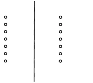
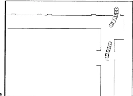
Shown in Figures 1 and 2 are two illustrative examples of using the modified

LMSE

classifier to separate two classes of patterns, where each class of pat- terns denotes a set of sampled points

of

a partial Corridor wall. Intuitively, the point patterns that are closer to the

ALV

location should be given larger weights. Therefore, the weights may be taken to be inversely proportional to the distances between the point patterns and the

ALV.

Figure 1 shows the result of applying the classifier to part of a straight corridor, and Figure 2 shows that of applying the classifier to a right-angle turning in a corridor. The portion of the decision boundary between the left and right walls in the vicinity of the

ALV

can be used to determine a collision-free local path for

ALV

navigation in the corridor. This indicates the feasibility of using the modified

LMSE

classifier for local path computation and collision avoidance in indoor environments. 2.2. Simulation Results

A

three-wheel, rectangular-shaped

ALV

is considered in the simulation, where the front wheel has driving power and the two rear wheels are free. A criterion for adjusting the front wheel direction is required so as to keep the

ALV

free from collision with the walls. Once the local navigation path (i.e., the portion of the decision boundary between the left and right walls in the vicinity of the

ALV)

is determined, the

ALV

will first turn and then move toward the path if the

ALV

is not right on the path.

A

table look-up control strategy

0 0 0 0 0 0 0 0 0 0 0 0 0 0

Figure 1. Use of the modified LMSE classifier to find a decision boundary between the left and the right walls in a corridor.

682

Journal of Robotic Systems-1 991

0 0 0 0 0 0 0

0 0 0 0

Figure 2.

pair of right-angle-turn walls in a corridor.

Use of the modified LMSE classifier to find a decision boundary between a

derived in ref. 21 is employed to obtain the front wheel direction of the ALV after the local navigation path is computed in each navigation cycle.

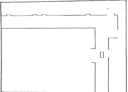
Figure 3 shows the top view of the walls of a corridor, including a right-angle turning. The rectangle in the figure denotes an ALV that travels along the corridor with a constant speed. The corridor wall model is stored in advance in

the ALV. In addition, a global path is needed for the ALV to travel in the corridor. Otherwise, it will not be able to decide whether to turn left or right when a turning corner is faced. Attached to each line segment (corresponding to the top view of a wall) in the model is a flag to indicate whether the ALV should be on the left or right side of the line segment while the ALV is traveling along the part of the corridor represented by the line segment. Together, these flags indicate a global path for the ALV in the corridor.

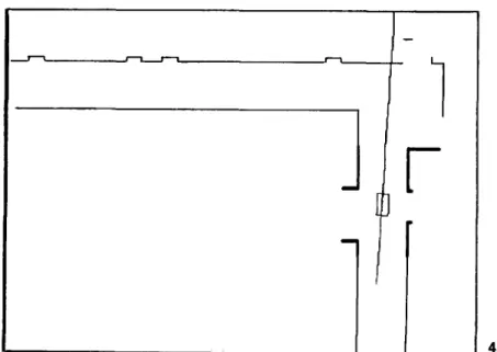
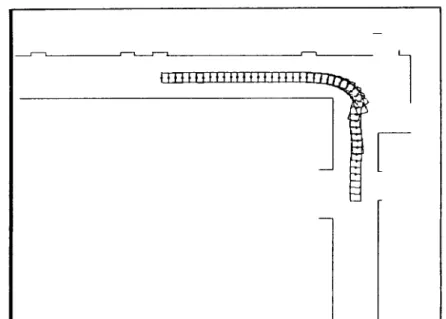
In each navigation cycle, the left and right walls in the vicinity of the ALV are imaged, extracted, and sampled as two classes of point patterns. The point patterns that are closer to the current ALV location are given larger weights (in proportion to the inverse of the point distance to the ALV location). And the computed decision boundary is used as the local navigation path of the ALV. Figure 4 shows simulated snapshots of the ALV at four different positions in the corridor, where the boldfaced line segments representing the wall portions around the ALV are used to determine the local navigation path. The continu- ous navigation trajectory of the ALV in the corridor is shown in Figure 5. The trajectory is seen to be well away from the walls. On an average, the computa- tion time for determining the local navigation path in each navigation cycle is about 0.2 s, using a PC/AT computer with an 80386-33 CPU.

3. ALV NAVIGATION AMONG MOVING OR STATIC OBSTACLES

In a real situation, when the ALV travels in the corridor, there may appear some unknown moving obstacles, e.g., human beings, which may collide with the ALV. To handle such a situation, the trajectories of the moving obstacles must be predicted first, and a safe local navigation path of the ALV is then computed according to the predicted trajectories of the obstacles and the envi- ronment of the corridor. It is desired that the prediction process be as accurate as possible without expensive computation. Linear prediction models usually given simple but effective solutions, especially for local collision-free path computation. The real-time LMSE estimation a l g ~ r i t h m ' ~ is thus employed in this study to approximate and predict the trajectories of moving obstacles. The modified LMSE classifier is then used again to determine the local navigation path of the ALV.

3.1. A Review on the Real-Time LMSE Estimation Algorithm Let x be a variable related linearly to a time variable t , that is, let

x = a t + b (1)

where a and b are two unknown constant parameters to be estimated by a sequence of m observations xi on x at m different time instants ti, i = 1, 2,

. . .

,

m. The m observation data provide the following set of m linear equations:

Journal of Robotic Systems-1 991

4a

4b

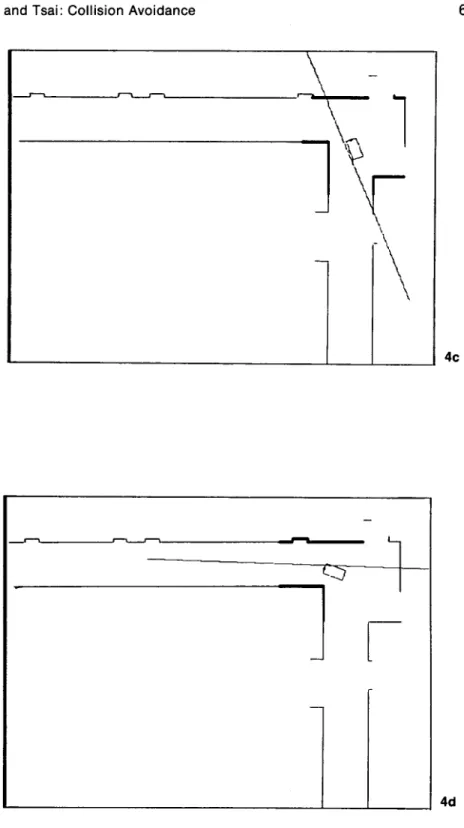
Figure 4. Simulated snapshots of an A L V at four different positions in the corridor of Figure 3. (a) An A L V is running along a straight corridor. (b) The A L V is approaching a right-angle turning in the corridor. (c) The A L V is turning left in the corridor. (d) The A L V has turned left in the corridor.

I

4c

4d

686

Journal of Robotic Systems-1991

I

r

H

1

Figure 5. The continuous trajectory of the ALV navigation shown in Figure 4.

which can be arranged into a simple form

X , = T,A, where

x,

=

Define an error vector Em = (el, e 2 ,

.

.

.

, em)t for each inexact solution A ,

such that

Let the optimal solution,

A m ,

be defined as the one such that the criterion function Jm

m

J, =

C

e?

i= I

is minimized.

A,

can be solved19 to be

When fresh experimental data are continuously supplied, it is desired to improve the parameter estimates by making use of the new information. If a recursive formula can be obtained, the estimates can be updated step by step without repeatedly computing the solution of eq. (2). For this, first define matrix P, as

Pm = ( T k T , ) - l .

Then it can be provenI9 that the solution Am+, for the (rn

+

1)th time instant can be computed from that of the rnth time instant, A m , as follows;

Am+, = Am

+

Yrn+lPrntrn+l{Xrn+l-t;+lam),

where

The real-time LMSE estimation algorithm is a simple modification of the above least-squares estimation algorithm in which an exponential weighting scheme is used to place heavier emphasis on more recent data. Such a type of data emphasis is appropriate for the locality property of collision-free path planning studied in this research. In the algorithm, the error function is defined as

in which the squared errors coming from more recent data are given larger weights than those from earlier ones. The smaller the A value, the heavier the

688 Journal of Robotic Systems-1 991

weights assigned to more recent data. P , is defined as

where

To apply the above real-time LMSE estimation algorithm to local obstacle trajectory prediction, assume that a sequence of m observations on the position of an obstacle have been made at m different time instants. By the following two sets of linear equations

xi = ari

+

b

yi = cri

+

d

i

= 1, 2,

. .

.

, m

i = 1, 2,

. .

.

, m

(4)

where (xi, yi) denote coordinates of the position of the obstacle at time instant t i , we can use the formulas in eq. (3) to estimate and update parameters a , b , c ,

and d using the fresh observation on the position of the obstacle obtained in each navigation cycle. Then we can predict the positions of the obstacle in the next cycles using these estimated parameters and the equations in (4).

3.2. Use of the Modified LMSE Classification Scheme for ALV Navigation Among Moving Obstacles

The modified LMSE classifier can also be used to plan a local collision-free path for an ALV in a corridor or in a planar workspace populated with obsta- cles. Again, the left and right corridor walls around the ALV are imaged, extracted, and sampled as two classes of patterns. For a moving obstacle, its current position and three-step-ahead predicted positions are regarded as a third class of patterns. The decision boundary between the left corridor wall and the obstacle and that between the right corridor wall and the obstacle are found by the modified LMSE classifier. For each decision boundary, the turn-

ing direction of the

ALV

is computed by the table look-up control strategy found in ref. 21. The decision boundary that results in the smallest turning angle for the

A L V

to adjust is selected as the local navigation path in the next navigation cycle so that the

A L V

will deviate as little as possible from its current location, while still being able to avoid collision with the obstacles.

3.3. Determination of ALV Speed

Once the local navigation path is determined, the turning direction of the

A L V

is computed by the table look-up control strategy found in ref. 21. If we can dynamically vary the speed of the

ALV,

the probability of collision will decrease. In the following, the maneuvering board technique used in nautical navigation16 is employed to determine the speed of the

ALV.

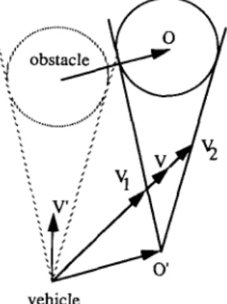
The basic maneuvering board technique is illustrated in Figures 6 and 7 , in

which obstacles are represented as enlarged circles such that the

ALV

can be represented as a point. Figure 6 shows the avoidance cone for a static obstacle, which is defined by two tangent lines from the

A L V

to the circle representing the obstacle. The movement direction of the

ALV

from one position to the next and its speed value form a velocity vector.

A

velocity vector is represented as

Figure 7. The avoidance cone for a moving obstacle.

690

Journal of Robotic Systems--1991

an arrow in Figures 6 and 7. A vector is said to fall within an area if the vector head is located in the area. Clearly, any velocity vector V that falls within the avoidance cone will result in a collision of the ALV with the obstacle.

The avoidance cone for a moving obstacle is shown in Figure 7 (consisting of the solid lines). Any velocity vector V of the ALV falling within this cone represents a collision course with the moving obstacle. The reason is that any such velocity vector V is the vector sum of a velocity vector V ' , which repre- sents a collision vector if the obstacle were static, and another velocity vector O r , which is the velocity vector 0 of the obstacle translated to the ALV loca- tion. That is, if the ALV runs with the direction of the vector V and at a speed between JVIJ and JV,J, as shown in Figure 7, the ALV will collide with the obstacle. Here, the lVll and IV2J values are called the boundary speeds.

For the ALV, we set a default speed value. In each navigation cycle, after the turning direction of the ALV is determined and the corresponding boundary speeds are computed, we can check if the default speed lies between the two boundary speeds. If not, the default speed is used as the ALV speed in the next navigation cycle. Otherwise, the boundary speed, which is closer to the current ALV speed, is used.

3.4. Static Obstacle Avoidance

The previous scheme proposed for moving obstacle avoidance can also be applied to static obstacles. In this case, just regard the predicted positions of a static obstacle to be all the same as the current object position, and consider the current object position as a single-pattern class. In fact, it is not necessary to distinguish static obstacles from moving ones in the proposed collision-avoid- ance scheme.

3.5. Simulation Results of Moving or Static Obstacle Avoidance

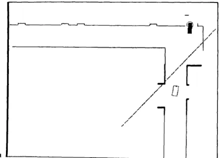
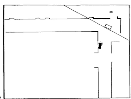
An example illustrating how an ALV avoids collision with an unknown mov- ing obstacle in a corridor is first given. Shown in Figure 8 are several simulated snapshots of an ALV and a moving obstacle at different positions, where the unfilled rectangle represents the ALV, the four small black rectangles denote the current position and the predicted obstacle positions of three steps ahead, and the circle denotes the current position of the obstacle. Figure 9 gives the top views of the continuous motions of the ALV and the obstacle at four time instants, illustrating the computed collision-free trajectory of the ALV. Shown in Figures 10 and 1 1 are two examples illustrating how an ALV avoids a static obstacle in a corridor. On average, the computation time for determining the local navigation path in each cycle is about 0.4 s in the case of avoiding a moving obstacle.

4. CONCLUSION

Several techniques have been integrated in this study to provide a collision avoidance scheme for ALV navigation. The real-time LMSE estimation algo-

8a

8b

Figure 8. Simulated snapshots of an ALV and a moving obstacle at six different positions. (a) An ALV and an obstacle encounter in the corridor. (b) The ALV is approaching the obstacle. (c) The ALV has avoided the obstacle. (d) The ALV is going to turn left. (e) The ALV is turning left. (f) The ALV has turned left.

692 _{Journal of Robotic Systems--1991}

8c

8d

8e

8f

I \

I

694

9a

9b

Journal of Robotic Systems-

U

991

Figure 9. Continuous trajectories of the ALV navigation and the obstacle movement of Figure 8. (a) In the first 6 navigation cycles. (b) In the first 11 navigation cycles. (c) In the first 13 navigation cycles. (d) In the first 29 navigation cycles.

9c

9d

t

696 Journal of Robotic Systerns-1991

Figure 10. Continuous trajectory of an ALV having avoided a static obstacle (case 1).

rithm has been employed to predict the motions of obstacles. A modified ver- sion of the LMSE classifier used in pattern recognition has been employed to plan a collision-free local path among obstacles. The maneuvering board tech- nique, used for nautical navigation, has been used to determine the speed of the ALV. In addition, a realistic control strategy on the translation and rotation of

a three-wheel ALV has been considered in the simulation. Combination of these techniques provides a feasible collision-avoidance scheme for guiding an ALV in a corridor to avoid unknown moving or static obstacles, as shown by the simulation results.

Further research may be directed to practically implementing the proposed approach on an experimental autonomous vehicle. Some urgent responses of the vehicle must also be considered when the computed collision-free path is too narrow for the vehicle to pass or when the vehicle is too close to the obstacle.

This work was supported by the Nationai Science Council, Republic of China under Grant NSC79-0404-EO09- 18. References 1. 2. 3. 4. 5. 6. 7. 8. 9. 10. 11. 12. 13. 14. 15. 16. 17.

H. P. Moravec, “The Stanford cart and the CMU rover,” Proc. IEEE, 71(7), (1983).

R. L. Madarasz, L. C. Heiny, R. F. Cromp, and N. M. Mazur, “The design of an autonomous vehicle for the disabled,” IEEE J . Robotics Automat., 2(3), (1986). A. M. Waxman, “A visual navigation system for autonomous land vehicle,” IEEE J . Robotics Automat., 3(2), (1987).

C. Thorpe, M. H. Hebert, T. Kanade, and S. A. Shafer, “Vision and navigation for the Carnegie-Mellon NAVLAB ,” IEEE Trans. Pattern Analysis Machine In-

tell., lO(3) (1988).

0 . Takahashi and R. J. Schilling, “Motion planning in a plane using generalized Voronoi diagrams,” IEEE Trans. Robotics Automat. 5(2), (1989).

R. C. Arkin, “Navigational path planning for a vision-based mobile robot,” Ro- botica, 7, (1989).

G. T. Wilfong, “Motion planning for an autonomous vehicle,” in Proc. IEEE Int. Conf. Robotics Automat., Philadelphia, PA, 1988.

S. Kambhampati and L. S. Davis, “Multiresolution path planning for mobile ro- bots,” IEEE J . Robotics Automat., 2(3), (1986).

D. T. Kuan, J. C. Zamiska, and R. A. Brooks, “Natural decomposition of free space for path planning,” in Proc. IEEE I n t . Conf. Robotics Automat., St. Louis, MO, 1985.

R. A. Brooks, “Solving the find-path problem by good representation of free space,” IEEE Trans. Syst., Man, Cybernet., 13(3), (1983).

R. C. Arkin, “Motor schema-based mobile robot navigation,” Int. J . Robotics Res., 8(4), (1989).

J. Borenstein and Y. Koren, “Real-time obstacle avoidance for fast mobile ro- bots,” IEEE Trans. Syst., Man, Cybernet., 19(5), (1989).

A. C. -C. Meng, “Free space modeling and geometric motion planning under unexpected obstacles,” in Proc. IEEE Int. Conf. ArtiJic. Intell. Applicat., San Diego, CA, March 1988.

K. Kant and S. W. Zucker, “Toward efficient trajectory planning: The path- velocity decomposition,” I n t . J . Robotics Automat., 5(3), (1986).

K. Fujimura and H. Samet, “A hierarchical strategy for path planning among moving obstacles,” IEEE Trans. Robotics Automat. 5( I ) , (1989).

L. Tychonievich, et al., “A maneuvering-board approach to path planning with moving obstacles,” in Proc. 11th Int. Joint Conf. ArtiJic. Intell., Detroit, MI, 1989. N. Kehtarnavaz and S. Li, “A collision-free navigation scheme in the presence of moving obstacles,” in Proc. IEEE Int. Conf. Computer Vision and Pattern Re- cog., Ann Arbor, MI, 1988.

698

Journal of Robotic Systems-I 991

18. J. P. H. Steele and G. P. Starr, “Mobile robot path planning in dynamic environ- ments,” in Proc. IEEE Int. Conf. Systems, Man, Cybernet., Beijing and Shen-

yang, China, 1988.

19. T. C. Hsia, System IdentiJkation: Least-squares Methods, Lexington Books, Lex- ington, MA, 1977.

20. P. A. Devijver and J. K . Kittler, Pattern Recognition: A Statistical Approach, Prentice-Hall, Englewood Cliffs, NJ, 1982.

21. P. Y . Ku and W. H. Tsai, “Model-based guidance of autonomous land vehicles for indoor navigation,” in Proc. of 1989 Workshop on Computer Vision, Graphics and Image Processing, Taipei, Taiwan, ROC, 1989.