應用全捲積網路所達成之弱監督音樂音訊及視訊事件偵測

(1)

國立臺灣大學電機資訊學院電機工程學研究所博士論文

Graduate Institute of Electrical Engineering

College of Electrical Engineering and Computer Science

National Taiwan University Doctoral dissertation

應用全捲積網路所達成之弱監督音樂音訊及視訊事件偵測 Weakly-supervised Event Detection for Music Audios and Videos

Using Fully-convolutional Networks

劉任瑜 Jen-Yu Liu

指導教授：鄭士康教授、楊奕軒博士

Advisor: Prof. Shyh-Kang Jeng and Dr. Yi-Hsuan Yang

中華民國 107 年 6 月

June, 2018

(2)

(3)

謝

本論文得以完成，首先要感謝兩位指導老師，鄭士康老師與楊奕軒老師。這幾年來你們在專業、做研究的方法與態度上、以及研究結果的呈現上，都給我相當大的指導與幫忙。也要謝謝你們很寬容的接受我對一些問題的看法與研究方法上的固執。謝謝口試委員鄭士康教授、楊奕軒博士、張智星教授、李宏毅教授、蘇黎博士以及深山覺博士撥冗參加我的論文口試，並給予我相當寶貴的建議。這些建議使本論文更加完備，也啟發我對未來研究的一些想法。

有我的家人與朋友在心靈上不間斷的支持，這篇論文才有可能完成。爸爸、媽媽、姐姐、嘉嘉和大腸在我人生的各個階段一直都是我最重要的支柱，尤其在就讀博士班期間更是如此。作研究、投稿和寫論文總會有低潮，有你們的陪伴讓這些苦悶的時刻輕鬆不少，也讓我有繼續堅持下去的動力。沒有你們這篇論文絕對是無法如此順利的完成，謝謝你們！

(4)

中文要

隨著視訊與音訊串流服務的流行，音樂音訊與視訊是現今最受歡迎的娛樂來源之一。音樂與音樂演奏包含相當豐富的資訊。為了能自動分析這些音訊及視訊以進一步進行檢索或教學，我們會想要使用機器學習來幫助偵測各式音訊及視覺事件。然而，機器學習的方法通常需要相當數量的訓練資料。在音訊及視訊中，標示這些訓練資料並不容易，因為手動標示的過程非常花時間而且乏味。在本論文中，我們探討如何以弱監督的方式，僅使用長片斷層級的標示來訓練偵測模型。

我們使用全捲積網路來達到音樂音訊與視訊之事件偵測。首先，使用全捲積網路在時間上偵測音樂音訊事件，如曲風、樂器、情緒等，並且使用樂器演奏資料庫來評估模型的表現。接著，我們將發展一個弱監督的架構來實現視訊中的樂器演奏動作偵測。此學習架構包含兩個輔助模型：聲音偵測模型與物體偵測模型。這兩個輔助模型也只使用長片斷層級的標記來訓練。它們將為動作偵測模型提供監督資訊。我們使用 5400 個經過手動標記的影像畫面來評估此訓練架構的表現。提出之訓練架構在時間與空間上相當大程度地改進了模型表現。

關鍵字：音樂事件偵測、樂器演奏動作偵測、弱監督學習、音樂自動標籤

(5)

Abstract

With the growing of audio and video streaming services, music audios and videos are among the most popular sources for entertainment in recent days. There are rich information in music and music playing. In order to automatically analyze these audios and videos for further retrieval or peda- gogical purpose, we may want to use machine learning to help with detecting audio and visual events. However, learning-based methods usually require a large amount of training data. In audios and videos, annotating these data are not easy because the process is time-consuming and tedious. In this work, we will see how to train such detection models with only clip-level annotations with weakly-supervised learning. We will use fully-convolutional networks (FCNs) for event detection in music audios and videos. First, we will develop FCNs for temporally detecting music audio events such as genres, instruments, and moods, which will be evaluated on an instrument dataset. Second, we will develop a weakly-supervised framework for detecting instrument- playing actions in videos. The learning framework involves two auxiliary models, a sound model and an object model, which are trained using clip-level annotations only. They will provide supervisions temporally and spatially for the action model. In total 5,400 annotated frames will be used to evaluate the performance of the proposed framework. The proposed framework largely improves the performance temporally and spatially.

Key words: music event detection, instrument-playing action detection, weakly-supervised learning, music auto-tagging

(6)

List of Figures

1.1 Example . . . 6

1.2 Example . . . 8

2.1 Desired output of event detection in audios and videos . . . 16

2.2 Supervised learning VS. weakly-supervised learning . . . 19

3.1 Expected effect of the accumulation layer. . . 23

3.2 The proposed FCN architecture. Given a trained network for clip-level prediction (the blue one), we replace the final pooling layer by an up- sampling layer for frame-level prediction (the red component). . . 25

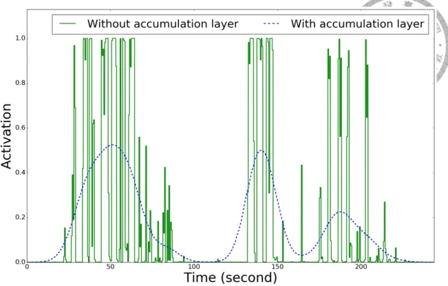
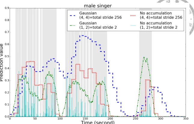
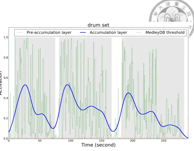
3.3 Smoothing effect of accumulation layers for a music piece from Med- lyDB. The frame-level predictions of four models with final max-pooling are shown. The micro F1 scores achieved by the four settings (Gaussian, stride 2), (Gaussian, stride 256), (No accumulation, stride 2) and (No accumulation, stride 256) are 0.658, 0.601, 0.158, and 0.601, respectively. This is the music piece entitled AlexanderRoss_GoodbyeBolero in the MedlyDB dataset. . . 34

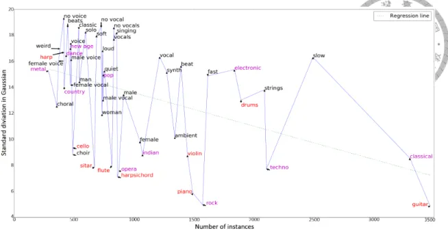
3.4 The standard deviation σ in Gaussian filter. x-axis is the number of in- stances in the training data, and y-axis is the quantity of σ of the classes after training. Instrument tags are in red color, and genre tags are in pur- ple. The green dashed line is the linear regression line of the points on the image. . . 36

(10)

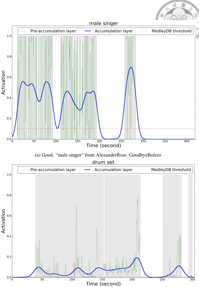
3.5 Visualization of frame-level predictions on MedleyDB test data: Good examples. . . 45 3.6 Visualization of frame-level predictions on MedleyDB test data: Bad ex-

amples . . . 46 3.7 Visualization of frame-level predictions on MagnaTagATune test data. They

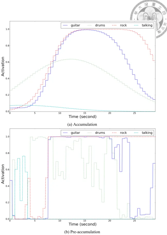
show predictions of four tags annotated on the clip. The outputs from accumulation layer and from pre-accumulation layer are shown. Both of them are from the same model. Title: jackalopes-jacksploitation-04- kentucky_applejack-0-29. . . 47 3.8 Visualized frame-level results. Red line is the ground-truth, and blue de-

notes frame-level prediction. . . 48 4.1 Four levels of supervisions: Video tag as target (VT) and Object as target

(OT) (continued in Figure 4.2). g is the instrument index, t is the temporal index, and (i, j) is the spatial coordinate in the output map. [V_g] is the vector of the video tags, [ ˆO^u_g,t,i,j] is the binarized output of the object model, [ ˆS_g,t^v ] is the binarized output of the sound model, and [A_g,t,i,j] is the output of the action model. Darker shade represents higher activation where activation values are between 0 and 1. Each cuboid in the figure represents an output tensor produced by a model at a given time t, and the three axes of a cuboid represent the instrument index g and the spatial coordinate (i, j), respectively. The t above or below a cuboid represents its temporal index. 51

(11)

4.2 Four levels of supervisions: Sound as target (ST) and Sound×Object as target (SOT). g is the instrument index, t is the temporal index, and (i, j) is the spatial coordinate in the output map. [V_g] is the vector of the video tags, [ ˆO_g,t,i,j^u ] is the binarized output of the object model, [ ˆS_g,t^v ] is the bi- narized output of the sound model, and [Ag,t,i,j] is the output of the action model. Darker shade represents higher activation where activation values are between 0 and 1. Each cuboid in the figure represents an output tensor produced by a model at a given time t, and the three axes of a cuboid repre- sent the instrument index g and the spatial coordinate (i, j), respectively.

The t above or below a cuboid represents its temporal index. . . . 52 4.3 Architecture of the action and object models. Details of the model archi-

tecture are described in TABLE 4.2. . . 56 4.4 Examples of the manually annotated key points (red dots) of instrument-

playing actions. I annotate the locations that are most directly responsible to making the instrument sounds as described in Section 4.2.3. Best seen in color. . . 65 4.5 Effect of different temporal resolutions of dense optical flows. The blue

solid line and the red dashed line are the validation losses and the test temporal AUC, respectively, of the action models trained with different resolutions of dense optical flows. The validation loss (the lower the better) and the test AUC (the higher the better) are both optimal at the resolution of 7.8 frame-per-second. . . 71 4.6 The result of instrument-playing action detection as a function of different

training targets. As the level of supervision changes from left to right, the result of action detection becomes cleaner and more accurate. The origi- nal videos of the two examples are uploaded by Jeremy Cohen (YouTue ID: 2G2VaBX24So) and Krishan Chotoe (YouTube ID: 55_RhFOyRgk), respectively, both of which are under Creative Common license. . . 76

(12)

4.7 Examples of predictions of all nine instruments from the action model

SOT0503 . . . 78

4.8 Prediction of the weakly-supervised object model used in this paper and the prediction of a Faster R-CNN model. The red rectangle frames are the predictions of the Faster R-CNN model, and the blue shades are the predictions of the weakly-supervised object model. Best seen in color. . . 81

4.9 Procedure of deriving stacked average movements. . . 84

4.10 Stacked average movements derived from 96 filters of Conv1 (action model SOT0503). . . 85

4.11 Procedure of deriving the characterizing stacked average movements for the instruments. . . 86

4.12 Characterizing stacked average movements of the 9 instruments. . . 87

A.1 A GUI for demonstrating the proposed model . . . 91

A.2 A song with female and male vocals¹ . . . 91

A.3 Confusion between high-pitched male voices and female voices² . . . 92

A.4 Confusion between guitar and piano³ . . . 93

A.5 Confusion between guitar and male voices⁴ . . . 93

A.6 Confusion between violin and cello⁵ . . . 94

(13)

List of Tables

3.1 Best performance for the clip level and frame level. The baseline in frame- level performance is derived by simply predicting all frames as positive (i.e. all ones). . . 30 3.2 Effect of thresholds for frame-level predictions. Thresholds are derived

either from MedleyDB or MagnaTagATune. “Early conv.” refers to the number of layers in early convolutions. . . 31 3.3 Accumulation layers. The models either use no accumulation, use accu-

mulation with Gaussian of fixed standard deviations (σs), or use accumu- lation with Gaussian of adaptive standard deviations (σs). 50 classes for clip-level and 9 classes for frame-level . . . 33 3.4 Effect of multi-scale inputs. Inputs of 1 scale, 3 scales, or 6 scales are

experimented. . . 33 3.5 Effect of different total stride sizes. The total stride is related the resolution

of the CNN. The larger the total stride, the worse the output resolution. We control the total stride by controlling the number of early convolutional layers. The stride size is 4 for every early convolution layer. . . 35 3.6 The performance of models trained directly with frame-level annotations.

The number under “late layers” represents the number of units used in a layer. If two numbers are present, there are two layers. . . 37

(14)

3.7 This table provides the number of data in each dataset, the learned standard deviations σ of Gaussian filter layer after training, and the performance of our model. The US dataset evaluated with AUC score represents the performance of frame-level predictions, and the accuracy tested on US8K is the clip-level evaluation result. . . 41 3.8 The comparison between the clip-level accuracy of basic setting and of

adding one of multiple scales, data augmentation, and Gaussian filter to the model. . . 42 4.1 Architecture of the sound model. It is an FCN adapted from the model

proposed by the authors in their previous work [1]. There are three scales of input feature maps, and each of them has their own stack of early convolutions (Conv1 and Conv2). ‘RF’ represents receptive field and ‘St’

represents stride size. . . 54 4.2 Architecture of the action model and the object model. It is an FCN

adapted from the CNN model VGG_CNN_M_2048 used in [2]. ‘RF’ represents receptive field and ‘St’ represents stride size, and ‘LRN’ represents local response normalization . . . 55 4.3 Datasets used in this paper and their data types, annotation types, and us-

ages. YT8M-IPA represents the proposed YouTube-8M-Instrument-Playing- Action dataset. . . 62 4.4 Models used in this paper and their input features, prediction types, and

training targets. . . 62 4.5 Properties of the nine instruments. The lower part of the table contains

the number of data in the datasets. In YT8M-IPA, the playing actions are annotated at the intersections of the action regions and the playing tools as described in Section 4.2.3. ‘frs’ represents frames. ‘imgs’ represents images. . . 64

(15)

4.6 Evaluation of the sound models for instrument sound detection. The sound model trained with AudioSet outperforms the one trained with YouTube- 8M and the one (the model in our previous work [1]) trained with the music dataset MagnaTagATune. We use ‘Acc.’ as shorthand for Accordion. 66 4.7 Evaluation of the object models for instrument object detection. They are

tested on the instrument images with bounding boxes collected from Ima-

geNet (HIT RATE). The one initialized with a pre-trained model VGG_CNN_M_2048 (With pre-training) outperforms the one with random initialization (From

scratch) by a large margin. . . 69 4.8 Evaluation of the action models for instrument-playing action detection.

The ST and SOT models outperform other models temporally because they have temporal supervisions from the sound model, while the OT and SOT models outperform other models spatially because they have spatial supervisions from the object model. . . 73 4.9 Instrument-wise action detection performance (Temporal in AUC). The

best temporal scores are all achieved by ST and SOT that have temporal supervisions from the sound model. . . 74 4.10 Instrument-wise action detection performance (Spatial in pixel). The best

spatial scores are mostly achieved by OT and SOT that have spatial supervisions from the object model. . . 74 4.11 Temporal performance of the ST action models by using as the training

target either the sound model trained with the video dataset AudioSet (AS) or the one trained with the music audio dataset MagnaTagATune (MTT).

The ST action model using the AudioSet sound model outperforms the one using the MagnaTagATune sound model in all instruments. . . 76 4.12 Fusion of different streams of modalities after training (Temporal perfor-

mance in AUC). The output of an action model is fused with the output of the sound model and/or the output of the object model by point-wise multiplication. The fusion significantly improves the result. . . 79

(16)

4.13 Fusion of different streams of modalities after training (Spatial performance in Pixel). The output of an action model is fused with the output of the sound model and/or the output of the object model by point-wise multiplication. The fusion significantly improves the result. . . 80 4.14 The performance of the action models trained with a Faster R-CNN ob-

ject model in comparison with the action models trained with a weakly- supervised object model. We train the action models with five thresholds in the object model: 0.1, 0.3, 0.5, 0.7, and 0.9. We let them use their own best threshold for each instrument because they are quite different models so they may have different optimal thresholds. We use 0.5 as the threshold in the sound model for SOT models. . . 83

(17)

Chapter 1 Introduction

Music-related audios and videos are among the most popular sources for entertainment. There are rich information in music and music playing. The audio parts are with instrument sounds, vocal sounds, or the pattern of blues, rocks, jazz, etc. Many other properties like tempos, and pitches are often recognized. In a performance recorded in video, we can expect to see instrument-playing actions, the sounds made by the instruments, the expression of the players, the interaction of the players with audience, and so on. Objects such as humans and instruments, as well as actions such as dancing and instrument playing are often included in the scene. All these properties can be considered as events, because they occur in some places during a period of time and are with varying time durations.

In order to analyze these audios and videos automatically, it is important to detect these events.

Machine learning provides ways to automatically label these audios and videos. How- ever, learning-based methods also require an amount of data for training the models. Man- ually labeling the temporal and spatial locations of these events is often tedious and time- consuming.

Let’s see what we need to do for annotating a music piece with instrument labels. A difference between annotating an image and annotating a music piece is that we have to take time to listen to the music from the beginning to the end. We cannot skip the middle parts because there might be important information there. As we are listening to the music, we start to annotate the music with instrument labels. However, there are often multiple

(18)

instruments playing at the same time and some instruments sound similar, so listening once is often not enough. We have to listen to the same music several times. This is just for one song, and it is very tedious. Imagine how many works we have to do if we want to annotate the instrument objects and instrument-playing actions videos.

Thus the main topic of this dissertation is about how to alleviate the difficulty of labeling annotations by utilizing weakly-supervised learning is the main topic of this work.

We will investigate how to use clip-level annotations to train a model that can detect music audio events and instrument-playing actions. In contrast to the difficulty of collecting data annotated with detailed temporal and spatial information, audio and video data with simple clip-level annotations are much easier to acquire from websites such as YouTube and Last.fm as well as publicly available datasets such as YouTube8M and AudioSet.

In this work, methods are proposed to learn the temporal and spatial locations of audio events and actions in audios and videos. For the event detection in music audios, fully- convolutional networks (FCNs) are used as the base models for detection. Two mech- anisms are used to further enhance the performance. First, Gaussian filters are used to capture the temporal characteristics of different types of labels, which adapt its width to different labels in the training process. Second, multiple input feature maps with different FFT window sizes are used to capture information from different temporal scales.

Extending from the the method for weakly-supervised music audio event detection, we will see that the instrument-playing action detection can also be done in a weakly- supervised way. For videos, the annotations of actions are even more difficult to collect because they have to be labeled both temporally and spatially. We can observe that instrument playing is among a special type of actions which involves a tool (instruments) and the tool would make sounds (music sounds). This work proposes a way to utilize this property to automatically produce extra supervisions in learning from two auxiliary models.

(19)

1.1 Contributions

• A novel model is proposed for weakly-supervised audio event detection by using fully-convolutional networks

• A novel framework is proposed for weakly-supervised instrument-playing action detection by using two auxiliary networks to provide supervisory signals

• A new dataset is annotated and released for evaluating instrument-playing action detection

• Extensive experiments are conducted to evaluate the proposed models

• The codes are made publicly available for both music audios (https://github.

com/ciaua/clip2frame) and music videos (https://github.com/ciaua/

InstrumentPlayingDetection).

1.2 Event detection in music audios

The problem of event or object localization arises in many areas of information processing. In speech recognition, the temporal correspondence between the spoken and the recognized words is required [3–6]. In visual object recognition, people want to know not only whether an object (e.g., a cat) is present in an image, but also where the object really is within the image [7–11].

The localization problem also exists in music auto-tagging, whose goal is to automatically label a music clip with attributes such as instruments, genres/styles or acoustic prop- erties [12–15]. Although people tend to describe such attributes simply as tags, we can also view them as descriptors of music events. For example, an instrument tag “guitar”

can be thought of as “the presence of guitar.” A genre tag such as “Jazz” is usually used to describe a whole piece of music, but it can also be rephrased as “having a Jazz flavor”

which describes parts of the piece. From this point of view, a tag should be associated with starting points and ending points in a music piece, if the tag applies to multiple parts of the piece. Localizing the music events is beneficial for many tasks in music information

(20)

retrieval. For example, a user would not know that there are Jazz elements in parts of a music piece, if the piece is only globally labeled as being “Pop.” In music search, a user may look for short segments of music pieces featuring certain attributes, such as “metal screaming vocal,” “a saxophone solo” or “outside improvisation.” If several instruments are used in a music piece, localizing the instruments in time gives us a better understanding of the overall structure and organization of the piece.

Music event localization/detection, however, is seldom addressed in the literature, mainly due to the scarcity of labeled data. In speech recognition, localization is achieved by collecting frame-level annotation and training prediction models directly in the frame level [3, 4]. In visual object detection, manual annotation of the so-called bounding boxes around the objects of interest is usually needed for training a model for localization [7].

Although music event localization may sound similar to these two tasks, labeling music events by hand is arguably more difficult. For example, while speech data usually have only one active speaker at a time [16], it is typical to have multiple instruments, vocals, or styles in music, rendering it a multi-label problem [17]. As opposed to image, labeling music requires certain level of domain expertise. Localizing events in a time stream is also more labor-intensive and time-consuming. In consequence, it is not surprising that most datasets available for music auto-tagging contain only clip-level annotations [15, 17].

In light of these observations, a novel approach is proposed in this work that conquers the scarcity of labeled data for music event localization by using only clip-level annotation of tags in the training phase. In music event detection, the contribution of this work is threefold.

First, this work represents one of the first attempts that systematically investigate the localization problem in music auto-tagging. In addition to building a machine learning model that is able to make both clip-level and frame-level prediction of tag occurrence, a series of experiments are also presented to gain insights into issues specific to the frame- level prediction task, namely music event detection or localization. In general, “event detection” (or “event localization”) is about locating the start and end time of an event, whereas “frame-level tagging/prediction” is about predicting the labels at frame level. In

(21)

this work, event detection is achieved by frame-level prediction, and we will use them interchangeably because we can derive the other if we have one.

Second, by extending a convolutional neural network (CNN)-based approach to visual object recognition [10], a fully-convolutional network (FCN) model is developed for predicting and detecting music events in unseen music by training on only clip-level data.

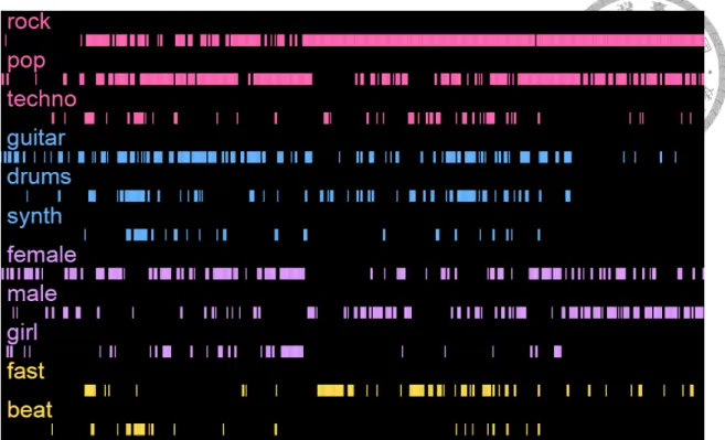
Our model is designed to account for the variable duration of music events and the tem- poral information of music. This is done by adding an accumulation layer that uses a Gaussian filter of tag-dependent length for assembling local information, and by feeding multi-scale audio features to the FCN. Different from existing CNN models for musical feature extraction [13, 14], our FCN model can deal with music of arbitrary length. An example of the detection result of the proposed model is shown in Figure 1.1. A song can have different types of properties such as genres, instruments, vocals, and tempos.

Furthermore, the properties may only appear at some parts of the song, so we can see in Figure 1.1 that the detection result of different tags do not coincide. The code and the trained model are available online¹.

Third, as no evaluation framework has been proposed for music event localization trained with clip-level annotations, this work is also motivated to propose such a framework to facilitate objective evaluation of the prediction result. In this work, we will see that existing multi-track music datasets originally intended for studying musical source separa- tion or transcription problems can be nicely used to evaluate frame-level prediction of instrument tags, and demonstrate such an evaluation by using the music auto-tagging dataset MagnaTagATune [17] and a recently proposed multi-track dataset called MedleyDB [18].

Visualization of some prediction results is also presented, which can be used to subjec- tively evaluate the performance for both instrument and non-instrument tags.

1.3 Instrument-playing action detection in music videos

With the popularity of social media and online sharing, people are sharing a large amount of videos online every day. These videos often contain human activities, so hu-

1https://github.com/ciaua/clip2frame

(22)

Figure 1.1: An example of the music event predictions.

man actions or movements are informative components in these videos. Therefore, automatically recognizing the types of the actions and locating the actions in videos can help understand and retrieve videos [19]. This task is often called “action detection” [19–26].

For fully-supervised learning approaches, detailed temporal and spatial annotations of actions are usually needed for action detection. However, these annotations are difficult to acquire because the labeling is labor-intensive and time-consuming [19]. In recent years, researchers have proposed various strategies to alleviate this issue [19, 21, 26].

An observation can be made that the objects and sounds in several types of videos might also be used to alleviate this issue. In a large amount of videos, both the objects and sounds signify the key points of the actions. Examples include videos with instrument playing [27], videos with violent content [28], and sport videos [29]. For example, when we hear a guitar solo and see a musician holding a guitar in a video, it is pretty likely that the guitar solo comes from the musician’s playing actions. The hitting actions in ball games often contain the acting objects, such as feet, hands, rackets, or bats, as well as the accompanied sounds of hitting. This relationship between actions, objects, and sounds provides an opportunity to infer the appearance of actions from objects and sounds.

(23)

Specifically, from the actions in the videos where sounds and objects signify the key points of actions, we can observe the following two common properties:

Action-in-object The spatial location of an action is close to (e.g. at the border or within) the spatial location of objects (e.g., instruments, bats, balls, or weapons).

Action-making-sound A specific type of actions is associated with a specific type of

sounds that the actions make.

Action-in-object together with the region of the objects in the scene may give us clues regarding where the actions occur spatially, while action-making-sound together with the temporal activation of the sounds in the video frames may help us temporally locate the actions. In contrast to annotated action data, annotated data of objects and annotated data of sounds are easier to acquire. Therefore, in this work, a method is proposed to train a sound model specifying when the actions occur and train an object model telling us where the objects are. These two auxiliary models act as teachers to inform the action model when and where to pay attention to. We feed only the motion information (dense optical flows in this work) to the action model, so it is forced to learn when and where the actions occur by only motions with the help from the two auxiliary models. An interesting feature of this proposed framework is that it does not need annotated data of actions at all in the training process. This proposed framework is considered as a weakly-supervised learning one, because the model is trained to predict when and where the playing actions are in videos by using only information regarding whether an instrument appears in a video clip in the training phase. The proposed framework is depicted in Fig. 4.2b (Figs. 4.1a, 4.1b, and 4.2a are variants of the proposed framework that will be discussed in Section 4.1.2).

We will focus on the instrument-playing actions in music-related videos in this work.

Music is one of the most popular types among online videos (ranked number two accord- ing to the study of Cheng et al. [30]), and instrument playing is among the most common scenes in these videos. For the audio aspect of instrument playing, automatic detection of instrument sounds has been widely studied in music information retrieval (MIR) [31–35].

It helps people understand the content of the music. However, the visual aspect of instrument playing remains largely unaddressed in literature. In addition to the sounds of instru-

(24)

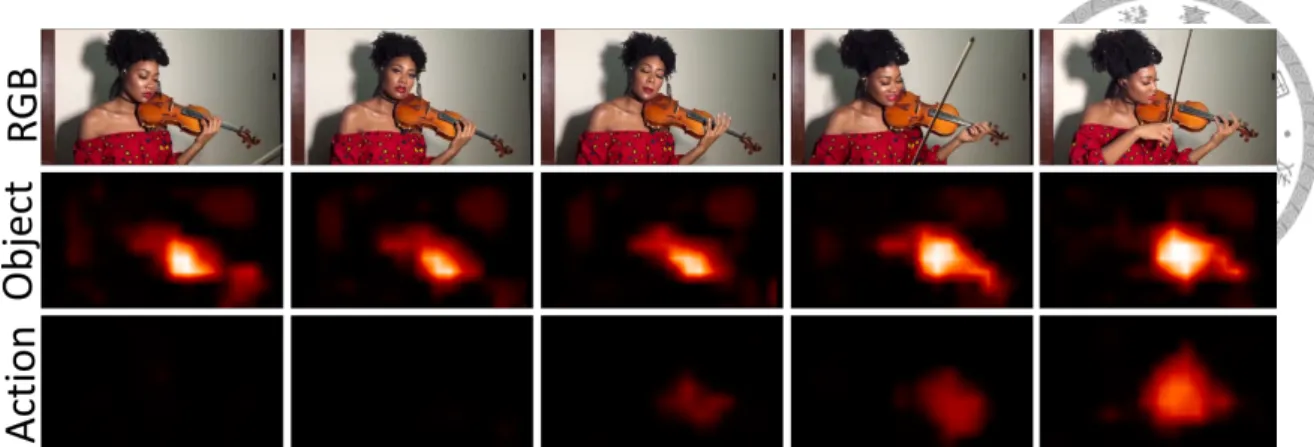
Figure 1.2: An example of the action predictions. They are five consecutive frames with one-second interval.³

ments, the visual appearances of instruments and instrument-playing actions also provide us important information about the music-related videos. In order to understand music- related videos, we need to know which instruments are played, when the instruments are played, and where the playing actions occur in the scene.² For example, in a video of a piano concert, the pianist may first walk into the scene, sit down, and then start to play the piano. In this case, the piano is not played until the pianist sits down and is ready.

We may want to know when the playing begins, the relative position of the piano to the scene, the relative positions of the hands to the piano, etc. There are also attempts to model the audio and visual information jointly for music information retrieval tasks [37,38]. For example, Schindler et al. investigated music genre classification by aggregating audio fea- tures and visual features together as the input features to a classifier [37]. This approach could improve the input feature of the model, but cannot circumvent the lack of annotated data.

In light of these observations, the goal of this work for music videos is to train a model to automatically pinpoint the instrument-playing actions temporally and spatially in videos with instrument-playing scenes without detailed annotations. In contrast to the abundance of annotated data available for either object recognition (including instruments), such as

2And even how the instruments are played—the gesture, the playing technique, the expression etc [36].

This is left as a topic of future research.

3The RGB snapshots are cropped from an YouTube video (ID: 3hjHJo452dY, uploaded by Zara and Nicola) with Creative Commons license.

(25)

ImageNet⁴ [39], or sound recognition, such as AudioSet⁵, we have no available dataset specifying the location of the playing actions in the scenes. Therefore, we can train the action model by utilizing the two properties mentioned above together with a trained sound model and a trained object model. We use the spatial locations of instrument objects and the temporal locations of the instrument sounds to help the detection of playing actions, but do not join the input features. In this way, we have a more flexible model that can work even if the audio is degraded due to factors such as environmental noises, audio track loss, or audio compression artifacts [40]. We human beings can guess if an instrument is played simply by the action, gesture, and the relative positions of hands or bows to instruments.

An example of action detection result is shown in Fig. 1.2. The violinist is not playing initially, and then she gradually raises the bow and starts playing in the final two frames. It shows that the the instruments and the playing actions do not always temporally coincide, and the action model should be able to handle this situation.

In order to investigate weakly-supervised instrument-playing action detection, three as- pects are contributed in this dissertation. First, a training framework is proposed to learn the temporal and spatial locations of the actions without detailed annotations by utilizing the object and the sound information. Furthermore, we can utilize the object and sound information to further improve the result after the action model is trained by a simple yet effective method of model fusion. Second, although the proposed method does not require detailed location information in training, for the purpose of evaluation, I manually annotated totally 5,400 frames from 135 videos with detailed locations of instrument-playing actions. Third, comprehensive experiments are conducted to investigate the effects of different components in the framework (Section 4.3). The action patterns the neural network learns for each instrument are analyzed.

4http://www.image-net.org/

5https://research.google.com/audioset/

(26)

1.4 Overview

This dissertation consists five chapters. In this chapter, Chapter 1, the task of event detection in audios and videos is introduced, including some general information and related work. Chapter 2 introduces the background knowledge used throughout this work, including the difference between supervised learning and weakly-supervised learning, the definition of event detection in the context of this work, and the basics of neural networks.

Then, the proposed method of conducting weakly-supervised music event detection is detailed in Chapter 3. In Chapter 4, the weakly-supervised music event detection is used to help weakly-supervised instrument-playing action detection in videos. Finally, I conclude this work in Chapter 5.

(27)

Chapter 2 Background

In this chapter, we will first survey studies related to this work. Then, concepts used throughout this work will be introduced. The concepts include the definition of event detection, weakly-supervised learning, fully-convolutional networks, and the features used.

2.1 Literature survey

In this section, we will review and discuss the studies related to this work. They are divided into three categories: detection and classification in audios, detection and classification in videos and images, and weakly-supervised learning.

2.1.1 Detection and classification in audios

A considerable amount of work has been made for music auto-tagging, mostly fo- cusing on only clip-level prediction (i.e., whether a tag can be applied to a music piece) [12–15, 41–44]. Although audio features are usually extracted in the frame level, the objective of learning is to make clip-level prediction. In recent years, deep neural network architectures have been found superior to competing machine learning models for music auto-tagging [13, 14, 45]. For example, Dieleman et al. have shown the effectiveness of CNN in learning features for music auto-tagging [13]. However, this CNN model can neither deal with music of arbitrary length nor perform frame-level prediction.

(28)

Some studies investigate audio auto-tagging with finer granularity. Essid et al. apply hierarchical clustering for frame-level instrument recognition with temporal annotations of instrument occurrences [46]. Mandel et al. study the tag relationships inside a track and between tags with 10-second clips [47–49]. Frame-level prediction on music auto-tagging was discussed by Wang et al. [50]. Parascandolo et al. conducts polyphonic sound event detection with recurrent neural networks [51]. The main difference between the proposed method in this work and those in these studies is that the proposed method can predict at a temporal granularity finer than the granularity of the training data.

In recent years, the multimedia and MIR community starts to address the difficulty in collecting training data for frame-level predictions. Kumar et al. investigated the prob- lem of audio event detection with SVM and neural networks with weak-labeled data [52].

Schlüter utilized saliency maps to iteratively train a model that can recognize singing voices in the frame level [53]. In this work, we also utilize an FCN model to derive the frame-level instrument sound predictions. However, we will further use the frame-level instrument sound predictions as the training target for the visual action model, not only as the end product itself.

Instrument recognition has been an active research topic in MIR. Essid et al. extracted various audio features and applied hierarchical clustering and SVM for instrument recog- nition [31]. Han et al. proposed a CNN structure to recognize the predominant instrument in music [34]. Slizovskaia et al. used both audio and visual features as the input and applied CNNs for the task of instrument recognition [38]. The goal of these works is to recognize the instrument sounds with audio or audio-visual information as the input. In contrast, one of the goals in this work is to detect the instrument-playing actions at frame level by the visual cues in a video.

2.1.2 Detection and classification in videos and images

Zhou et al. identified the difficulty in acquiring action annotations for action detection and proposed a way to estimate the temporal and spatial extents of the actions [19]. They proposed a trajectory split-and-merge algorithm to first segment the background and the

(29)

foreground moving objects by using dense optical flows, and then they used the segmentation information to derive the temporal and spatial extents of the actions. Then, they used a latent SVM to classify these segmented patches and locate the actions. We share a similar goal to derive the temporal and spatial extents in our proposed framework, but we investigate utilizing two other modalities to estimate the extents, instead of using the dense optical flows.

Oquab et al. proposed to use fully-convolutional neural networks (FCNs) to realize weakly-supervised learning for images [10]. By replacing the fully-connected layers in conventional convolutional neural networks (CNNs) [54,55] with fully-convolutional layers, the model produces an output map that indicates the activation values at different locations. We use this method to do spatial weakly-supervised learning for both action detection and object detection in this work.

There have been several studies on weakly-supervised object detection or segmenta- tion. Hartmann et al. used support vector machine (SVM) [56] for weakly-supervised object segmentation in videos [57]. Liu et al. used a nearest neighbor-based method to perform weakly-supervised object segmentation in videos [58]. Prest et al. used motion cues to produce candidates of temporal tubes that locate a moving object and trained the object detector with a subset of the tubes [59].

Bojanowski [21] and Huang et al. [26] tackled the problem of weakly-supervised ac- tion detection. In their study, they only knew the sequence of actions and they had to align the actions with the frames in a video clip. They proposed different ways to align the action sequence. Our work is different from theirs in two ways. First, we use auxiliary sound and object models to learn to assign labels to video frames, instead of based on the sequence of labels assigned by human. Second, they only attempt to predict the labels temporally but not spatially.

Simonyan et al. proposed a two-stream framework for action detection by using an object stream and an action stream [22]. They experimented with fusing the two streams either by averaging the output scores of the two models or by using SVM to do the final classification. Feichtenhofer et al. extended Simonyan’s work by using different ways of

(30)

model fusion [25], and Ng et al. extended Simonyan’s work by incorporating information across longer period of time through temporal pooling and LSTM [23]. Our method also contains multiple streams. However, we use FCNs for all the three streams instead of the conventional CNNs because we want not only to classify the videos but also to locate the instruments, the actions, and the sounds. Furthermore, the models are fused only after they are separately trained.

The proposed method for action detection in this work is also related to supervision transfer introduced by Gupta et al. [60]. Given two learning tasks where task 1 has large annotated data while task 2 does not, Gupta et al. proposed to use the output of a middle layer in the well-trained network in task 1 to provide supervision to a middle layer of the network in task 2. In this way, the supervision is transferred. In this work, we also want to seek for more supervisions to the instrument-playing actions from two other modalities, but we provide the supervisions directly in the output layers by the physical relationships of the three modalities that are indicated by the two observations stated in Section 1.3.

The temporal and spatial supervisions are also exploited in addition to the instance-level label supervision in this work.

2.1.3 Weakly-supervised learning

In recent years, unsupervised learning, weakly-supervised, and semi-supervised learning have received lots of attentions in video processing [61–64]. This trend is partly due to the lack of supervisory signals in videos, but it is also because the multi-modal nature of videos and the temporal continuity of videos provide a good environment for learning feature representations by the dependencies between modalities or between frames without external supervisions. For example, Aytar et al. [61] and Arandjelović et al. [63]

proposed to match the audio and visual information to unsupervisedly learn features from a large amount of videos and use only a few labeled data for training a classifier based on the learned features. Aytar et al. [64] further included text in addition to the audio and visual information for feature learning. In contrast to the aforementioned multi-modal approaches, Canziani et al. [62] proposed a CortexNet framework to learn features by

(31)

matching neighboring frames in videos. Similar to these works, our proposed framework also represents an attempt to increase supervisory signals by utilizing multiple modalities of videos for a challenging action detection task.

Labeling the bounding boxes of objects in an image requires more labors than annotating the presence of objects does. Therefore, weakly-supervised approach for visual object localization with only image-level annotations has attracted increasing attentions in recent years [8–11]. Among the prior arts, our approach is closest to the model proposed by Oquab et al. [10], a multi-instance learning variant and also based on CNN. A key idea proposed in this work is to use the so-called full convolutions, so that the model can pro- cess images of arbitrary size. In this way, they can resize an input image arbitrarily in a multi-scale manner to locate a visual object. Being inspired by this approach, our model has two distinct features. First, we adopt a different way to achieve multi-scale learning for audios, as music cannot be easily “resized” as images. Second, we use a dedicated layer to deal with the temporal dimension in music, which is absent in images.

Visual event or action detection in videos, which also have a temporal dimension, has also been studied [22, 65, 66]. Similar to music event detection, this problem requires weakly-supervised learning because the annotation is at the video clip level. However, little work, if any, has been proposed to address localization problem for visual events in videos.

2.2 Event detection as a multi-label classification prob- lem

This work tackles the problems of event detection in both audios and videos. The detection in audios involves locating the events in time, while the detection in videos involves locating the events in space and time. Both of the two cases can be seen as multi- label classification problems.

First let’s consider the case of audios. In audio event detection, we want to label each temporal point with the properties we are interested. The desired output is in the form

(32)

(a) Audio (b) Video Figure 2.1: Desired output of event detection in audios and videos

A = [A₁, A₂, ..., A_T], where A_t = [a₁, a₂, ..., a_K]^T is a column vector of K elements, a_k∈ 0, 1, and K is the number of the labels in the entire dataset. An illustration is shown in Figure 2.1a. A can be seen as a K× T matrix.

In video event detection, we want to label each pixel at each temporal point with the properties we are interested. Therefore, the desired output is in the form V = [V₁, V₂, ..., V_T], where V_t= [v₁, v₂, ..., v_K] is a K×H ×W tensor, each vkis a H×W matrix representing the spatial information, K is the number of the labels in the entire dataset, and H and W are the height and width of the image frame. An illustration is shown in Figure 2.1a. V can be seen as a K× T × H × W tensor.

For the event detection in either audios or videos, there are no constraints on how many labels a spatial or temporal location can have, so they are multi-label classification problems [67].

A more common tasks than muti-label classification problems are multi-class classification problems. In a multi-class classification problem, it is assumed that there is only one correct answer at a given unit. For example, in image recognition, it is assumed that each image contains only one prominent object [55]. In semantic segmentation, it is also assumed that there is only one class at each pixel [68]. In genre classification in music, it is also often assumed that there is only one genre in one music piece [69].

In contrast, in multi-label classification problems, we could assign 0, 1, or more correct labels at a given unit. In music auto-tagging, a music piece can have multiple properties at the same time. For example, a Rock song can be labeled with ‘Rock,’ ‘Male,’ ‘Female,’

(33)

‘Happy,’ ‘Guitar,’ ‘Drum,’ and ‘Bass’ at the same time.

There are some implications due to this difference in practice. In the context of su- pervised learning, assume we have a vector x = [x₁, x₂, ..., x_n] which is the output of the final layer of a network at a given temporal/spatial location for n labels and a vector y = [y₁, y₂, ..., y_n] which is the corresponding annotation. In a multi-class classification problem, the nonlinear function applied to the output of the final layer of a network is usually a softmax function [55]:

Sof tmax(x_i) = exp(xi)

∑

jexp(x_j), (2.1)

and the corresponding loss function is a multi-class cross entropy:

∑

j

−yj· logxj (2.2)

.

In contrast, in a multi-label classification problem, the nonlinear function applied to the output of the final layer of a network is usually a sigmoid function [1]:

Sigmoid(xi) = 1

1 + exp(−xi), (2.3)

and the corresponding loss function is a binary cross entropy:

1 n

∑

j

−(yj · log(xj) + (1− yj)· log(1 − xj)) (2.4)

.

Furthermore, a threshold is needed in order to turn the real-valued network output into a yes/no binary output in a multi-label classification problem, while a threshold is not required in a multi-class classification problem.

(34)

2.3 Weakly-supervised learning

In contrast to the most common supervised learning in classification problems, weakly- supervised learning utilize data that have less or weaker annotations. Zhou recognizes different types of weakly-supervised learning [70], including incomplete supervision, inexact supervision, and inaccurate supervision. What these have in common is that they all have some sort of information loss in the supervisions.

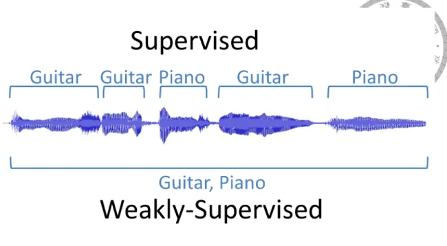
In incomplete supervisions, some data are labeled but some are not labeled. In inaccurate supervisions, the annotations may contain errors [70]. One major source of inaccurate supervisions is the web-crawled data [71]. In inexact supervisions, some supervisions are provided, but is not as exact as desired [70]. Inexact supervisions often appear in detection tasks such as semantic segmentation in images [72], action detection in videos [26], or sound event detection in audios [52]. These tasks are sometimes called multiple instance learning (MIL) [73]. For example, in an MIL situation, we are only told by the supervision that an image contains a dog, but we are not told where the dog and the dog could occupy only a small portion of the image. Supervisions are given, but they are not as exact as we desire.

In the existing works, ‘weakly-supervised learning’ usually refers to the inexact supervisions [1, 10, 74, 75]. This type of weakly-supervised learning is also what will be discussed in this work.

For either weakly-supervised learning or supervised learning, we may consider a dataset D = {(X1, y₁), (X₂, y₂), ..., (X_M, y_M)} [70], where Xi is an input sample and y_i is the corresponding annotation. Xi could represent different things in supervised learning and weakly-supervised learning.

Assume that we want to know whether a song contains guitar playing and where they are. In this case, X_iis a music audio signal or feature of the shape K× T , where K is the dimension of the feature and T is the temporal unit, and the desired output is z_i with size T , indicating the presence of guitar sounds at each temporal unit.

In supervised learning, we have fully-annotated data, that is, we have annotations with the same size as our desired output. Therefore, yi has size T as zi.

(35)

Figure 2.2: Supervised learning VS. weakly-supervised learning

In weakly-supervised learning, we do not have fully-annotated data. For example, a common situation is that we only know whether a song contain guitar sounds, but do not know where the guitar sounds are in the song. In other words, our annotation y_iis simply a scalar with size 1 indicating whether the clip contains guitar or not. The goal, however, is still to derive z_i with size T .

The illustration is shown in Figure 2.2.

2.4 Fully-convolutional networks

In this section, the fully-convolutional networks (FCNs) will be introduced. We will start from deep neural networks (DNNs).

Deep neural networks (DNNs) signify the revival of the neural networks [76]. A DNN stacks several layers of neurons. One layer of DNN is usually composed of a linear trans- formation, f (x) = W x + b, with weight W and bias b, followed by a nonlinearity func- tion, g, such as sigmoid function, hyperbolic tangent function, or Rectified Linear Unit (ReLU) [77]. Given a input x to a layer, the output is in the form g(W x + b). MLP will stack 2 or 3 such layers.

Convolutional neural networks (CNNs) can be seen as a generalization of DNN. It

(36)

utilizes the convolution operation at each location. Conventional CNNs often use several fully-connected layers on top of the convolutional layers. These final fully-connected layers can be seen as the final classifier. Real breakthroughs in the performance of various tasks start from the CNN architecture, AlexNet, proposed by Krizhevsky et al for the Imagenet task. Notable architectures include AlexNet [55] and VGG [78]. Max-pooling is often used after convolution layers as a means to achieve a certain degree of invariance [78].

Fully-convolutional networks (FCNs) are similar to CNNs, but they use only convolution layers without final fully-connected layers. This design has the benefit that it can naturally handle arbitrary size of inputs. Furthermore, the outputs also preserve the location information. A conventional CNN can often be modified into an FCN by replacing final fully-connected layers with convolution layers [22, 79].

2.5 Audio and visual features used

2.5.1 Audio features

For audios, we mainly use mel-scaled spectrogram (mel-spectrogram). The feature is extracted as follows. First, the short-term Fourier transform is applied to a raw audio signal (waveform) and a complex-valued time-frequency matrix is derived. The spectrogram is derived from the time-frequency matrix by taking the absolute value of each complex- valued term. The spectrogram is then transformed into a mel-scaled spectrogram by merg- ing frequency bins according to the mel scale. Finally, a compression [13] is applied to the mel-scaled spectrogram by log(1 + s∗x), where s is a chosen positive compression factor and x is the mel-scaled spectrogram. This compression operation is a common practice in audio processing

The specific setting of feature extraction will be described in each section.

(37)

2.5.2 Visual features

For images, RGB images are used with normalization. For capturing the movements, dense optical flows are used [22, 80]. The specific usage of these visual features in this work is introduced in Section 4.2.2.

(38)

Chapter 3 Weakly-supervised music event detection

In this chapter, we will see how to use fully-convolutional networks (FCNs) to achieve event localization in audios. The chapter is organized as follows. The proposed method is presented in Section 3.1. The datasets used in our evaluation are described in Section 3.2 and the evaluation result is presented in Sections 3.3 and 3.4. An extension of the proposed model to audio event detection is introduced in Sectoin 3.5. Section 3.6 summarizes this chapter. Note that most content in this chapter has been published in the paper [1].

3.1 Proposed method

Our goal is to develop a model that fulfills the following requirements: 1) can give accurate frame-level prediction in the test phase, given only clip-level annotations in the training phase; 2) can handle music pieces of arbitrary length; 3) can capture the temporal characteristics of music events; and 4) can employ multi-scale features as the input.

We propose to achieve this by using a CNN-based architecture for its well-demonstrated effectiveness in various classification tasks in speech recognition [6], computer vision [55], and also music information retrieval [13]. Moreover, neural networks are modular so it is easy for us to add or change components to attain different goals.

The first requirement is met by assuming that the clip-level prediction is aggregated

(39)

Figure 3.1: Expected effect of the accumulation layer.

from segment-level predictions, and that accordingly frame-level predictions can be recov- ered from the segment-level predictions. Here, a segment is considered as a continuous subset of a music piece that spans a number of frames.

The ability to handle music pieces of arbitrary length is realized by implementing the CNN as a fully convolutional network (FCN), where all the layers are convolutional [10].

That is to say, the so-called fully connected layers commonly used in CNNs are replaced by convolution layers with window size being 1. This structure has been used in the computer vision community to process images of arbitrary size [10, 81], but it has not been used in music audio before.

The third requirement is important because the noticeable duration of music events may be event-dependent. For example, if a guitar sound only lasts for a very short period of time, it can be either inaudible to human ears or too short to be considered as being present. Henceforth, we may not want to annotate the music piece with the tag “guitar.”

Furthermore, when there is a music event, its typical duration also depends on the nature of the event. For example, instrumental events may be shorter than genre-related events.

To account for these considerations, it is proposed in this work to add an accumulation

(40)

layer before the output layer. The role of the accumulation layer is to summarize the predictions made from the previous layer over time, as illustrated in Figure 3.1. While the typical CNN architecture can already capture the temporal context of the input features by using convolutions, the accumulation layer is needed to capture the contextual information of music events at the decision-level.

In this work, the accumulation layer is realized by a Gaussian filter. The shape of the Gaussian is controlled by its standard deviation σ, which is a parameter to be learned for different events in the training phase. It is expected that the model will learn different σs for different events. An alternative method is to use the so-called recurrent layers for decision-level accumulation. Although the recurrent layers can capture contextual information in a more complex way, this complexity comes at a price of increased computa- tional cost. It is therefore left as a possible future work.

Finally, extracting audio features of different scales is also important in music audio processing, as demonstrated by Dieleman et al. [14] in the context of music auto-tagging.

We attain this requirement by using multiple stacks of convolution layers to deal with audio features of different resolutions, and later on combining them by concatenation. Different resolutions of audio features are obtained by using the log-scale mel-spectrogram with different window sizes in short-time Fourier Transform (STFT).

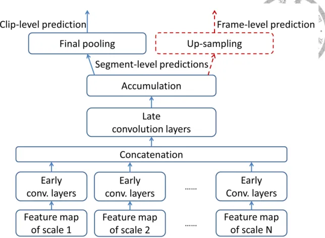
The general structure of the proposed network is depicted in Figure 3.2. According to our design, the proposed model can make both clip-level and frame-level predictions.

The details are provided in what follows.

3.1.1 Clip-level Prediction

As Figure 3.2 shows, the input layer consists of log mel-spectrogram with N different STFT window sizes [14]. As these are frame-level features computed over time, we refer to a log mel-spectrogram computed with a given window size as a feature map. Then, each feature map is processed by its own stack of alternating convolutions and max poolings, referred to altogether as the early convolution layers. Max pooling is applied only along the time axis (but not the frequency axis) for every S frames, which is referred to as the

(41)

Figure 3.2: The proposed FCN architecture. Given a trained network for clip-level prediction (the blue one), we replace the final pooling layer by an up-sampling layer for frame-level prediction (the red component).

stride size. All stacks of early convolution layers in the proposed FCN structure have the same number of layers. The outputs of the last early convolution layers are concatenated together into one feature map, which aggregates information from different scales. This united feature map is fed into another stack of convolutions, referred to as the late con- volution layers. The late convolution layers use only convolutions with no strides (i.e., S = 1) and no max poolings. They provide the function of fully connected layers com- monly used in conventional CNNs and have the benefit of efficiently scanning through a time sequence of arbitrary length. The output of the last late convolution layer is then pro- cessed by a Gaussian filter across time to create the segment-level predictions. A segment would contain multiple frames, because of the previous max pooling layers. If the σ in the Gaussian is trainable in the training phase, we call it “adaptive Gaussian filter”; otherwise, we call it “fixed Gaussian filter.” Finally, the segment-level predictions are pooled over time with the final pooling layer to become one clip-level prediction.

(42)

To facilitate the later discussion, we define the notion of total stride size as the product of all the stride sizes in a stack of early convolution layers. It can be shown that the number of frames covered by a segment in our model equals the total stride size.

3.1.2 Frame-level model

Given a trained network for clip-level prediction, only the last layer is modified to make it possible to make frame-level predictions, as illustrated also in Figure 3.2. There- fore, as there are no trainable parameters in the last layers, the parameters of all layers are shared among the networks for making clip- and frame-level predictions.

Specifically, the aforementioned final pooling layer is now replaced by a up-sampling layer to recover frame-level predictions from segment-level predictions. Two methods of up-sampling are investigated in this paper. The first method is upscaling, which simply repeats the segment-level predictions locally such that the final output has the same number of frames as the input. For example, suppose there are two early convolution layers and each of them has stride size 2. The total stride size is then 4. Accordingly, the output, say [0, 1, 0], of the accumulation layer has to be repeated 4 times, that is, [0, 0, 0, 0, 1, 1, 1, 1, 0, 0, 0, 0].

The second method is patching, which has been used in related work in computer vision [9, 82, 83]. Assuming that the total stride size is 4, two temporally neighboring points in the segment-level result can be seen as being 4-frame apart. To fill the values in between, we can simply shift the audio input 4 times and feed each of them to the FCN.

This might be more accurate than the upscaling method, but obviously it is computationally much more expensive.

Thresholding

An important issue not depicted in Figure 3.2 is the necessity to apply a thresholding on the frame-level predictions to get binary decisions. This is because the output of FCNs lies in the range between 0 and 1 but we may need binary decisions to evaluate the prediction accuracy. As the optimal threshold values may be tag-dependent, the values

(43)

are empirically tuned in the following brute-force way by using validation data (see Sec- tion 4.3). First, we divide the output range [0, 1] into K threshold candidates, namely {0, 1/K, 2/K, ..., (K − 1)/K}. For each music event, the F1 scores (i.e., the harmonic mean of precision and recall rates) of frame-level prediction scores are computed with respect to all the threshold candidates, and the candidate with the highest F1 score is se- lected.

3.2 Data: MagnaTagATune and MedleyDB

We will use two datasets: MagnaTagATune for clip-level training, and MedleyDB for frame-level evaluation.

MagnaTagATune is a music dataset containing clip-level tag annotations [17]. Through letting human subjects play a game, the clips in the dataset were annotated by collecting the human evaluations of music tags generated by an algorithm. It includes 25,863 29- second clips, annotated with 188 tags. The tags include instruments such as “guitar” and

“flute,” genres such as “Jazz” and “new age,” tempo such as “slow” and “fast,” and acoustic properties such as “silence” and “noise.”

MedleyDB is a multi-track instrument dataset [18]. It has instrument annotations and the corresponding F0 annotations at the frame level, so it can be used for research of melody extraction and source separation. It includes 122 multi-track clips and totally 81 instrument tags. The timestamps of instrument activations are provided in terms of starting and ending points, from which we can derive frame-level annotations. In this chapter, the multiple tracks of a clip are merged into one channel.

As there are no music auto-tagging dataset that contains frame-level annotations, I found that a multi-track instrument dataset like MedleyDB is especially suitable for evaluating the performance of music event localization. Common music auto-tagging datasets also contain a rich number of instrument tags. In our case, MagnaTagATune and Med- leyDB have 46 tags in common. In addition, the multi-track audio of instruments in MedleyDB is also in line with the multi-label nature of music auto-tagging. Therefore, I propose to use MedleyDB for evaluating frame-level result.