黏性流體中數值波浪模式之發展及其應用

(1)

※※※※※※※※※※※※※※※※※※※※※※※※※

※ ※

※ 黏性流體中數值波浪模式之發展及其應用 ※

※ ※

※※※※※※※※※※※※※※※※※※※※※※※※※

計畫類別：■ 個別型計畫 □ 整合型計畫計畫編號：NSC

90-2611-E-006-002-

執行期間：

2001

年

08

月

01

日至

2002

年

07

月

31

日

計畫主持人：黃清哲副教授共同主持人：

計畫參與人員：張興漢、林俊遠、王豪偉、沈茂霖

本成果報告包括以下應繳交之附件：

□赴國外出差或研習心得報告一份

□赴大陸地區出差或研習心得報告一份

□出席國際學術會議心得報告及發表之論文各一份

□國際合作研究計畫國外研究報告書一份

執行單位：

國立成功大學水利及海洋工程學系（所）

中華民國 91 年 10 月 31 日

(2)

ABSTRACT

In here, author proposed a new technique to separate the incident and reflected higher harmonic waves using four or more spatially separated probes. Both the free and locked modes in the higher harmonics of the regular waves can be discriminated. The complex waves were decomposed into each frequency component using the Fourier transform. The method of least squares was applied to minimize the possible signal noise and to obtain the equations for solving the unknown parameters related to the wave amplitudes.

The accuracy of this method was verified by using it to resolve the artificial waves with given amplitudes. To demonstrate the applicability, the free surface elevation data collected from probes located upstream and downstream of a submerged breakwater in a numerical wave tank were analyzed. The results were compared with those obtained by using the methods of Goda and Suzuki (1976) and Mansard and Funke (1980). The comparison showed that this method gave more reasonable resolution of the incident and reflected higher harmonics than the other two methods.

摘要

本文主要是發展利用四支波高計分離入反射波的方法，高倍頻波中之自由波及強制波振幅皆能分離出來。本方法利用 Fourier 轉換分離出複合波中各倍頻波，再應用最小二乘法分別求得主頻波中入反射波之振幅，及高倍頻入反射波中自由波及強制波之振幅。利用本方法解析人為給定的波浪時序列資料，可得到與原先給定的各階倍頻波完全相同的入反射波振幅。而 Goda and Suzuki (1976)及 Mansard and Funke (1980)的方法無法正確求出高倍頻波中各成份波之振幅。最後本文示範如何利用本方法求出波浪通過潛堤時，各階入反射波之振幅，並求出反射率。

計畫緣由與目的

The interaction of waves and offshore structures was frequently investigated in a laboratory wave flume or simulated using numerical models. To understand the characteristics of the generated wave fields, it is quite often required to separate out the incident and the reflected waves. A precise description of the incident and the reflected waves would provide also information for analyzing the nonlinear energy transfer from the fundamental waves to the higher harmonics. In the real applications, the incident waves may be random or regular, and the interaction between the waves and structures may produce higher harmonics involving the free mode (free waves) and the phase-locked modes (bound waves).

Furthermore, the offshore structures may be located on a sloping beach with complicated bathymetry or currents. It is difficult to take all of these aspects into account within a single method for resolving the complicated wave fields. Hence, different compromises were made in different methods.

This paper begins with a general expression of the composite waves, involving the free and locked modes in the higher harmonics and an error function. The complex waves were then decomposed into each frequency component using the Fourier transform. The method of least squares was applied to minimize the possible signal noise and to obtain the equations for solving the unknown parameters related to the wave amplitudes. To avoid the singularity in the calculation, condition for the spacing between the probes was provided. For practical applications, procedures for implementing this method were summarized.

Finally, verification and application of the present method were demonstrated.

結果與討論

The main assumption underlying the

analysis of wave decomposition is that the

regular waves can be described as a linear

superposition of an infinite numbers of

discrete components each with its own

frequency, wave height, phase difference

(3)

in the higher harmonics, are also interpreted, the time series data of the surface elevation

) , ( x

m

t

η at each location x

m

in a wave flume can be written as:

) , ( x

m

t

η = a

_I⁽¹⁾

cos( kx

_m

− ω t + φ

_I⁽¹⁾

) )

cos(

⁽¹⁾

) 1 (

R m

R

kx t

a + ω + φ

+

∑

≥

− + +

2

) (

, )

(

,

cos[ ( ) ]

n

n B m I

n B

I

n kx t

a ω φ

∑

≥

+ + +

2

) (

, )

(

,

cos[ ( ) ]

n

n B m R

n B

R

n kx t

a ω φ

∑

≥

− +

+

2

) (

, )

( ) (

,

cos[ ]

n

n F m I

n n

F

I

k x n t

a ω φ

∑

≥

+ +

+

2

) (

, )

( ) (

,

cos[ ]

n

n F m R

n n

F

R

k x n t

a ω φ

+ e

m

(t )

where a is the amplitude and the subscripts I and R denote the incident and reflected waves or can generally be defined as progressive wave trains moving in the same and opposite directions as the incident waves. The second subscripts B

and F denote the bound wave (locked mode) and the free wave (free mode) components, respectively. The superscript

n ( n = 1 , 2 ,...) denotes the nth-harmonic waves. ω is the angular frequency and equal to 2π / T , where T is the fundamental period of the incident waves. k and k

⁽ⁿ⁾

represent the wave numbers of the first-harmonic (fundamental) and the higher harmonics, respectively. φ

⁽ⁿ⁾

is the phase difference related to an arbitrary time origin.

(t )

e

_m

is the error due to the signal noise of the measurement or the extraordinary terms due to the nonlinear wave interactions, such as the evanescent modes, etc..

To verify the accuracy of the present method, we apply it to resolve the artificial wave fields with the given amplitudes in each mode. In order to be as general as possible, the wave fields contain both the incident and the reflected waves and the higher harmonics involve the free and locked modes. The mathematical expression of the wave fields can be written as Eqs.above, and the fundamental wave period of the artificial waves is T = 1 . 0 sec , the still water depth h

_o

= 0 . 4 m . The detailed amplitudes of each mode are listed in Table 1.

Amplitudes Given Unit : (cm)

Goda and Suzuki (1976)

Mansard and Funke

(1980)

Present method

)

1 (

a

I

1.200 1.200 1.200 1.200

) 1 (

a

R

0.400 0.400 0.400 0.400

) 2 (

,B

a

I

0.300 ---- ---- 0.300

) 2 (

,F

a

I

0.100 0.174 0.034 0.100

) 2 (

,B

a

R

0.090 ---- ---- 0.090

) 2 (

,F

a

R

0.060 0.294 0.104 0.060

) 3 (

,B

a

I

0.050 ---- ---- 0.050

) 3 (

,F

a

I

0.030 0.263 0.053 0.030

) 3 (

,B

a

R

0.020 ---- ---- 0.020

) 3 (

,F

a

R

0.010 0.045 0.055 0.010

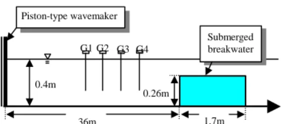
The present method can be applied to decompose the composite waves generated in a laboratory wave flume or obtained in the numerical simulations. For our convenience, we will demonstrate the application of this method to resolve the wave fields generated in the interaction of waves and a submerged breakwater in a numerical wave tank developed by Huang et al. (1998) and Huang and Dong (1999 and 2001).In the numerical wave tank, a piston-type wavemaker is set up to produce the incident waves. A rectangular breakwater of width b = 1 . 7 m and height

m

h = 0 . 26 is installed at the bottom of the tank, with a distance of 36 m from the left edge of the breakwater to the wavemaker.

Figure 1 shows a schematic diagram of a submerged breakwater located at the bottom of a two-dimensional numerical wave tank.

The still water depth of the tank is 0 . 4 m . The incident wave period is T = 2 . 5 sec

and wave height H

_i

= 2 . 5 cm . This corresponds to an Ursell number of U

r

= 8 . 77 ,

G1G2 G3 G4

36m 1.7m

0.4m

0.26m

Submerged breakwater Piston-type wavemaker

Fig. 1. Schematic diagram of a breakwater located at

the bottomof a 2-dimensional numerical wave tank.

(4)

40 41 42 43 44 45 46 47 48 49 50 t (cm) -2.0

-1.0 0.0 1.0 2.0

η(cm)

Fig. 2. Purely incident wave recorded at x = 27 m

which indicates the nonlinearity of the waves. For making sure that the separated incident waves are correct, the same numerical wave tank was separately run without the breakwater. Figure 2 shows the incident waves recorded at x = 27 m in the numerical wave tank without the breakwater.

To resolve the waves, ten wave gauges were distributed from x = 26 . 7 m to

m

x = 27 . 24 with equal spacing ∆ x = 6 cm . Among the ten available probes, we collect the free surface elevation data from four arbitrarily chosen probes. The detailed wave amplitudes obtained using the present method were presented in Table 2.

Figure 3 shows the waves recorded at

m

x = 27 in the numerical wave tank as Stokes waves propagating over a submerged breakwater. With the same wave gauges allocation and the same data acquisition method as the previous case, the detailed wave amplitudes obtained using the present method are presented in Table 3. This location is upstream of the breakwater. The recorded waves are composed of the incident waves and the reflected waves from the breakwater.

Table 2. Decomposition of the purely incident Stokes waves in a numerical wave tank at x = 27 m .

Amplitude Unit :(cm)

Goda and Suzuki (1976)

Mansard and Funke (1980)

Present method

) 1 (

a

I

1.27 1.27 1.27

) 1 (

a

R

0.00 0.00 0.00

) 2 (

,B

a

I

--- --- 0.13

) 2 (

,F

a

I

0.12 0.12 0.01

) 2 (

,B

a

R

--- --- 0.00

) 2 (

,F

a

R

0.01 0.01 0.00

) 3 (

,B

a

I

--- --- 0.01

) 3 (

,F

a

I

0.01 0.01 0.01

) 3 (

,B

a

R

--- --- 0.00

) 3 (

,F

a

R

0.00 0.00 0.00

K

R

0.0 % 0.0 % 0.0 %

40 41 42 43 44 45 46 47 48 49 50

t (cm) -2.0

-1.0 0.0 1.0 2.0

η(cm)

Fig. 3. Stokes waves recorded at x = 27 m .

The separated incident wave amplitudes in Table 3, namely a

_I⁽¹⁾

, a

⁽_I²_,B⁾

,

) 2 (

,F

a

I

, a

I⁽³,B⁾

and a

I⁽³,F⁾

, are exactly the same as those in Table 2. The results in Table 3 show that the reflected waves contain mainly the first harmonic. The second harmonic waves, which involve both the free and locked modes, are rather minor. We note also that the present method gave exactly the same first harmonic incident and reflected wave amplitudes as those obtained by the method of Goda and Suzuki (1976) and Mansard and Funke (1980). In addition, the free and bound waves in the higher harmonics can be discriminated by the present method. In spite of the different higher harmonic wave amplitudes, the resultant reflection coefficients are identical among the three methods, as the dominant wave energy are about the same.

The demonstration given in this section indicates that the present method gives exactly the same first harmonic incident and reflected waves amplitudes as those obtained by the methods of Goda and Suzuki (1976) and Mansard and Funke

Table 3. Decomposition of the waves generated in a numerical wave tank at x = 27 m as Stokes waves

propagating over a submerged breakwater.

Amplitude Unit :(cm)

Goda and Suzuki (1976)

Mansard and Funke (1980)

Present method

) 1 (

a

I

^1.27 ^1.27 ^1.27

) 1 (

a

R

0.51 0.51 0.51

) 2 (

,B

a

I

--- --- 0.13

) 2 (

,F

a

I

0.12 0.12 0.01

) 2 (

,B

a

R

--- --- 0.05

) 2 (

,F

a

R

0.07 0.07 0.07

) 3 (

,B

a

I

--- --- 0.01

) 3 (

,F

a

I

0.01 0.02 0.01

) 3 (

,B

a

R

--- --- 0.00

) 3 (

,F

a

R

0.02 0.02 0.02

K

R

16.3 % 16.3 % 16.4 %

(5)

waves in the laboratory experiments nowadays. Furthermore, the full modes in the higher harmonics can be determined by the present method. This will provide information for understanding the nonlinear interaction between waves and structures.

計畫成果自評

This paper extended the method of Mansard and Funke (1980) to separate the incident and reflected higher harmonic waves using four or more wave gauges.

Examination of this technique with wave tests shows the followings:

(1) This technique is able to decompose the regular wavefields into their full modes, including the free waves and the bound waves in the higher harmonics.

(2) The formulations developed in the text of this paper are suitable for four or more spatially separated probes.

(3) Accuracy of this technique was verified and the applicability of this technique was demonstrated.

參考文獻

[1] Baldock, T. E. and D. J. Simmonds (1999) “Separation of incident and reflected waves over sloping bathymetry,” Coastal Eng., Vol. 38, pp.

167-176.

[2] Brossard, J., A. Hemon and E.

Rivoalen (2000) “Improved analysis of regular gravity waves and coefficient of reflexion using one or two moving probes,” Coastal Eng., Vol. 39, pp.

193-212.

[3] Dong, C. M. and C. J. Huang (2001)

“On a 2-d numerical wave tank in viscous fluid,” Proc. of the 11th Int.

Offshore and Polar Eng. Conf., Vol. III, pp. 148-155.

incident and reflected irregular waves,”

Coastal Eng., Vol. 24, pp. 205-215.

[5] Goda, Y. and Y. Suzuki (1976)

“Estimation of incident and reflected waves in random wave experiments,”

Proc. 15th Costal Eng. Conf., ASCE, pp. 828-845.

[6] Huang, C. J., E. C. Zhang and J. F. Lee (1998) “Numerical simulation of nonlinear viscous wavefields generated by a piston-type wavemaker,” J. Eng.