2004 IEEE International Conference on Systems, Man and Cybernetics
Adaptive Tracking Control for a Class of Non- autonomous Systems Containing Time-varying
Uncertainties with Unknown Bounds *
Po-Chang C h e n a n d An-Chyau H u a n g Deparhnent of Mechanical Engineering National Taiwan University of Science and Technology
43, Keelung Road, Sec. 4, Taipei, Taiwan iD9103403, achuang) @mail.ntust.edu.tw
Abstract - This paper proposes an adaptive tracking controller based on function approximation technique (FAU f o r a class of M M 0 non-autonomous systems with time-varying uncertainties. Since it is assumed that the variation bounds of some of the uncertainties are unavailable, conventianal robust strategies camiot be applied Besides, due to /heir time-varying nature, traditional adaptive schemes are iirjeasible. In this paper, an adaptive controller is developed f o r Mh40 square systems such that bounded trackirig pe$ormance can be obtained and the singulari~~ problem of the control input can be totally uvoided. ifthe bounds of the uncertainties in the inpuf-coupling matrix are mailable. Rigorous proof of the closed-loop stability and the performance analysis af the transient state are derived based on the Lapunov-like approach. Some simulation examples are performed to v e r ~ the effectiveness of the proposed method
Keywords: Adaptive control, function approximation, non-autonomous system.
1 Introduction
A large amount of researches have been devoted to maintain the control performance under a variety of system uncertainties as well as external disturbances. Two main approaches for coping with this kind of problems are robust control and adaptive control. However, most of the robust control strategies require that the uncertainties be defined in some known compact sets. On the other hand, almost all adaptive control schemes are restricted to the system with constant or slowly time-varying parameters.
For the system with general uncertainties, i.e. time-varying uncertainties with unknown bounds, those two approaches may not he applicable. Furthermore, since those uncertainties might be in the input channel, the singular problem of the control input [4,10] should be well considered. To deal with these problems, several approaches based on FAT have been proposed for SISO uncertain systems with satisfactory results [l-61. However, for the control of MIMO uncertain systems, due to the
coupling among various inputs and interconnected states among subsystems, the control problem becomes more complex and difficult than that in SISO case. To handle this, Spooner and Passino [8] suggested an indirect adaptive controller for an unknown square decentralized system without any input coupling. Further researches on dealing with input coupling effects were made by Ordonez and Passino in [9] where the projection algorithm was employed to keep the estimated parameters inside a convex set to avoid the singularity problem. However, to implement the controller, not only should the convex set be constructed a priori but some strict assumptions for the unknown input gain as those in [I] are also necessary for the diagonal elements in the uncertain input-coupling matrix. A neural network based adaptive control algorithm was developed by Ge et a1 [IO] for nonlinear MIMO systems with a triangular control structure. By using the triangular property, the control singularity problem is prevented and bounded tracking with guaranteed transient performance is obtained. In [ll], Zhang et a1 attempted to use the fuzzy basis function vector method to adaptively estimate the bounds of the uncertainties such that the controller can give asymptotic tracking performance, if the uncertainty in the input-coupling matrix is invertible and a sufficient number of fuzzy bases can be used in approximation with desired accuracy. A new robust adaptive controller using neural networks with breakthrough results was proposed by Xu and Ioannou [12].
In their approach, only some simpler assumptions on unknown vector fields and system controllability should be satisfied and then global stability of the closed-loop system with steady-state error bound can be obtained. However, to amve at this goal, a key-information, the bounds of the approximation errors, should be known, or bounded tracking may not be ensured.
In this paper, we would like to propose an adaptive tracking controller based on FAT for a class of uncertain MIMO non-autonomous systems. Since the systems are assumed to have general uncertainties, traditional adaptive schemes or robust strategies may not be applicable. The
FAT [1-6,8-121 is thus used to represent those time-varying uncertainties as linear combinations of basis functions with unknown constant coefficients, and then the parameter update laws are chosen to ensure the closed-loop stability.
Rigorous stability proof and performance analysis of transient states are made using Lyapunov-like direct method It is proved that bounded tracking errors with stahle closed-loop system can he guaranteed with the proposed controller, and the singularity of the control input can be completely avoided, if the bounds of the input- coupling matrix are available.
This paper is organized as follows. Section 2 derives the proposed adaptive controller io detail. Some simulations are performed in Section 3 to verify the effectiveness of the proposed method. Section 4 concludes this paper.
2 Main results
An uncertain square system composed of m subsystems whose orders are respectively nj , i = l , . . . , m , can be represented as
(1)
$J = f , ( X , l ) + ~ g , ( X , f ) u j + d , ( t )
j = l
yi = x i i = l ... m
1 "i
1 , I
where X = [x; x: . . . x i r E 31 ' is the measurable state vector with xi = [xi i, . . . .p-I)r E :%". , yi is the output of the ith subsystem, u j E 111 is the control input, f, is an unknown continuous function with unknown bound, and g, is the unknown input gain. The extemal disturbance d , is assumed to be an unknown continuous function whose variation bound is not available either. It can be observed that each subsysteni is interconnected via system vector field f, and the control inputs are coupled if the input gains g, # 0 for i f j .
Dejinition2If S, E W for i=l;..,n,then ~ ~ ~ ~ ~
Define F = h i, ... imp EM'" with 7, =f, + d , ,
-
G={gr}~IJ1""" , x = [ x p - l ) ~ ( " * - l ) 2 _.. x$-')p = M m and U = [ u , U, ... um]' E M I , and then (I) can be rewritten as
% = F + G U (2)
Assumption 1: G is nonsingular with gji # 0 i = 1;'. , m , for all I and its uncertainties in multiplicative form can be represented as
G = (I+A)G, (3)
where G , E 3"""' is the invertible nominal matrix and A = {A,}. %" is the uncertain matrix with ( A I ( S 6, for i, j = I,...,m , for some known values 6, > 0 satisfying llDll, < I with D=(~,}E!W'""'.
The objective is to design a controller such that the system output y, = xi can track the desired trajectoly x,,, (1) , for i = I,. . . , m . However, since the bounds of the unknown time-varying function i, (X, I) are unavailable, both robust strategies and adaptive schemes are infeasible. Here, we would like to use FAT [S-61 to represent as linear combinations of basis functions as
f i = w ? q - /, fi + E - , L i = l ; . . , m (4)
where 'pi, = 4, ... @ni, p E %"', is the vector of basis
functions and p E%"', is its
unknown coefficient vector to be estimated. The positive integer n - is the number of terms of basis functions used in approximation and E - - x w j @ j is the bounded approximation error due to finite-term ap roximation.
Supposing that an identical number n5 2 max i. of basis functions are used to represent each and every entry in F , then we have
wi = [w, w 2 ...
wai.
L
a
- i=";*,
JI
= w p , + E i ( 5 )
A i =
where W, = diag(w - , w - ;.., w - ) E %-"" with wi: €97- , S=br A cpr A ... rpr f. ~ E ! N " ' ~ with
'pi, ~'.l?- and &,=[si; E - x ... E ~ ~ ~ E % " ' . Let the tracking errors be e, = x , -qd i = 1, ...,m , and the synthesized error vector be .=[e: e! ... e i p ~ 9 7 ~ " ' with e, =[er e, ... e!'-I)T E 97". and then the control law can be designed according to (2) and (5) as
X h .1
U = G:[-W& +v -q sgn(B'PE)] (6a) q = (I-D)-'Dabs(-W;% + v ) (6b) where W, E%"-'"' is the estimate of W, , v = [v, v2 ... v,]' ~ 9 is the vector of desired 7 ~
0 1 0 .(.
0 0 1 ."
!
0 0 0 .'.
i
1 ]r!,7",x_ Since l/D112 < 1 , according to the Frobenius-Perron theorem - k i , -k,, - k i 2 ... - k . [7], given any k E 9im with non-negative elements, theref(-,-l)
. . . .
Lemma I: Let a=[., a2 ... am]' E W and c=[c, c, '.. cm]' , and uncertain matrix be A = {A?} E %"", If Assumption 1 holds, then given any k = [ k , k, ... k,Ir with ki 2 0 for all i, there exists a q E %"' whose elements are all non-negative such that
a'[-(I+A)(g sgn(a))+Ac]< -(abs(a))'k 2 0 (8) Moreover, q can be calculated by
q =(I-D)-'Dabs(c)+k (9)
Prooj Supposing that q = [ a 7, ... q , r , the left hand side of (8) can be written as
a'[- (I +A)(q sgn(a))+Ac] =
The ith element in the summation of (IO) can be derived to be
(F"+
B = diag(b,,b,,...,b,) E 97
m
- (1 - St,)vj + c S v v j + c S g l c j l = -kj , i = 1 , . . . , m (12)
with j r i j = l
" I", b, = [o 0 ... 11' E 97"' , and p = P T E !17(f ' ) ( ' is a positive defmite matrix satisfying the Lyapnnov equation
+ PA = -Q for A = diag(A, ,A,,. ..,A,) and for Q = Q' > 0. With the control law in (6), system (2) can be written as the error dynamics driven by parameter errors
E=AE+B[6'&+A(-Wi++v)
Moreover, q can be computed by (9). Q.E.D.
Theorem I: Given a set of sufficiently smooth desired trajectories x d i = I;..,m , for the system (2) under Assumption 1, if the control law and the update law for
Wi are respectively designed as (6) and
-(I+Ap1 sgn(B'PE)+& (7) wF = r l ( y r PB- hF) (13)
where W, - = W, - W, . where r E ~ ( m " i ' x ~ m " ? ) IS ' positive definite and cr E 9i is
candidate V with the initial condition V, at / = I , is chosen as
V = E'PE + Tr(%'ir6JF) ( 14)
then the transient bound of E for f 2 1, can be derived as
(15) where yii , i = 1;. . , mng are diagonal elements of r and
With (18a) and (18b), it is easy to write (17) as
where n>O is chosen as the form in (15) so that a V 5 7 ~ m j n ( ~ ) ~ ~ ~ ~ ~ ~ + o ~ r ( G i f + ~ ) . This implies V S o
for all 1
Prooj In order to show the boundedness of the [:mor signals in (71, we can choose Lywnov-like function candidate as (14) and take its time derivative along (?) to obtain
Therefore, error signals E and %, are uniformly bounded.
Using the comparison lemma, the transient bound of V for I I, can be computed as
Therefore, the bound of E can be derived as the form of (15). Q,E,D.
Remark I : If na is chosen to be sufficiently large so that
E 0 , then the positive constant c in (13) may be set to If the update law for Wi and the parameter q are chosen
as (13) and (6b), respectively, then according to Lemma I , (16) becomes
~ 5 - E ' Q E + 2 o T r ( % ' ~ W s ) + 2 E ' P B ~ , (17) zerotohave Since W, = W, - %'r , the following two inequalities can
be derived form the right-hand side of (17) as -E'QE + ZE'PBE,
5 -.l-i.(Q)IIEll: +~JIPBEBI~,$II~ ( 184
v 5 -E'QE
I
This implies E EL, n L, , and W, E L, . Besides, from (7), it can he easily verify that E E L, . Hence, according to the Barbalat's lemma, we may conclude that tracking error
E+O as f + m ,
Remark 2: If E cannot be ignored but its variation bound is available [l-4,8-121, i.e. 3 f l > 0 such that It i(12 5,B
for all I 2 0 , then q in (6b) can be modified with an additional term p = [p p , , . p r E 171" as
1 =(I-D)-'Dabs(-Wi% + v ) + p
If we choose the control law as (6a) and the update law as (I 3) with U = 0 , then according to Lemma 1, f becomes
f s - E r Q E + 2 ( a b s ( B r P E ) ~ ( ~ B - p ) < 0 Therefore, asymptotic convergence of tracking error can still be concluded using Barbalat's lemma.
3 Simulation examples
To verify the effectiveness of the proposed method, some computer simulations are performed to an uncertain square system composed of two subsystems respectively with orders n1 = I and n, = 2 , with the following structure
1
1
- - x , I x , I + i , sin(x,)+5sin(151) - i: - x, - 3x, + 3sin(20t) 2 +OSsin(/) -0.5+cos(2f) 1+0.7sin(31) l-0.25cos(f) F = [
G = [
where xI and x2 are the outputs of the 1' and Zd subsystems, respectively. Since the bounds of the uncertainties in G are available, matrices G , and D can be comouted according to Assumotion 1 as G , = [i .-y] and D
=p
0.4 0.35 . Cbntroller gains are chosen as k,, = 2 , k,, = 25 and k,, = 7 . To avoid chattering in the control action, the sgn(s) function in (6a) is replaced by the saturation function sat($/@) with the boundary layer thickness 4 = 0.1 . The first 11 terms of the Fourier series is employed as the basis functions to represent both A and 7, in (5). A diagonal matrix whose elements are equal to IO4 is chosen as the gain matrix I' in (13) and Q in the update law is selected as zero. The initial values of the elements in WF(0) are all set to be 0.01, and the initial conditions of the system are with x,(O) =-1 and x,(O)=[2 0 I r . The desired trajectories for two subsystems are respectively designed asxld = 2sin(f) and xZd = -sin(2t).
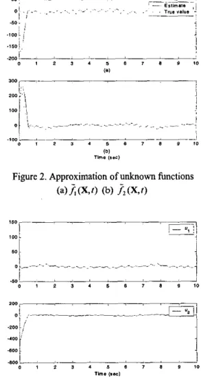
Simulation results are shown in figure 1 to 3. From figure 1, it is observed that system outputs track the desired trajectories nicely regardless of the existence of the system uncertainties. Figure 2 presents the function approximation performance for the unknown functions and 7, . Figure 3 gives the time histories of the control inputs to show the feasibility of the proposed method.
Figure I. System output trajectories ( J'; = x i , i = 1,2)
/-,
rl"a / I * G )
Figure 2. Approximation of unknown functions (a) (X, I ) (b) .6 (X, 0
4 Conclusions
In this paper, we have proposed a new adaptive controller based on FAT for a class of uncertain MIh40 square non-autonomous systems. To ensue the closed-loop stability, rigorous proof based on the Lyapunov-like direct method is derived. Although the system contains genua1 uncertainties, the proposed method can still give satisfactory tracking performance without singulaiity problem. Furthermore, simulation results show that the proposed method can be implemented with realizable control efforts.
Acknowledgement
This research was partially supported by the Natianal Science Council of the Republic of China govemment under the contract number: NSC92-2212-E-011-018.
References
[I] J.T. Spooner and K.M. Passino, “Stable adapi:ive control using fuzzy systems and neural networks,” IFEE Trans. Fuzzy S j ~ t . , vol. 4, no. 3, pp. 339-356, 1996.
[2] J.T. Spooner, M. Maggiore, R. Ordonez and K.M.
Passino, Stable Adapfive Confrol and Estimation far Nonlinear Systems - Neural and Fuzzy Approximiifor
Techniques, Wiley, New York, 2002.
[3] S.S. Ge, C.C. Hang and T. Zhang, “A direct method for robust adaptive nonlinear control with guaranteed transient performance,” Sysf. Contr. Left., vol. 37, pp. 275- 284,1999.
[4] S.S. Ge, C.C. Hang, T.H. Lee and T. Zhang, Sfoble Adapfive Neural Newark Control, Kluwer Academic Publishers, 2002.
[5] A.C. Huang and Y.S. Kuo, “Sliding control of nonlinear systems containing time-varying uncertairdies with unknown bounds,” Inf. J. Contr., vol. 74, no. 3, pp.
252-264,2001.
[6] A.C. Huang and Y.C. Chen, “Adaptive Multiple- Surface Sliding Control for non-autonomous systems with mismatched uncertainties,” Aufomafica, in press.
[7]
Wiley, New York, 1979.
[8] J.T. Spooner and K.M. Passino, “Adaptive control of a class of decentralized nonlinear system,” IEEE Trons.
Automaf. Contr., vol. 41, no. 2, pp. 280-284, 1996.
D.G Luenberger, Infroduc/ion io Dynamic Systi.ms,
[9] R. Ordonez and K.M. Passino, “Stable multi-input multi-output adaptive fuzzylneural control,” IEEE Trans.
Fuzzy Sysf., vol. 7, no. 3, pp. 345-353, 1999.
[lo] S.S. Ge, C.C. Hang and T. Zhang, “Stable adaptive control for nonlinear multivariable systems with a triangular control structure,” IEEE Trum. Aufomaf. Contr., vol. 45,no. 6,pp. 1211-1225,2000.
[ I l l H.G. Zhang, L.L. Cai and Z.G. Bien, “A fuzzy function vector-based multivariable adaptive controller for nonlinear systems,” IEEE Trans. Sysf., Man, Cybem., vol.
30, no. 1, pp. 210-217,2000.
[I21 H. Xu and P.A. Ioannou, “Robust adaptive control for a class of MIMO nonlinear systems with guaranteed error bounds,” IEEE Trans. Aufomaf. Confr., vol. 48, no. 5 , pp.
728-742,2003.