結構最佳化之兩點適應移動漸近線近似法

國立臺灣大學工學院機械工程學研究所 碩士論文

Department of Mechanical Engineering College of Engineering

National Taiwan University Master Thesis

結構最佳化之兩點適應移動漸近線近似法 Two-Point Adaptive Method of Moving Asymptotes

Approximation for Structural Optimization

陳峰遠

Fong-Yuan Chen

指導教授：鍾添東 博士 Advisor: Tien-Tung Chung, Ph.D.

中華民國 106 年 7 月

July 2017

誌謝

本論文得以完成，首先要感謝指導教授鍾添東老師，在我研究所求學過程中 的細心教導與諄諄教誨，讓我獲益良多。同時也感謝口試委員林陽泰老師與史建 中老師在專業上的指教與建議，使本論文更臻完善。

在這兩年的求學生涯中，感謝電腦輔助繪圖實驗室的全體成員。感謝浩宇學 長引領我進入結構分析以及結構最佳化的研究，並在研究過程中給予指導，即使 畢業也會撥空回答並協助解決研究上遇到的各種難題。感謝同窗騰輝、承楷、期 文，在課業與研究上提供的支援與協助，並相互陪伴撐過許多難關。以及維德、

尚哲、慶雄、永健、以磬、承林、子皓、育菁、郁寬、志承與晟右平時的協助與 關心。

另外，感謝好友煥庭、暐凱。雖然大家各奔東西，也不時關心我的研究狀況 並在我心情低落時給予鼓勵和陪伴，讓我的研究生活一路走來更加順暢。

最後感謝我的父母、兄弟以及親人在這一路上的支持與關心，並提供充足的 資源讓我在求學生涯中無後顧之憂，才能順利完成學業。

在此致上最誠摯的感謝。

中文摘要

本研究之目的為改良結構最佳化設計之保守近似法，並根據移動漸近線近似 法發展一種新的兩點近似法，稱為兩點適應移動漸近線近似法。在此方法中，藉 由修改移動漸近線近似法之中介變數來產生斜漸近線，並利用兩連續設計點之函 數值及靈敏度值自動調整斜漸近線之斜率。換言之，本方法會考量結構行為的單 調性來建立近似函數以確保近似品質。另外，本研究提出一種採用分段近似函數 的新修改策略，以避免過往保守近似法中奇異點與不當近似的產生。經由此近似 法，可將結構之行為函數轉換成以設計變數表示的顯函數，如此一來，最佳解便 能透過數學優化法對連續近似最佳化問題加以求解而得到。此研究亦整合最佳化 程式、電腦輔助繪圖軟體及有限元素分析軟體進行自動化結構最佳設計，並以多 個結構最佳化問題驗證本近似法及修改策略。結果顯示，利用兩點適應移動漸近 線近似法可準確而快速地找出最佳解，並且利用修改策略可有效地處理奇異點及 不當近似。這驗證了本研究之理論在結構最佳化中的實用性。

關鍵字：結構最佳化、連續近似最佳化、兩點近似法、保守近似法、中介變數

ABSTRACT

The purpose of this thesis is to improve conservative approximation methods for structural optimization. A new two-point approximation method based on method of moving asymptotes approximation (MMA) is developed, which is called two-point adaptive method of moving asymptotes approximation (TAMMA). It modifies intervening variables of MMA to generate oblique asymptotes and utilizes function values and sensitivities at two successive design points to adjust the slopes of the oblique asymptotes automatically. In other words, it can consider the monotonicity of structural behavior to construct approximate functions to ensure the approximation quality. Also, a new modification strategy which adopts piecewise approximate functions is proposed to avoid the singularity and inappropriate approximation that existing conservative approximation schemes would encounter. With the use of TAMMA, several kinds of structural behavior can be represented as explicit functions of design variables. Therefore, the optimum design can be found with sequential approximate optimizations solved by mathematical optimization techniques. Moreover, a program integrating ANSYS, AutoCAD and Microsoft Visual C++ is developed for automated structural optimization. TAMMA and the modification strategy are tested in several structural optimization problems. The results indicate that TAMMA can converge to accurate optimum designs quickly, and the modification strategy can deal with singularities and inappropriate approximations effectively. Those prove that the proposed methods are practical in structural optimization.

Keyword: Structural optimization, Sequential approximate optimization, Two-point approximation method, Conservative approximation method, Intervening variables

CONTENTS

口試委員會審定書 ...i

誌謝 ... ii

中文摘要 ... iii

ABSTRACT ...iv

CONTENTS ... v

LIST OF FIGURES ...ix

LIST OF TABLES ...xi

LIST OF SYMBOLS ...xiv

LIST OF APPROXIMATION METHODS ...xvi

Chapter 1 Introduction ... 1

1.1 Introduction to structural optimization ... 1

1.2 Paper review ... 2

1.3 Research motivation ... 6

1.4 Outline ... 6

Chapter 2 Application of approximation methods in structural optimization .... 8

2.1 Mathematical optimization procedure ... 8

2.1.1 Selection of design variables ... 8

2.1.2 Definition of objective function ... 9

2.1.3 Treatment of constraints ... 9

2.1.4 Application of approximation methods ... 11

2.1.5 Application of sensitivity analysis ... 11

2.1.6 Application of mathematical optimization ... 12

2.2 Monotonic approximation methods ... 13

2.2.1 Direct linear approximation ... 13

2.2.2 Reciprocal approximation ... 13

2.2.3 Modified reciprocal approximation ... 14

2.2.4 Conservative and convex linearization approximation ... 14

2.2.5 Method of moving asymptotes ... 15

2.2.6 Two-point modified reciprocal approximation ... 16

2.2.7 Two-point exponential approximation ... 17

2.2.8 Two-point adaptive nonlinearity approximation ... 18

2.2.9 Two-point adaptive nonlinearity approximation-1 ... 18

2.3 Non-monotonic approximation methods ... 19

2.3.1 Spherical approximation method ... 19

2.3.2 Two-point adaptive nonlinearity approximation-2 ... 20

2.3.3 Two-point adaptive nonlinearity approximation-3 ... 21

2.3.4 Gradient-based MMA ... 21

2.4 Considered-monotonicity approximation methods... 22

2.4.1 GBMMA-MMA ... 22

2.4.2 Two-point piecewise adaptive approximation ... 22

2.5 Modification for strictly convex approximation ... 24

2.6 Integrated optimization program ... 25

2.7 Integrated sensitivity analysis program ... 26

Chapter 3 The proposed approximation method ... 28

3.1 Two-point adaptive MMA ... 28

3.2 Modification for continuous approximation ... 32

3.3 Numerical tests ... 34

3.3.1 Example 1 ... 35

3.3.2 Example 2 ... 36

3.3.3 Example 3 ... 37

Chapter 4 Optimization of small scale structures ... 39

4.1 2-bar truss optimization ... 39

4.2 3-bar truss optimization ... 42

4.3 4-bar truss optimization ... 44

4.4 6-bar truss optimization ... 46

4.5 10-bar truss optimization ... 49

4.6 25-bar truss optimization ... 51

4.7 Multi-section circular beam optimization ... 54

4.8 Multi-section tube beam optimization ... 56

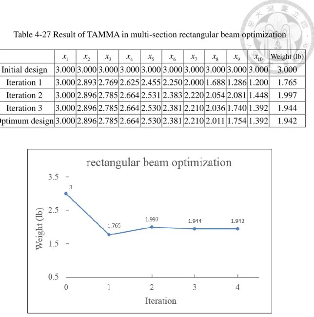
4.9 Multi-section rectangular beam optimization ... 58

Chapter 5 Optimization of large scale structures ... 61

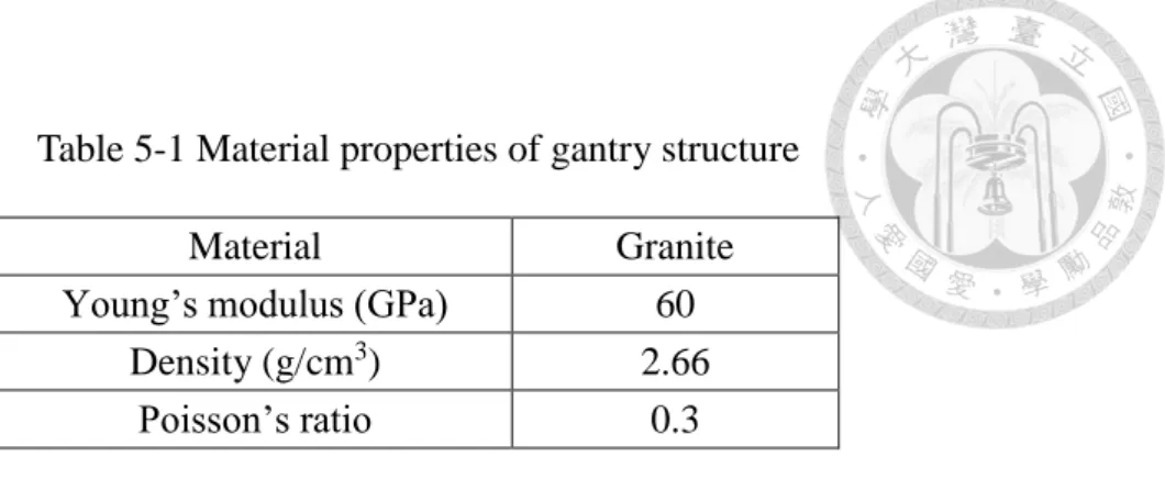
5.1 Optimization of gantry structure ... 61

5.1.1 Self-weight optimization of gantry structure ... 63

5.1.2 Modal optimization of gantry structure ... 65

5.1.3 Combinational optimization of gantry structure ... 67

5.2 Optimization of electric scooter... 69

5.2.1 Drop test optimization of electric scooter ... 72

5.2.2 Double drum test optimization of electric scooter ... 75

Chapter 6 Conclusions and suggestions ... 80

6.1 Conclusions ... 80

6.2 Suggestions ... 81

REFERENCES ... 82

Appendix A: User manual of integrated optimization program ... 86

Appendix B: User manual of integrated sensitivity analysis program ... 90 Vitae ... 93

LIST OF FIGURES

Fig. 2-1 Flow chart of developed optimization program ... 25

Fig. 2-2 Flow chart of developed sensitivity analysis program ... 27

Fig. 3-1 Basic concept of proposed approximation method ... 29

Fig. 3-2 Modification for continuous approximation ... 33

Fig. 3-3 Geometry for 3-bar structure ... 35

Fig. 3-4 Relative error of example 1 ... 36

Fig. 3-5 Relative error of example 2 ... 37

Fig. 3-6 Relative error of example 3 ... 38

Fig. 4-1 2-bar truss structure ... 39

Fig. 4-2 Iteration history of weight of 2-bar truss ... 41

Fig. 4-3 3-bar truss structure ... 42

Fig. 4-4 Iteration history of weight of 3-bar truss ... 43

Fig. 4-5 4-bar truss structure ... 44

Fig. 4-6 Iteration history of weight of 4-bar truss ... 46

Fig. 4-7 6-bar truss structure ... 47

Fig. 4-8 Iteration history of weight of 6-bar truss ... 48

Fig. 4-9 10-bar truss structure ... 49

Fig. 4-10 Iteration history of weight of 10-bar truss ... 50

Fig. 4-11 25-bar truss structure ... 51

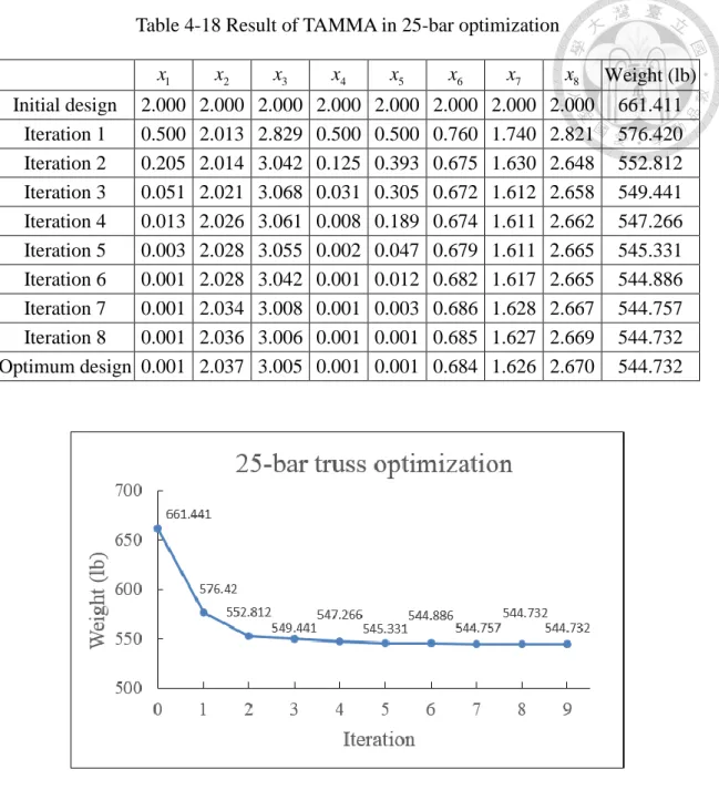
Fig. 4-12 Iteration history of weight of 25-bar truss ... 53

Fig. 4-13 Multi-section circular beam structure ... 54

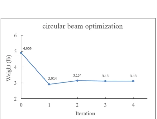
Fig. 4-14 Iteration history of weight of multi-section circular beam ... 55

Fig. 4-15 Multi-section tube beam structure ... 56

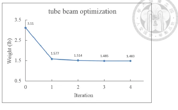
Fig. 4-16 Iteration history of weight of multi-section tube beam ... 58

Fig. 4-17 Multi-section rectangular beam structure ... 59

Fig. 4-18 Iteration history of weight of multi-section rectangular beam... 60

Fig. 5-1 Prototype of wafer inspection stage ... 61

Fig. 5-2 Simplified CAD model of gantry structure ... 62

Fig. 5-3 Selection of design variables for gantry structure... 62

Fig. 5-4 Boundary conditions of gantry structure in self-weight analysis... 63

Fig. 5-5 Iteration history of weight of gantry structure in self-weight optimization ... 65

Fig. 5-6 Iteration history of weight of gantry structure in modal optimization ... 67

Fig. 5-7 Iteration history of weight of gantry structure in combinational optimization .. 69

Fig. 5-8 Components of electric scooter ... 70

Fig. 5-9 Simplified CAD model of electric scooter... 70

Fig. 5-10 Selection of design variables for electric scooter ... 71

Fig. 5-11 Selection of inspection components for electric scooter ... 71

Fig. 5-12 Boundary and loading conditions of electric scooter in drop test analysis ... 73

Fig. 5-13 Iteration history of weight of electric scooter in drop test optimization ... 75

Fig. 5-14 Illustration of double drum test ... 76

Fig. 5-15 Boundary and loading conditions of electric scooter in double drum test analysis ... 77

Fig. 5-16 Iteration history of weight of electric scooter in double drum test optimization ... 79

Fig. A-1 Operation steps of optimization program ... 89

Fig. B-1 Operation steps of sensitivity analysis program...92

LIST OF TABLES

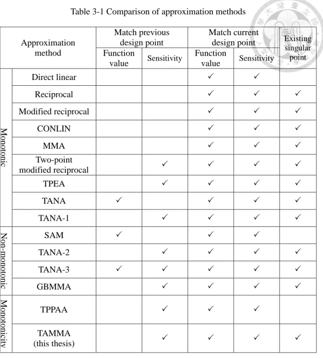
Table 3-1 Comparison of approximation methods ... 32

Table 4-1 Design data for 2-bar optimization ... 40

Table 4-2 Result of TAMMA in 2-bar optimization ... 41

Table 4-3 Result comparison for 2-bar optimization ... 41

Table 4-4 Design data for 3-bar optimization ... 42

Table 4-5 Result of TAMMA in 3-bar optimization ... 43

Table 4-6 Result comparison for 3-bar optimization ... 44

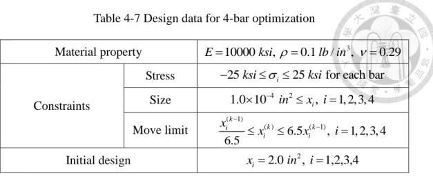
Table 4-7 Design data for 4-bar optimization ... 45

Table 4-8 Result of TAMMA in 4-bar optimization ... 45

Table 4-9 Result comparison for 4-bar optimization ... 46

Table 4-10 Design data for 6-bar optimization ... 47

Table 4-11 Result of TAMMA in 6-bar optimization ... 48

Table 4-12 Result comparison for 6-bar optimization ... 48

Table 4-13 Design data for 10-bar optimization ... 49

Table 4-14 Result of TAMMA in 10-bar optimization ... 50

Table 4-15 Result comparison for 10-bar optimization ... 51

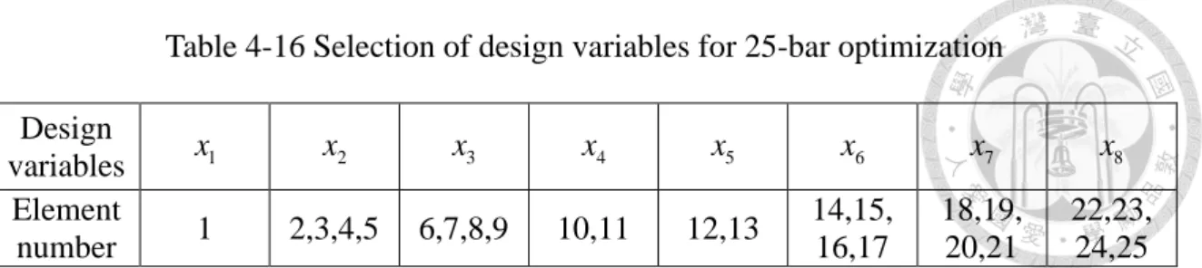
Table 4-16 Selection of design variables for 25-bar optimization ... 52

Table 4-17 Design data for 25-bar optimization ... 52

Table 4-18 Result of TAMMA in 25-bar optimization ... 53

Table 4-19 Result comparison for 25-bar optimization ... 53

Table 4-20 Design data for multi-section circular beam optimization ... 54

Table 4-21 Result of TAMMA in multi-section circular beam optimization ... 55

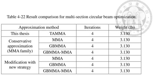
Table 4-22 Result comparison for multi-section circular beam optimization ... 56

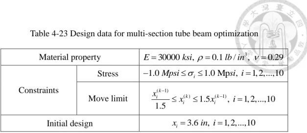
Table 4-23 Design data for multi-section tube beam optimization ... 57

Table 4-24 Result of TAMMA in multi-section tube beam optimization ... 57

Table 4-25 Result comparison for multi-section tube beam optimization ... 58

Table 4-26 Design data for multi-section rectangular beam optimization ... 59

Table 4-27 Result of TAMMA in multi-section rectangular beam optimization ... 60

Table 4-28 Result comparison for multi-section rectangular beam optimization ... 60

Table 5-1 Material properties of gantry structure ... 63

Table 5-2 Design data for self-weight optimization of gantry structure ... 64

Table 5-3 Result of TAMMA in self-weight optimization of gantry structure ... 64

Table 5-4 Result comparison for self-weight optimization of gantry structure ... 65

Table 5-5 Design data for modal optimization of gantry structure ... 66

Table 5-6 Result of TAMMA in modal optimization of gantry structure ... 66

Table 5-7 Result comparison for modal optimization of gantry structure ... 67

Table 5-8 Design data for combinational optimization of gantry structure ... 68

Table 5-9 Result of TAMMA in combinational optimization of gantry structure ... 68

Table 5-10 Result comparison for combinational optimization of gantry structure ... 69

Table 5-11 Material properties of electric scooter ... 70

Table 5-12 Design data for drop test optimization of electric scooter ... 73

Table 5-13 Result of TAMMA in drop test optimization of electric scooter-1 ... 74

Table 5-14 Result of TAMMA in drop test optimization of electric scooter-2 ... 74

Table 5-15 Result comparison for drop test optimization of electric scooter ... 75

Table 5-16 Design data for double drum test optimization of electric scooter ... 78

Table 5-17 Result of TAMMA in double drum test optimization of electric scooter-1 ... 78

Table 5-18 Result of TAMMA in double drum test optimization of electric scooter-2 ... 79

Table 5-19 Result comparison for double drum test optimization of electric scooter ... 79

Table A-1 Necessary files for optimization program ... 86

Table A-2 Necessary files for finite element analysis ... 87

Table A-3 Necessary files for creating CAD model ... 87

Table B-1 Necessary files for sensitivity analysis program ………90

LIST OF SYMBOLS

d Search direction E Young’s modulus e r Relative error

 

f x Objective function value at the test point

 

f x Approximate function value at the test point

 

h x Original function to be approximated

 

h x Function value at the current design point

 

h x Function value at the previous design point

 

h x Approximate function in terms of x

 

h y Approximate function in terms of y n Number of design variables

n b Number of behavior constraints n c Number of constraints

n s Number of size constraints

x 0i i-th design variable at the current design point x 1i i-th design variable at the previous design point

x i i-th design variable x Design variable vector

x 0 Design variable vector of the current design point x 1 Design variable vector of the previous design point

 ^k

xi i-th design variable in k-th iteration

^{k 1}

xi ^ i-th design variable in (k-1)-th iteration

y 0i i-th intervening variable at the current design point y i i-th intervening variable

y Intervening variable vector

y 0 Intervening variable vector of the current design point

 

h x x



 Sensitivity of h x with respect to

 

 

h x x



 Sensitivity of h x with respect to

 

 Step size along the d direction

 Given number

 w Allowable displacement

 Poisson’s ratio

 Density

 i Stress in the i-th element

LIST OF APPROXIMATION METHODS

AQA Adaptive quadratic approximation CONLIN Convex linearization approximation

EMMA Exponential method of moving asymptotes ETPEA Enhanced two-point exponential approximation GBMMA Gradient-based method of moving asymptotes

ISE Incomplete series expansion

ITPA Improved two-point approximation MCA Modified convex approximation MMA Method of moving asymptotes

QTCA Quasi-quadratic two-point conservative approximation

QMMA Quasi-quadratic method of moving asymptotes approximation SACA Self-adjusted convex approximation

SAM Spherical approximation method

TANA Two-point adaptive nonlinearity approximation TANA-1 Two-point adaptive nonlinearity approximation-1 TANA-2 Two-point adaptive nonlinearity approximation-2 TANA-3 Two-point adaptive nonlinearity approximation-3

TDQA Two-point diagonal quadratic approximation TPCA Two-point convex approximation

TPEA Two-point exponential approximation

TPPAA Two-point piecewise adaptive approximation

Chapter 1 Introduction

In this chapter, we introduce the subject of structural optimization. It begins with a brief history of structural optimization and continues with the development of approximation methods. Then, the motivation of this thesis is explained, and the outline of this thesis is presented at the end.

1.1 Introduction to structural optimization

Whether now or in the past, engineers try to use materials as efficiently as possible, for instance, to make structures the lightest while keeping the demanded load capacity.

This is known as structural optimization. Conventionally, searching for more efficient structures is a trial-and-error process which is time-consuming and may not obtain the optimal result. With the development of finite element method, it can be applied to analyze the structural characteristics of products. During the design process, the product would be modified for several times, which means that structural analyses must be executed the same number of times. Obviously, this is not an efficient method.

Nowadays, automated structural design is available with integrating well developed finite element analysis software and optimization theory. It can find the optimum design with less subjective judgement. In order to save the time of design process, the concept of approximation which converts implicit structural functions into explicit ones is introduced. There are two kinds of approximation methods. One is the global approximation method which constructs approximate functions in the whole design space, such as polynomial interpolation, and the other is the local approximation method which is discussed and used in this thesis. Local approximation schemes construct approximate functions by the concept of Taylor series expansion, which is based on the response and the sensitivities in a single design point of the design space. It

transforms the problem with implicit structural behavior into a mathematical problem with explicit functions. However, the approximate mathematical problem is only reliable in the vicinity of the design point at which it is generated. Therefore, to obtain the optimal solution of real problem, it needs to solve sequential approximate sub-problems. Also, each sub-problem takes the optimal solution of last iteration as the initial design. This technique is also known as sequential approximate optimization (SAO).

1.2 Paper review

The history of structural optimization can be traced back to the 1904s. Mitchell derived the theoretical lower bounds of the weight of truss structures with stress constraints [1]. Although it is based on ideal and simple structures, it is still an important inspiration for structural optimization. In 1974, Schmit and Farshi applied approximation concepts to convert structural behaviors into explicit functions of design variables [2]. This method turns time-consuming structural analyses into simple approximate functions, and it greatly reduces the time of structural optimization process.

So far, a lot of local approximation methods have been developed. Among these schemes, the direct linear approximation method, which performs the first-order Taylor series expansion in terms of design variables, is the simplest one. However, most structure characteristics are nonlinear, and therefore this method may not be reliable. In order to approximate structural behavior more accurately, some scholars proposed reciprocal approximation method, which uses the first-order Taylor series expansion in reciprocal variables [3]. Although this method can construct more accurate approximations for simple truss problems with stress and displacement constraints, the

function value tends to infinity when the design variable approach zero that may cause inappropriate approximation. To overcome this problem, Haftka and Shore proposed modified reciprocal approximation method to shift the singular point in reciprocal approximation [4].

In 1979, Starnes and Haftka proposed conservative approximation method, which is also known as convex linearization (COLIN) presented by Fleury and Braibant [5, 6].

This method adopts either direct linear or reciprocal approximation for each design variable according to which approximate function value is estimated higher. It means that this method adopts the more conservative one between direct linear and reciprocal approximation for each design variable. In 1987, Svanberg presented the method of moving asymptotes (MMA), which can be regarded as the generalized form of conservative approximation [7]. This method calculates the moving asymptotes by heuristic rules and utilizes the moving asymptotes to adjust the conservatism of approximations, so that the approximation becomes more adaptive and more efficient.

The efficiency of this method depends on the asymptote locations strongly, and therefore some scholars proposed some methods which utilize the first-order or second-order information to obtain the appropriate moving asymptotes [8, 9].

The above methods have been shown to be successful in a lot of applications, but they are all single-point schemes. Therefore, in order to improve the approximation quality, multi-point information can be used to construct reliable mid-range approximations that are valid in a relatively larger region near the design point. In 1987, Haftka et al. proposed two-point modified reciprocal approximation with a strategy to decide the indeterminate coefficients in modified reciprocal approximation [10].

However, it would fail when the sensitivities of two successive points have the different signs. In 1990, Fadel et al. performed the first-order Taylor series expansion with

exponential intervening variables, called two-point exponential approximation (TPEA) [11]. Although this method can determine the exponent by the sensitivity of the previous design point, it would fail when the sensitivities of two successive points have the different signs. In 1994 and 1995, Wang and Grandhi proposed a series of two-point adaptive nonlinear approximations (TANA) based on TPEA, which enhance TPEA by matching the function value of previous design point [12, 13].

However, the above methods are all monotonic schemes, and therefore are not suitable to approximate non-monotonic structural behaviors. It means that these methods have poor convergence and cannot even converge on certain problems. Hence, some scholars have proposed second-order approximation based on Taylor series expansion to achieve the best compromise between conservativeness and accuracy. In 1994, Snyman and Stander presented spherical approximation method (SAM), which appends a quadratic term to direct linear approximation for correcting the function value of the previous design point [14]. In 1997, Zhang and Fleury proposed modified convex approximation (MCA) based on CONLIN to increase the convexity of approximation [15]. In 1998, Xu and Grandhi proposed two-point adaptive nonlinear approximation-3 (TANA-3), which appends a term to TPEA for matching function value of the previous design point [16]. In 2001, Kim et al. presented two-point diagonal quadratic approximation (TDQA), which adds shifting level into exponential intervening variables to avoid the singularity of the sensitivities in TPEA [17]. In 2007, Groenwold et al. proposed incomplete series expansion (ISE), which includes a series of approximations [18]. ISE uses quadratic, cubic, and even higher order diagonal terms to construct the approximate functions. In 2008, Kim and Choi proposed enhanced two-point diagonal quadratic approximation to reinforce TDQA with new quadratic correction terms by the concept of TANA-3 [19].

In fact, the constraint functions are generally neither purely monotonic nor purely non-monotonic. Therefore, in 1995, Fadel considered the monotonicity of the structural behavior to construct the approximate functions [20]. Then the mixed method named DQA-GMMA is proposed, which adopts monotonic approximation for design variable when the sensitivities of two successive design points have the same signs, and vice versa. Furthermore, several approximation schemes have the approximate function convex to ensure stability of the optimization process, such as GCMMA [21, 22]. In 2015, Li made the approximate functions be strictly convex to improve the robustness and convergence performance of the optimization process, called adaptive quadratic approximation (AQA) [23]. However, this enforcement would cause inconsistency and may lower the efficiency of optimization process.

Moreover, in 2000, Chiou proposed two new convex approximation methods, including self-adjusted convex approximation (SACA) and two-point convex approximation (TPCA) [24]. Both methods are developed based on conservative approximation to achieve numerical stability. In 2002, Chen proposed improved two-point approximation (ITPA), which can be seen as the combination of linear-reciprocal and TPEA [25]. In 2007, Chang proposed quasi-quadratic two-point conservative approximation (QTCA) to improve the conventional conservative approximation methods [26]. In 2010, Chen proposed exponential MMA (EMMA), which makes the order of intervening variables in MMA adjustable for more flexibility [27]. In 2012, Chen proposed a new mixed two-point approximation method, which is the combination of TPEA and GBMMA [28]. When the sensitivities of two successive design points have the same signs, the TPEA scheme is used. Otherwise, the GBMMA scheme is considered. In 2013, Jiang proposed enhanced two-point exponential approximation (ETPEA) that uses intervening variable which is the second order Taylor

series expansion of the original variable to deduce the new formula as the remedy of TPEA [29]. This method can still construct the approximate function when the exponent in TPEA cannot be calculated. In 2016, Wang proposed quasi-quadratic method of moving asymptotes approximation (QMMA), which adds a non-spherical second-order term to MMA to improve the accuracy and efficiency [30]. In the same year, Ke proposed two-point piecewise adaptive approximation (TPPAA), which utilizes the piecewise approximate functions to consider the monotonicity of structural behavior to ensure the quality [31].

1.3 Research motivation

The approximation quality is the crucial factor for the efficiency and stability in SAO process. If the approximate function is accurate, the result can converge in few iterations. On the contrary, it would take more iterations or even diverge. Hence, the use of appropriate approximation is a very important issue in structural optimization design.

Among all the approximation methods, conservative approximations are the most popular methods and widely applied in structural optimization problems. However, the accuracy of these methods are generally considered inadequate. Therefore, in this thesis, in order to deal with this problem, we present a new approximation method named two-point adaptive method of moving asymptotes approximation (TAMMA), which is based on the concept of conservative approximations and derived for considering the monotonicity of structural behavior to construct the approximate functions.

1.4 Outline

In this thesis, there are six chapters, which are briefly described as follows:

Chapter 1: Introduce the development of structural optimization and the existing approximation methods briefly. Also, the research motivation of this thesis is

mentioned.

Chapter 2: Introduce the procedure of mathematical optimization in this thesis and the details on several existing approximation methods.

Chapter 3: Show the derivation of new approximation method developed in this thesis, and the characteristics of the new method is compared with others.

Chapter 4: Apply the proposed new approximation method to several optimization problems of small scale structures, and compare the results with others.

Chapter 5: Apply the proposed new approximation method to several optimization problems of large scale structures, and compare the results with others.

Chapter 6: Provide some conclusions of this thesis and some recommendations for future works.

Chapter 2 Application of approximation methods in structural optimization

In this chapter, we start with an introduction to the procedure of mathematical optimization. Next, several previous approximation methods are discussed, including monotonic, non-monotonic, and considered-monotonicity approximations.

2.1 Mathematical optimization procedure

In this section, we introduce the detailed process of the mathematical optimization in sequence. The general optimization problem can be written as

 

 

Find ,

such that min,

subject to _i 0, 1, 2..., _c, x

F x

g x i n



 

(2.1)

where x denotes the design vector, ^{F x}

 

 

denotes the i-th constraint, and n denotes the number of constraints. _c

2.1.1 Selection of design variables

The parameters that are allowed to change during the design optimization are called design variables. In general, the design variables are continuous and independent in optimization problem. The dimensions of structures, such as cross-section area, height, or thickness, are often chosen as design variables.

Considering efficiency, an optimization problem should avoid having too many design variables. There are two strategies to reduce the design space. One is to choose the dominant variables only instead of all the possible ones, and the other is to link the design variables, which can be written as

 

x T X (2.2)

where X denotes the basis of original design vector, x denotes the reduced basis, and

 

2.1.2 Definition of objective function

A function of the design variables that is to be maximized or minimized is called an objective function. In general, it is often the total weight of structures. In this thesis, the mathematical optimization problem is defined to minimize the objective function as the expression of (2.1). It has no loss of generality since the minimum of the negative objective function occurs where the maximum of objective function happens, which can be written as

       

max F x  min F x , (2.3)

Moreover, in order to treat the problem of multiple objective functions, we can combine each objective function by weighted coefficients. It can be written as

   

1 i i ,

i

F x w F x







where F x denotes the total objective function,

 

 

objective function, and w denotes the weighted coefficient. _i

2.1.3 Treatment of constraints

The design restrictions that must be satisfied in order to produce an acceptable design are called constraints. In general, there are three kinds of constraints in structural optimizations. One is the behavior constraint, such as stress, displacement, or natural frequency, another is the size constraint, and the other is the move limit constraint. In order to make the form of mathematical problem such as (2.1), and avoid the influences of numerical difference between different constraints, the constraints should be modified as follows.

A. Behavior constraint

Stress and displacement constraints are often required in structural optimization to avoid structural breakage or large displacement which influences the performance of structures. These two constraints can be written as

, 1, 2,..., , 0, 0,

L U

i i i b

L U

i i

g g g i n

g g

  

  (2.5)

where g_i^L and g^U_i denote the lower and upper bound of the i-th constraint, and n _b denotes the number of behavior constraints.The constraints should be modified as

1.0, if 0

1, 2,..., , 1.0, if 0

i U i M i

i b

i L i i

g g

g g i n

g g

g

  

 

  



(2.6)

where g_i^M denotes the modified constraints.

Furthermore, we may want to change the natural frequencies of a structural object, so as to avoid resonance with other parts in design. Increasing the natural frequencies is the general strategy, and therefore the natural frequencies of the structure are often restricted in certain region. The constraints can be written as

, 1, 2,..., , 0.

L

i i b

L i

g g i n

g

 

 (2.7)

The constraints should be modified as

1.0 , 1, 2,..., .

M i

i L b

i

g g i n

 g  (2.8)

B. Size constraint

Size constraints are the limits of design variables due to material specifications, practical demands, and so on. Size constraints can be written as

, 1, 2,..., ,

L U

i i i s

D  x D i n (2.9)

where D_i^L and D_i^U denote the lower and upper bounds of allowable sizes, and n _s denotes the number of size constraints.

C. Move limit

In the local approximation, approximation is trustable only around the current design point. Therefore, some artificial constraints of design variables which called move limit must be added to the optimization problem. It can be written as

, 1, 2,..., ,

L U

i i i

x x x i n

      (2.10)

where x_i^L and x^U_i denote lower and upper bound of the variations of the i-th design variable, and n denotes the number of design variables.

2.1.4 Application of approximation methods

As long as the mathematical problem is defined, the optimal solution can be found by mathematical programming. However, the relation between structural behavior and design variables is usually implicit. That is why the approximation technique which convert the implicit behavior into explicit functions is applied. Local approximations are only reliable in the vicinity of the design point at which they are generated because the approximate functions are variations on the Taylor series expansion. Therefore, we cannot obtain the optimal solution of mathematical problem for one time. If the current optimal solution is not satisfactory, the approximations of the objective and constraint functions need to be modified by the current optimal solution, and then the approximate problem is solved again. Repeat this step until the convergence criteria are satisfied.

This gradual improvement process is known as sequential approximate optimization (SAO).

2.1.5 Application of sensitivity analysis

Most local approximation methods adopt Taylor series expansion to construct the

approximate function. In these methods, it is necessary to calculate the derivatives of behavior functions with respect to design variables, which are called sensitivities. This is an essential step in approximations, called sensitivity analysis.

Sensitivity analysis is the way to realize the variation tendency of structural behavior with respect to design variables. In this thesis, backward difference method is adopted in sensitivity analysis, which can be written as

0 0 0

( ) ( ) ( )

i ,

i i

h x h x h x x

x x

   

   (2.11)

where h x

 

i i

x x

   represents that only the i-th design variable has a small variation  . Moreover, x_i  can be written as x_i

0 ,

i i

x  x

   (2.12)

where  is an extremely small number with respect to x . _0i

2.1.6 Application of mathematical optimization

Mathematical optimization method can be classified into direct and indirect methods. Direct method is to solve the optimization problems without transferring the constraints, such as the method of feasible direction. As for indirect method, it converts the constraints to a part of objective function, hence the constrained problems can be transferred to unconstrained problems, such as interior penalty method and exterior penalty method.

Most methods demand a feasible starting point to solve constrained optimization problems, such as feasible direction and interior penalty methods. However, it cannot guarantee that the initial design is always in the feasible domain in iterative process.

Therefore, exterior penalty method which make the process valid with infeasible initial

design is adopted to deal with the constrained problems in this thesis. After transformation, the objective function can be written as

2 1

( , ) ( ) ( ) ,

( ), if ( ) 0 ( ) 0, if ( ) 0,

nc

i i

i i

i

i

x r F x r g x

g x g x

g x g x



    

 

   



(2.13)

where ( , )x r denotes the penalized objective function, F x( ) denotes the objective function, r denotes the penalty factor, and g x denotes the i-th constraint function. _i( )

2.2 Monotonic approximation methods

The approximation methods described in this section have been shown to be successful in a lot of applications, but they are all first-order Taylor series expansion and monotonic schemes. Therefore, they are not suitable to approximate non-monotonic structural behaviors.

2.2.1 Direct linear approximation

The direct linear approximation method is the most fundamental and simplest one in approximation method. If h x( ) denotes the function to be approximated, this approximation can be written as

 

0 0

1

( ) ( ) ( ),

n

l i i

i i

h x h x h x x x

 x

   



where h x denotes the direct linear approximate function of _l( ) h x( ), and x denotes ₀ the variable vector of current point with i-th component x . _0i

However, this method is often unreliable because most behavior functions of general structures are nonlinear.

2.2.2 Reciprocal approximation

In structural optimization problems, sizing parameters such as cross-section area of

beams and thickness of plates are often chosen as design variables, and structural characteristics such as stress and displacement are often chosen as constraints. In this kind of problem, the relation between the reciprocals of design variables and structural behavior functions are often near linear. Hence, in this case, using the first-order Taylor series expansion in reciprocal design variables yields the better approximation in comparison with the direct linear approximation, which is called reciprocal approximation method [3]. This approximation can be written as

 

0 0

1

( ) ( ) ( )( ),

n

i

r i i

i i i

h x x

h x h x x x

x x



   



where h x denotes the reciprocal approximate function of _r( ) h x( ).

However, x _i 0 is the singular point in this approximation method. When the design variable approaches to the singular point, the magnitude of the function value and sensitivity tends to infinity. Therefore, the approximation quality would be affected.

2.2.3 Modified reciprocal approximation

In order to rectify the defect of reciprocal approximation method, the modified reciprocal approximation method shifts the singular point to expand the reliable region [4]. This approximation can be written as

 

0 0

1

( ) ( ) ( )( ),

n

i mi

mr i i

i i i mi

h x x x

h x h x x x

x x x



 

  

 



where h_mr( )x denotes the modified reciprocal approximate function of h x( ). The singular point is shifted from zero to x_mi, but the magnitude of x needs to be _mi determined by experience.

2.2.4 Conservative and convex linearization approximation

This is a type of mix approximation which combines the direct linear and

reciprocal approximation methods, called conservative approximation method or convex linearization method (CONLIN) [5, 6].This approximation can be written as

 

 

0 0 0

1 1

( ) ( ) ( ) ( ) ⁱ ,

c i i i i

i i i i i

h x h x x

h x h x x x x x

x x x

 

 

   

 





where h x denotes the CONLIN approximate function of _c( ) h x( ),

1 i





1 i





the summation of the design variable with negative first-order sensitivity.

This method can estimate larger function values compared with the direct linear and reciprocal methods, which means that the function values of behavior constraints are estimated conservatively. Of course, conservativeness is an important factor for approximation methods. But the too conservative approximation would reduce the convergence rate and result in low efficiency to the optimization process.

2.2.5 Method of moving asymptotes

The CONLIN uses a combination of direct linear and reciprocal approximation, and there is no direct control on the convexity of the approximation. The method of moving asymptotes (MMA) adjusts the convexity of CONLIN approximation by adding two sets of new parameters, the upper and lower asymptotes, U and _i L [7]. Either _i 1/ (U_ix_i) or 1/ (x_iL_i) is used in the first-order Taylor series expansion, depending upon the signs of the first-order sensitivities with respect to the design variables. This approximation can be written as

0 2

0 0

=1 0

0 2 0

=1 0

( ) 1 1

( ) ( ) ( )

( ) 1 1

( ) ,

mma i i

i i i i i i

i i

i i i i i i

h x h x h x U x

x U x U x

h x x L

x x L x L





 

        

 

       





(2.18)

where h_mma( )x denotes the MMA approximate function of h x( ).

In this method, there are three strategies to calculate the artificial upper and lower bounds [7-9].One is to use heuristic rules, which can be written as

 

 

0 1 1

0 1 1

, ,

i i i i

i i i i

U x s U x

L x s x L

  

   (2.19)

where x denotes the i-th component of the previous design point vector _1i x , ₁ U and _1i

L denote the asymptotes in the previous iteration, and 1i s denotes the positive scalar parameter. Another is to use the information of the second-order sensitivity, which can be written as

2

0 0

0 2

( ) ( )

, 2 .

i

i i i

i

h x h x

U L x

x x

 

 

  (2.20)

And the other is to use the information of the first-order sensitivity, which can be written as

   

     

0 1

0 1

0

0 1 0 1

0

, if 0

, 1

2 , if 0,

1

i i

i

i i

i

i i

i i i

i

i i i

h x h x x x

x x x

U L

x x h x h x

x x x







 

    

   

 

  

   

   



(2.21)

where _i ^{( )0 ( )1} .

i i

h x h x

x x

  ^{ }

 

Moreover, based on (2.18), if U   and _i L  , MMA is reduced to CONLIN _i 0 and to direct linear approximation if further L   . Therefore, the direct linear and _i CONLIN can be regarded as the special cases of MMA.

2.2.6 Two-point modified reciprocal approximation

The two-point modified reciprocal approximation method utilizes the information of two successive design points to determine the indeterminate coefficient in modified

reciprocal approximation method [10]. Its mathematical form is the same as (2.16), but x is determined by fitting the sensitivity of the previous design point, which can be mi

derived as

 

 

0 1

, .

1

i i i

mi i

i i

i

h x h x

x x

x x x

 



 

  

 

 (2.22)

Obviously, it would fail when the two derivatives have the different signs.

Moreover, x is required to be a positive number to avoid the function value tending _mi infinity, but it is not guaranteed in this method.

2.2.7 Two-point exponential approximation

To control the curvature of reciprocal approximation and make it more adaptive, the two-point exponential approximation method (TPEA) takes x_i^pi as the intervening variable for the first-order Taylor series expansion [11]. This approximation can be written as

   

 





1

,

i

i i

n p

p p

i

tpea i i

i i i

h x x

h x h x x x

x p





   



where h_tpea( )x denotes the TPEA approximate function of h x( ). p is determined by _i fitting the sensitivity of the previous design point, and it can be derived as

   

 

1 0

1 0

ln

1 .

ln

i i

i

i i

h x h x

x x

p x x

 

 

   

 

  (2.24)

However, this calculation would fail in following two conditions:

 

 

1 0

0 or _{i i} 0.

i i

h x h x

x x

x x

 

 

  (2.25)

When p cannot be calculated by matching the sensitivity, the author suggests _i substituting p with 1. Moreover, to avoid inappropriate approximation, _i p should be _i

restricted between p and ^L p .^U Also, p   and ^L 1 p  is suggested by the ^U 1 author. When p is smaller than _i p with calculated from (2.24), ^L p_i  p^L is adopted, and vice versa.

Based on (2.23), if p  , TPEA is reduced to direct linear approximation, and if _i 1

i 1

p   , it is reduced to reciprocal one. Therefore, the direct linear and reciprocal approximations can be regarded as the special cases of TPEA.

2.2.8 Two-point adaptive nonlinearity approximation

The two-point adaptive nonlinearity approximation (TANA) takes x_i^r as the intervening variable for the first-order Taylor series expansion [12]. In this method, the concept is similar to TPEA, but the orders of design variables are the same within approximate functions. This approximation can be written as

     

 

tana 0 0

1

,

n r

r r

i

i i

i i

h x x

h x h x x x

x r





   



where h_tana( )x denotes the TANA approximate function of h x( ). r is determined by fitting the function value of previous design point, and (2.26) can be rewritten as

 

 

 





1

.

n r

r r

i

i i

i i

h x x

h x h x x x

x r





   



However, the above formula is a nonlinear equation of r. Therefore, in order to solve this equation, the utilization of numerical methods is necessary. The drawback of TANA is that it may have no solution for (2.27).

2.2.9 Two-point adaptive nonlinearity approximation-1

In order to build the high quality approximations to realize computational savings in solving complex optimization problems, the two-point adaptive nonlinearity approximation-1 (TANA-1) based on TPEA takes expansion at previous design point

and adds a correction term  to simulate the higher order terms of the Taylor series ₁ expansion [13]. This approximation can be written as

     

 

tana1 1 1 1

1

,

i

i i

n p

p p

i

i i

i i i

h x x

h x h x x x

x p^ 



    



where h_tana1( )x denotes the TANA-1 approximate function of h x( ). p is determined _i by fitting the sensitivity of the current design point, and it can be derived as

   

 

0 1

0 1

ln

1 .

ln

i i

i

i i

h x h x

x x

p x x

 

 

   

 

  (2.29)

Then,  is determined by fitting the function value of the current design point, which ₁ can be derived as

     

 

1 0 1 0 1

1

.

i

i i

n p

p p

i

i i

i i i

h x x

h x h x x x

x p

 ^



    



In this method, it has the similar drawback with TPEA that is the value of p _i

cannot be calculated when

 

 

0

i i

h x h x

x x

 

   or x_0i x  . _1i 0

2.3 Non-monotonic approximation methods

The concept of adding second-order terms to the monotonic approximation has been applied to increase the accuracy of the approximations in many approximation methods, and it make the approximation non-monotonic. Some of the important non-monotonic approximations are presented in the following section.

2.3.1 Spherical approximation method

The spherical approximation method (SAM) adds an approximate quadratic term to the direct linear approximation method to increase the accuracy of the approximations [14]. This approximation can be written as