適用於相同多核心系統的測試壓縮及診斷機制之LZSS壓縮演算法及硬體架構設計

(1)

國立臺灣大學電機資訊學院電子工程學研究所碩士論文

Graduate Institute of Electronics Engineering College of Electrical Engineering & Computer Science

National Taiwan University Master Thesis

適用於相同多核心系統的測試壓縮及診斷機制之 LZSS 壓縮演算法及硬體架構設計

LZSS Compression Algorithm and Architecture for Test Compression and Diagnosis of Identical Multicore Systems

曾煥富

HUAN-FU ZENG

指導教授：吳安宇博士 Advisor: AN-YEU WU, Ph.D.

(2)

(3)

(4)

(5)

致謝

經過了數不清的無力感，歷經了無數的情緒起伏，我終於走向了碩士訓練最後的一關。首先我要感謝吳安宇教授的指導。從大學部專題到研究所，漫長的五年半，您總是非常有耐心地指導著我。您投注在我身上的心血，以及對我的勉勵和關照，令我永生難忘。也感謝口試委員們：李建模教授和陳坤志教授，以及來幫我預口試的黃俊郎教授，給我非常寶貴的意見及指導。

在Access IC Lab 這片沃土中，有汗水、有笑聲。在此我孕育著我的夢想，

厚植著我的研究能力。從賢楷、恩瑞、坤志、Foster 學長，到 Woody、Darcy...，

以及各位同學、學弟妹們，實驗室是凝聚我們的生命共同體。我想特別感謝林祐民學長：從我碩二以來的幫忙，與我一同面對我的困難，給我非常多的協助、信心。

同時，我也要感謝台大領袖社的夥伴們，我們一起奮鬥的辛酸血淚。有你們在，我艱辛的研究路上多了陪伴。在研究所的訓練中，我慢慢地認識自我，補足我從小以來一直非常欠缺的人際關係。也是因為吳老師的愛與包容，讓我終於走出了一條自己的道路。

祝福還在Lab 的各位同學、學弟妹們，都能夠順利畢業，以 Access IC Lab

的訓練，在各界大展身手。最後，將深深的愛與祝福，獻給我的家人、家族。

曾煥富謹誌 105 年 7 月 26 日

(6)

摘要

目前隨著多核心 CPU 及 GPU(圖形處理單元)的普及，且核心數量由多核轉為眾核，測試資料急速的增加。然而由於自動測試機的傳輸頻寬及接腳數目有限，相較於測試資料的增加並未顯著上升，因此造成測試時間的上升，也就是測試成本的提升。為了達到降低測試成本，測試壓縮被廣泛地採用。

測試壓縮可分為測試激勵壓縮(test stimulus compression)及測試響應壓縮 (test response compaction)。測試激勵壓縮是指在經由自動測試圖樣產生(ATPG) 測試資料後，將測試資料做無損壓縮，並存於自動測試機(ATE)。當進行測試時，

由自動測試機讀取測試資料傳輸至待測電路，並經過待測電路上之解壓縮器解壓，

再進行測試。測試響應壓縮則是在待測經過測試後，將測試響應做壓縮，傳回自動測試機。在經過測試後，若有錯誤，可由診斷機制判斷錯誤發生之原因。

傳統相同多核心測試響應壓縮，使用有損壓縮方式，以達成高壓縮倍率。然而，

這會使診斷進行變得困難。為保留完整測試響應資訊，本論文採用無損的 LZSS 壓縮演算法。由於無損的特性，可使測試響應壓縮之後，可以保留完整的響應資訊，

以利後續的診斷。

在硬體實現方面，我們設計一高速之 LZSS 解碼器硬體架構，作為晶片內測試激勵壓縮之解壓縮器。同時我們設計一高速、可規模化的 LZSS 編碼器硬體架構，

作為晶片內部測試響應壓縮之壓縮器。本論文提出適用於相同多核心，基於 LZSS 的無損測試壓縮機制，可以達到高速、可規模化，且可支援診斷機制之測試壓縮系統。

關鍵字：測試激勵壓縮、測試響應壓縮、診斷、相同多核心、LZSS、演算法、可規

(7)

(8)

Abstract

As the current multi-core CPU and GPU prevail, and the core number increases from multi-core to many-core, the test data increases rapidly. Due to the limited transmission bandwidth and pin counts of the automatic test equipment (ATE), test time as well as test cost rise. In order to lower test costs, test compression is widely adopted.

Test compression can be divided into test stimulus compression as well as test response compaction. Test stimulus compression refers to the fact that, after the test data is generated using automatic test pattern generation (ATPG), it is compressed and stored in the memory of the ATE. During test, the test data is read out from the ATE memory and decompressed on chip before sending into the design-under-test (DUT). Test response compaction, on the other hand, refers to the fact that after the design under test is tested, the test response data is compressed on-chip and sent back to the ATE. After the test response compaction, we can further analyze the test response to do circuit diagnosis, which refers to finding out the fault that causes the output error.

(9)

Conventional test response compaction uses lossy compression in order to reach high compressibility. However, it is difficult to diagnose the circuit fault using the compacted test response. In order to better diagnose the circuit, we use lossless compression algorithm, LZSS, to do the test response compaction. Therefore, the full test response information can be utilized to do better circuit diagnosis.

This thesis proposes a lossless test compression scheme for identical multicore systems using LZSS compression algorithm. The broadcast-based test stimulus compression does not differ from the single core case much; thus, we focus on the algorithm design for test response compaction. Owing to the lossless compression capability of the LZSS algorithm, test response information is fully sustained after the test response compaction, which can be better utilized in the circuit diagnosis. In the hardware aspect, we first design a high-throughput LZSS-based decoder for test stimulus decompression on-chip. Second, we design a high-speed and scalable LZSS-based encoder for test response compaction on-chip.

(10)

List of Figures

Figure 1.1 Typical IC manufacturing flow [1]... 2 Figure 1.2 Example of multi-core CPU and GPU: (a) Intel Single Chip Cloud Computer 48 cores [10]. (b) Intel Tera-flops Research Chip 80 cores [9]. (c) Nvidia GeForce GTX 980 (2048 cores) [5]. ... 2 Figure 1.3 The test data amount grows dramatically with the circuit size [4]. ... 3 Figure 1.4 Test compression reduces the amount of test data transmitted from the automatic test equipment (ATE) and back [1]. ... 4 Figure 1.5 The flow of test pattern generation, including test stimulus compression and test response compaction. ... 4 Figure 1.6 Test compression for identical multiple cores. ... 7 Figure 1.7 The proposed on-chip test stimulus decompressor and the test response compactor system with the design-under-test (DUT) shown. ... 9 Figure 2.1 The system architecture of related work [6]: (a) Full system architecture and (b) An example of 3-input majority analyzer (MA). ... 14

(14)

Figure 2.4 Three different combinations of scan cells result in three different partition circuits: (a) the first partition circuit, and (b) adding the second partition circuit, and (c) adding the third partition circuit. ... 17 Figure 2.5 Compaction scheme for diagnosis. ... 17 Figure 3.1 Two possible compaction schemes: (a) compress different scan chains in the same core vs. (b) compress the respective same chains between different cores. .. 21 Figure 3.2 Pseudocode for LZSS compression algorithm. ... 23 Figure 3.3 The LZSS encoding algorithm. ... 25 Figure 3.4 Experiment result demonstrating the LZSS compressibility. ... 26 Figure 3.5 Proportion of don’t-care bits in 200 test stimulus patterns of the s38417 benchmark circuit ... 29 Figure 3.6 Naïve don’t-care bits assignment using adjacency filling. ... 30 Figure 3.7 Experiment of test stimulus compression: fill the test stimulus don’t-care bits using adjacency filling. ... 31 Figure 3.8 The multicore error probability of each individual core pi can be modeled as i.i.d. exponential random variables with mean λi. ... 32 Figure 3.9 The histogram of core error probability in this experiment. ... 33 Figure 3.10 The formation of an LZSS symbol for test response compaction. ... 33

(15)

Figure 3.11 The histogram of compression ratio result of 100 test patterns, each with

length of 1024 bits. ... 34

Figure 3.12 The compression ratio versus the error rate parameter λ and core count N. 35 Figure 3.13 The compression ratio result as LA_BF and SW varies. ... 37

Figure 4.1 Hardware architecture for LZSS decoder. ... 41

Figure 4.2 The finite state machine (FSM) of the decoder. ... 41

Figure 4.3 The timing diagram of LZSS decoder. ... 41

Figure 4.4 Symbol combining for shared mux control input. ... 42

Figure 4.5 The chip layout of LZSS decoder design core. ... 44

Figure 4.6 Content addressable memory (CAM): (a) The whole CAM architecture and (b) a cell of the CAM. ... 45

Figure 4.7 Systolic-array-based LZSS encoder: (a) the systolic array architecture; (b) the space-time diagram of (a); (c) the processor element of each circle of (a). ... 47

Figure 4.8 Block diagram of LZSS encoder architecture. ... 49

Figure 4.9 (a)-(d) A case study of the encoding process. ... 52

(16)

Figure 4.13 Parallel comparators of Figure 4.11 and Figure 4.12. ... 55 Figure 4.14 The 4-unfolded parallel comparison logic for the sliding window. ... 56 Figure 4.15 (a) The pipelined maximum selection tree with two comparator stages in one pipeline stage, and (b) the structure of each node in (a). ... 57 Figure 4.16 The codeword formation example. ... 58 Figure 4.17 (a)(b) The processing element and the best-match encoder. ... 59 Figure 4.18 Proportions of the area in the 4-unfolded LZSS encoder architecture. .... 60 Figure 4.19 The encoder design is scalable as the core number grows. ... 60 Figure 4.20 The chip layout of LZSS encoder design core. ... 61

(17)

List of Tables

Table 2.1 Comparison between related works and proposed approach. ... 18

Table 3.1 The codeword types of LZSS encoding algorithm. ... 24

Table 3.2 The compression gain at certain representation ... 26

Table 3.3 Simulation setting of test stimulus compression. ... 31

Table 3.4 The settings of Experiment 1. ... 35

Table 3.5 The settings of experiment 2. ... 37

Table 4.1 Synthesis result of LZSS decoder. ... 44

Table 4.2 The implementation result of LZSS decoder. ... 45

Table 4.3 Synthesis result of the 4-unfold LZSS encoder. ... 58

Table 4.4 The implementation result of LZSS encoder. ... 62

(18)

Chapter 1 Introduction

1.1 VLSI Testing and Test Compression

1.1.1 VLSI Testing

Testing of very-large scale integrated (VLSI) circuits plays an important role in the process of chip production, as shown in Figure 1.1. After the chips designed by the designers are fabricated, they need to go through a couple of tests to ensure the correctness of their functionality. As there are more and more transistors in the current VLSI circuits, and as the process goes deep-submicron, there are more defects on chip.

We often model the defects as circuit faults, for example, stuck-at faults and transition delay faults, and we generate test patterns to test these circuit faults. As modern CPU and GPU prevail and go towards many-core era (Figure 1.2), the test data also increases nearly exponentially with time [4], as shown in Figure 1.3, making testing of chips a challenge. Therefore, we need a good way to reduce the amount of test data.

(19)

Figure 1.1 Typical IC manufacturing flow [1].

(a) (b)

(c)

(20)

Figure 1.3 The test data amount grows dramatically with the circuit size [4].

In the current VLSI test scenario, the test patterns are stored in the automatic test equipment (ATE). The limited pin count and limited bandwidth compared with the amount of test data makes test time as well as test cost large. The technique of reducing the amount of test data transmitted from the automatic test equipment (ATE) to the design-under-test (DUT) and back during circuit test is called test compression. We can use test compression usually reduce the amount of time spent and also reduce the test bandwidth requirement.

(21)

Figure 1.4 Test compression reduces the amount of test data transmitted from the automatic test equipment (ATE) and back [1].

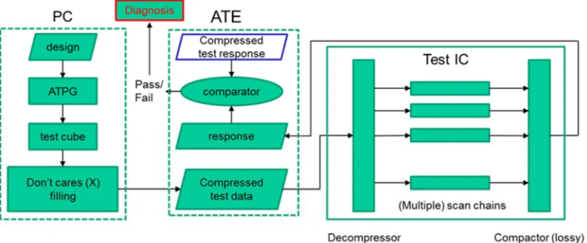
Figure 1.5 The flow of test pattern generation, including test stimulus compression and test response compaction.

(22)

1.1.2 Test Flow and Test Compression

Test compression can be divided into two categories: one is the test stimulus compression, and the other is the test response compaction. The way to reduce the test stimulus data transmitted from the ATE to the core is called test stimulus compression, and the way to reduce the test response data transmitted from the core back to the ATE is called test response compaction.

The full test flow is shown in Figure 1.5. The test stimulus is generated via the automatic test pattern generation (ATPG) process. The test stimulus data, or the test vector (we would use these two terms interchangeably), generated by the ATPG process contains many don’t-care bits (X’s) that can be filled with either 1 or 0. We need to fill the don’t-care bits before the test patterns are applied to the DUT. We can fill the test patterns so that patterns are more compressible.

(23)

After the don’t-care bits in the test stimulus data are filled, the test stimulus data will go through test stimulus compression off-line. Test stimulus compression should be done using lossless compression, and therefore the test stimulus data can be recovered using decompressor on-chip. After the test stimulus compression process, we store the compressed test stimulus data on the ATE. When the ATE runs, it sends the compressed test stimulus data on chip and then be decompressed. After the on-chip decompressor decompresses the test stimulus data, they are sent into the scan chains.

As shown in Figure 1.5, before the test response information is sent out of the chip, it needs to go through the test response compactor. Test response compaction is usually lossy. It’s because if we only want to know whether the chip is correct or not, we may simply map the test response to syndrome to see whether the syndrome is equal to the golden syndrome. Using lossy test response compaction can also reduces the compression ratio.

(24)

Figure 1.6 Test compression for identical multiple cores.

The drawback of lossy test response compaction are two: the aliasing problem, and the difficulty to diagnose. The aliasing problem is that, after mapping to the syndrome, if the faulty syndrome is also equal to the golden syndrome, then we misjudge the faulty response to be correct. The difficulty to diagnose refers to the fact that, because the compaction is lossy, we cannot recover the original test response from the syndrome. Therefore, we cannot accurately diagnose the reason of the faulty response.

1.1.3 Identical Multicore Test Compression System

As the trend towards multi-core and many-core systems, such as multi-core CPU [10][11] and GPU [5], testing of these design also raises new problems. The test stimulus compression does not differ from that of single core much, because we can use the same test vector, and broadcast to every core. The test response compaction is more challenging, especially when the core number grows. Because the test response

(25)

of these identical cores may differ from one another, the compaction will also be different from the single core case. We need to design the compactor properly to reach test needs.

1.2 Motivation and Goal

1.2.1 Problem Formulation

Traditionally, diagnosis is done off-line, and we can only know whether the circuit is good or faulty. In the multi-core system, the system may be reused even if some cores are faulty. If we know the correctness of each individual core using circuit diagnosis, we can reuse the functional cores in the system, and reduce the cost of throwing partially faulty chips away.

There are two main problems:

 Test response compaction process is lossy, and test response information cannot be recovered for diagnosis, and

 The test response compactor hardware is not a scalable design when the number of cores of design-under-test (DUT) grows.

(26)

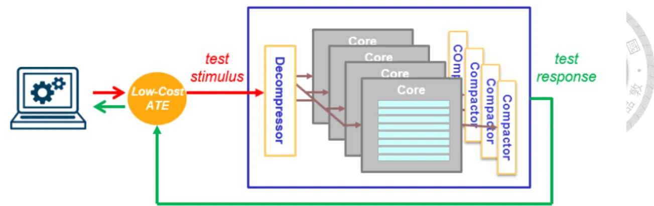
Figure 1.7 The proposed on-chip test stimulus decompressor and the test response compactor system with the design-under-test (DUT) shown.

1.2.2 The Proposed Test Response Compaction Scheme

The proposed test stimulus compression method using lossless compression can be applied to arbitrary test patterns without structural dependency. In the proposed method, we can obtain the exact information of the faulty response of every core.

Furthermore, after diagnosis, the faulty multi-core platform may be reused or recycled to reduce the cost of throwing it away.

The hardware overhead of the proposed method does not increase the test compression hardware complexity too much, and is a scalable method because the system complexity grows slowly as the number of cores scale up, as shown in later sections (Figure 4.19).

(27)

1.2.3 Thesis Goal

We propose a novel test compression scheme for VLSI testing with both test stimulus compression as well as test response compaction, as shown in Figure 1.7. We implement the test stimulus decompressor and the test response compactor on-chip.

 The proposed test stimulus compression may achieve a better compression ratio under the same level of fault coverage (FC), and

 The test response compactor is lossless, and therefore information can be recovered during diagnosis.

The bit width of the on-chip decompressed symbol equals the number of scan chains in every identical core. There are a number of test response compactors in the test response compaction, which also equals to the number of identical cores. The bit width of the compactor symbol is equal to the number of scan chains in the design. All is shown in Figure 1.7 above. The scalability of the compactor as the size of the design- under-test (DUT) grows is described in Figure 4.19.

(28)

1.3 Thesis Organization

The thesis consists of five chapters. Chapter 2 reviews the related work of test stimulus compression and test response compaction. Chapter 3 introduces the LZSS compression algorithm used in test stimulus compression and test response compaction.

Chapter 4 presents the hardware design of the decompressor for on-chip test stimulus decompression as well as the compressor for on-chip test response compactor. Finally, Chapter 5 entails the conclusion and future work.

(29)

Chapter 2 Review of Test Response Compaction Techniques

2.1 Related Works

2.1.1 Majority-Based Test Access Mechanism for Parallel

Testing of Multiple Identical Cores

There are several works related to the test compression of identical multicore systems. In [6], the authors proposes a test access mechanism (TAM) for identical multicore systems, as shown in Figure 2.1(a). They assume that the majority value of the outcomes of all cores are always correct, and therefore use them as golden responses.

In test response compaction, all scan chains in every single core are compared (XORed) with the majority values respectively. After the XOR stage, the values are ORed

(30)

However, the method suffers from two problems. Although we can deduce from the faulty response the correctness of the core, we have a hard time to know the exact fault location. That is, we cannot diagnose the circuit. The author in [6] proposes a method to refeed the scan chain and do the fault simulation again, and go through different paths to do the diagnosis. It may not be acceptable because this doubles the test time as well as test cost.

The method of [6] has two drawbacks: the first being its non-scalable complexity.

The more cores, the larger the majority analyzer (MA) is, and the hardware overhead grows superlinearly. The second is that the diagnosis needs two phases. It first generate the comparison result. If the outcome is all correct, then we are done. However, if the outcome is different from the majority value, then we needs to set MA_sel in Figure 2.1(b) to select the output of the faulty core, and using the flip-flops shown in Figure 2.2 to get the original uncompacted test response.

(31)

(a)

(b)

Figure 2.1 The system architecture of related work [6]: (a) Full system architecture and (b) An example of 3-input majority analyzer (MA).

(32)

2.1.2 A Novel Test Access Mechanism for Failure Diagnosis of

Multiple Isolated Identical Cores

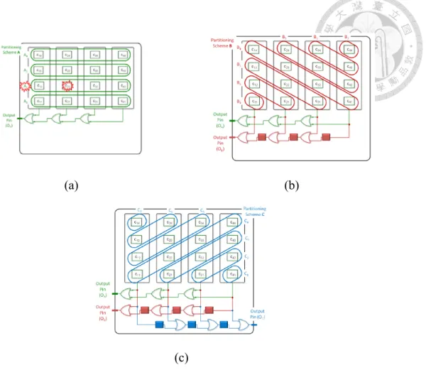
The method of [9] also resembles that of [6]. The difference is that, first, there are separate pins for golden response input in [9]. Second, as for the OR tree, the circuit is grouped into different sets of partitions, as shown in Figure 2.4, which means different ways to do test response compaction. In [9], every “partition” is the OR combination in the partition in every circle. The circle means a combination (e.g. OR), of all the values in the circle, which are the difference bits.

Figure 2.3 The system architecture of related work [9].

(33)

The compaction process goes as follows. In each output pin of each partition, if the OR result is 0, which means all the input pins of the OR gate are 0, the respective scan chains are fault-free. On the contrary, if the OR result is 1, which means all the input pins of the OR gate are not 0, at least one of the scan chains is faulty. When we need to do circuit diagnosis, we can first collect the compacted test response data from different compaction partitions. As shown in Figure 2.5, the circle shown are the test response with value 1, which means error output. To diagnose for the exact position of the faults, we infer from the faulty test response. Cells shown in red background are diagnosed with fault; however, the cell in yellow background cannot be diagnosed whether correct or faulty. Also, the hardware overhead is non-scalable because it needs more sets of “partitions” to generate the “equations” when the circuit grows large.

(34)

(a) (b)

(c)

Figure 2.4 Three different combinations of scan cells result in three different partition circuits: (a) the first partition circuit, and (b) adding the second partition circuit, and

(c) adding the third partition circuit.

Figure 2.5 Compaction scheme for diagnosis.

(35)

2.2 Problems of Related Works

In [6], the test response compaction is lossy. Therefore, we cannot obtain the exact test response for diagnosis. In the identical multicore systems, the diagnosis for each core is even more difficult, because we cannot obtain the exact result of each core. Also, there is test escape due to the aliasing problem of the compacted syndrome.

The underlying reason is that they compress in the same core between different scan chains rather than the same scan chain in respective cores. It does not utilize the information redundancy, and therefore lower the compressibility. The scalability of both methods is not enough, which means as the number of cores grows, the hardware area overhead of the compactor grows superlinearly.

Table 2.1 Comparison between related works and proposed approach.

(36)

2.3 Summary

The architecture of related works [6] and [9] are both non-scalable. [6] uses a majority analyzer, which grows at least as fast as the number of cores grows. [9] uses multiple compaction, and we need more sets of compactors as the scan chain and core number grows. Also, the test response information is hard to recover, which makes diagnosis after compaction impossible. If we can get full test response information, we can improve diagnosis.

(37)

Chapter 3 LZSS-Based Test Compression for Identical Multiple Core Systems

3.1 System Description

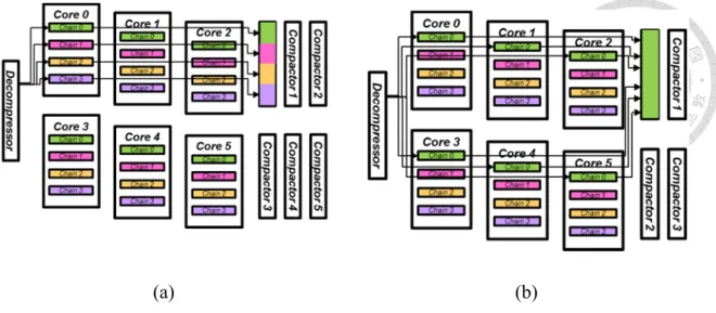
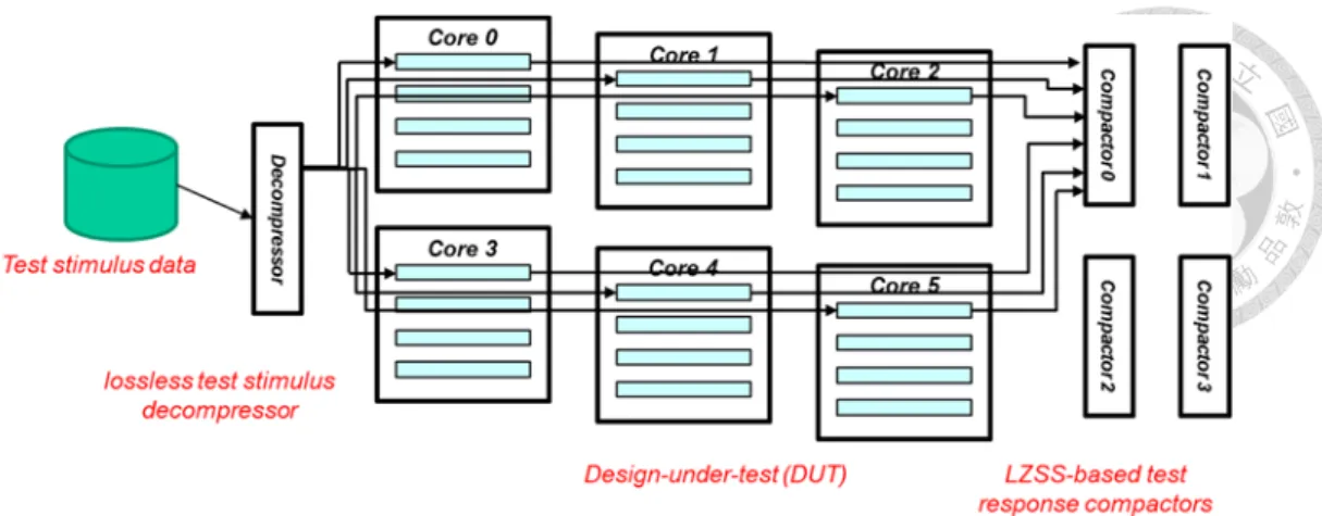
Traditionally, test response compaction are categorized as space compaction and time compaction. Space compaction refers to compacting data in the space dimension, while time compaction refers to compacting data in the time dimension. [1] However, in the identical multiple core systems, there are three dimensions in multicore test response data: core, space (scan chain) and time, where the core dimension is the additional third dimension. We would like to exploit the third data dimension. As shown in Figure 3.1, there are two options. Figure 3.1(a) shows that, if we compress all the scan chains in the same core, just as the configuration described in Chapter 2, the correlation between the data of different scan chains will be low. It results in poor

(38)

(a) (b)

Figure 3.1 Two possible compaction schemes: (a) compress different scan chains in the same core vs. (b) compress the respective same chains between different cores.

3.2 LZSS Compression Algorithms

3.2.1 Introduction to the Algorithm

There are some lossless compression algorithms: Huffman code, arithmetic code, LZ-based compression algorithms, etc. These compression algorithms share the common property of being able to recover the information totally when doing decompression. However, the Huffman code requires additional information of symbol probability distribution, in order to do near-optimal coding of the information. This requires that, before a data stream is compressed, we need to scan through the whole data stream going to be compressed and extract the symbol probability distribution.

Also, constructing the Huffman code requires a binary tree data structure, which causes

(39)

high hardware complexity. Arithmetic code also suffers from the need of preprocessing to get the symbol distribution.

Dictionary-based coding, such as LZ-based compression algorithms and its variants [13][21], are widely used in file compression software and unix system utility.

There are kinds of dictionaries, some are static while others are dynamic (or adaptive).

Using the dictionary, the algorithm replaces the repeating sequence with a shorter code.

The LZSS algorithm belongs to the LZ-based compression algorithm, and is similar to the LZ1, or say LZ77 algorithm, where the pointer to the referenced sequence and the match length is encoded.

The LZSS algorithm is one of the algorithms in the LZ-based compression algorithms. It have several merits: the first is that it uses dynamic dictionary, which does the compression process and the update of the dictionary simultaneously.

Therefore, it adapts to changing probabilities distributions of the symbols. The second is that the hardware complexity of the LZSS is low, due to the shifting property of the sliding dictionary, which can be easily realized as shift registers in digital circuits. Due to the near-optimal compression ratio performance and the low hardware complexity,

(40)

_

&&

1

Figure 3.2 Pseudocode for LZSS compression algorithm.

The definition of the compression ratio varies between different literatures. We define the compression ratio (CR) as follows:

. (3.1)

A lower CR means a better the compression efficiency.

3.2.2 Compression Process

The pseudocode for the LZSS compression algorithm is shown in Figure 3.2. The algorithm can be represented as three parts: the sliding window (i.e., the sliding

(41)

window will be empty. In every cycle next, the lookahead buffer will try to find a “best match sequence” with the data in the sliding window. As shown in Table 3.1, if there is a match, then the data in the lookahead buffer will be substituted by the codeword (1, p, l), where p means the match position, and l means the match length. Otherwise, the

first symbol in the lookahead buffer will be coded as (0, s), where s means unmatched symbol. At the end of each encoding cycle, we shift the whole three parts. The encoding process goes on until there is no data in the input stream and the lookahead buffer.

In the example of

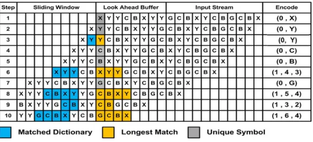
Figure 3.3, the yellow background colored block represents matched symbol in the lookahead buffer, and the blue background colored block represents matched symbol in the respective sliding window. For example, in the initial state, the sliding window is empty, so there is no match with the lookahead buffer. As the encoding process goes, in the sixth row, the result is match starting from the position no.4 with consecutive length 3.

(42)

Figure 3.3 The LZSS encoding algorithm.

In some cases, if only match one symbol is matched, we may not encode it as a matched case if the size of matched codeword symbol is still greater than the unmatched one. In other words, the matched codeword does not have coding gain, which result in expansion of the data. Note that in this example, we assume that the sliding window size is 256, the lookahead buffer size is 5, and the bit width of the symbol is 8. Therefore, if there is only one symbol is matched, encoding the symbol into (1, p, l) will lose bits more than (0, s), as shown in Table 3.2. So we choose to encode the symbol into the unmatched case if the matched length is less than 2. Also, due to there are only 4 natural numbers starting from 2 to 5, we only need two bits to represent the match length.

Similarly, the encoding of numbers from 2 to 9 only requires three bits. That’s why we choose 5, 9 as the LA_BF in this experiment.

(43)

Match length

Compression gain

1 -2 bits

2 7 bits

3 16 bits

4 25 bits

5 34 bits

Table 3.2 The compression gain at certain representation

Figure 3.4 Experiment result demonstrating the LZSS compressibility.

The compression ratio is bounded below by

BF LA b

itwidth codeword b

size data input

a size output dat

CR   * _ , _(3.2)

which means that the main parameters that affect CR is b and LA_BF. Owing to the

(44)

3.2.3 Decompression Process

The decoding process resembles the encoding process much. The decoding process can be divided into three parts: decoding, read-out and shift-in. Received codeword is either matched (1, p, l) or unmatched (0, s). If we get an unmatched codeword, the readout result is simply the symbol in the codeword. If we get a matched codeword, we will go to the sliding window position p specified by the codeword, and get the first l symbols from the position p. After the read-out process, we get the decoded output, and at the same time shift the decoded symbols into the sliding window.

3.2.4 LZSS Algorithm Design Parameters

There are three main design parameters of the LZSS algorithm: the sliding window size SW, the lookahead buffer size LA_BF, and the bit width of the symbol b. The lookahead buffer size LA_BF determines how long a match can be consecutively, also known as the maximum match length. The sliding window is the dictionary memory, which means the past history of sequence of symbols. Thus, if the sliding window is not big enough to recall the past data, we may miss the chance of match, and thus compromises the compression ratio. On the other hand, if there are only few kinds of repeating patterns, we won’t need a long sliding window. The bit width of the symbol

(45)

compression, b equals to the number of scan chains. In test response compaction, b equals to the number of cores. The codeword size changes with LA_BF and SW gradually. The codeword consists of the encoding of the position p and the length l plus 1 flag bit. As LA_BF and SW increases, the codeword increases logarithmically.

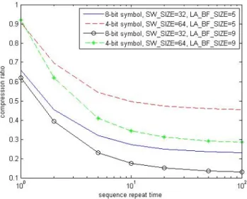
In Figure 3.4, we can see that the compression ratio as the sequence to be compressed repeats more times, the compression ratio becomes better, and gradually reach the compression ratio bound. This also shows that LZSS compression algorithm is better at compressing “symbol patterns” rather than compressing “single symbols”

(like Huffman code or arithmetic code).

(46)

3.3 LZSS-Based Test Stimulus Compression

3.3.1 Don’t-care Bits Filling

After the test patterns are generated using ATPG, there are some don’t-care bits (X’s) in the test patterns. Before the test patterns are applied to the DUT, the don’t-care bits in them should be filled. We can fill the test patterns properly so that the compression ratio can be better. We can use a naïve approach, which fills don’t-care bits according to the neighbor specified bits, which is called adjacency filling to fill the don’t-cares, as shown in Figure 3.6. Because we use a lossless compression algorithm, we can keep the fault coverage while the other approaches might discard unused patterns, which degrades the fault coverage.

Figure 3.5 Proportion of don’t-care bits in 200 test stimulus patterns of the s38417 benchmark circuit

(47)

Figure 3.6 Naïve don’t-care bits assignment using adjacency filling.

3.3.2 Simulation Settings and Results

We use one of the ISCAS’89 benchmark circuits, s38417, as our design under test, and we generate test patterns for it. The ATPG results are shown in Table 3.3, including the number of test patterns and the fault coverage (FC).

In Figure 3.7, the compression ratio becomes better as the proportion of don’t-care bits increases. We can see that when the don’t-care bits proportion reaches 95% or above, the compression ratio falls below 0.5, and the compression is not good when the don’t-care proportion is inadequate.

Also, the compression ratio becomes worse as the lookahead buffer size becomes larger. It’s because increasing the lookahead buffer size not only increases the maximum consecutive matches, but also increases the codeword size. Therefore, the most suitable lookahead buffer size in this case is 5.

(48)

Table 3.3 Simulation setting of test stimulus compression.

Figure 3.7 Experiment of test stimulus compression: fill the test stimulus don’t-care bits using adjacency filling.

(49)

3.4 LZSS-Based Test Response Compaction for Identical Multiple Cores

3.4.1 Validation of Suitability

We assume that the identical multicore system has N cores, where each core having different probabilities of error. The probabilities of error of all cores pi, i=1,…,N, are modeled as i.i.d. exponential random variables with parameter λ, as shown in Figure 3.8. We assume that λ=0.025 as an example in this experiment, and the histogram of probabilities of error is shown in Figure 3.9. In the test response patterns of every core, we use the probability of error to randomly flip the response data at the probability of pi to model the faulty test response, as shown in Figure 3.10.

(50)

Figure 3.9 The histogram of core error probability in this experiment.

Figure 3.10 The formation of an LZSS symbol for test response compaction.

(51)

Figure 3.11 The histogram of compression ratio result of 100 test patterns, each with length of 1024 bits.

Each LZSS symbol is formed by grouping test bits of all the in the respective same scan chain at a time slot, as shown in Figure 3.10. Therefore, each symbol in the LZSS compressor is the same as the number of cores in the system, which is 64 in this experiment. We then feed the test bits into the LZSS encoding algorithm. We randomly generate bits of length 1024, which are the bits of the test response, and flip every bit of each core with the probability of errors as specified above. We repeat the experiment for 100 times. The setting of the LZSS encoding experiment is shown in Table 3.4.

The result of the compression of test patterns is shown in Figure 3.11. We can see

(52)

Table 3.4 The settings of Experiment 1.

Testing configuration

Test pattern length 1024 bits

Number of test patterns 100

Multicore parameters

Number of cores (N) 64

Core error probability parameter (λ) 0.002 LZSS design parameters

Lookahead buffer size 8 symbols Sliding window size 192 symbols

Figure 3.12 The compression ratio versus the error rate parameter λ and core count N.

(53)

There is a subtle relationship between CR and the core error rate parameter λ and core count N, as shown in Figure 3.12. We can see that as the core error parameter decreases from 0.01 to 0.0005, the compression ratio decreases. Also, we can see the general trend that, as the core count N increases from 12 to 64, CR first decreases dramatically, and then rises gradually. This phenomenon arises from the saturation of the redundancy of LZSS symbols. Recall that the core number N maps to the bit width of the symbol in the LZSS compression algorithm. Initially as N is very small (such as 12 in this case), we cannot obtain patterns of similar error cores. As the core number grows, there are more identical symbols, which means identical error outputs. Finally, this effect saturates, and the average codeword size increases as the bit width of the symbol N increases, which degrades CR.

3.4.2 Determination of Design Parameters

We need to determine the design parameters of the LZSS encoding engine to maximize the

compression ratio CR under reasonable hardware constraints. A large sliding window and lookahead

buffer can help match more symbols, and therefore improve CR. But the hardware cost as well as the

(54)

Table 3.5 The settings of experiment 2.

Testing configuration

Test pattern length 1024 bits

Number of test patterns 100

Multicore parameters

Number of cores (N) 16

Core error probability parameter (λ) 0.025 LZSS design parameters

Lookahead buffer size 2,3,5,9,17 symbols Sliding window size 64, 128, 256, 512, 1024 symbols

Figure 3.13 The compression ratio result as LA_BF and SW varies.

(55)

The simulation result of this experiment shows that the compression ratio saturates at the point of (LA_BF, SW) = (5, 1024) in the design space of LZSS, as shown in Figure 3.13. In addition, when we consider the hardware area overhead of the compactor, we know that larger lookahead buffer as well as larger sliding window requires more hardware overhead. Therefore, we choose the point where the CR has diminished return, which is (LA_BF, SW) = (5, 256). Also in Figure 3.13, we can see that, in this specific setting of lookahead buffer size and sliding window size, the compression ratio can be below 0.5 when the core error rate parameter λ is below 0.025.

3.5 Summary

In test stimulus decompression, we can see that the decompressor reaches a compression ratio of about 50% under 95% proportion of don’t-care bits in test patterns.

The test response compactor can achieve compression ratio of less than 0.5 when there are 16 cores with the core error rate parameter λ=0.025. As for design parameters, the lookahead buffer should be long because there might be long consecutive matches.

Increasing LA_BF can improve the compression ratio, at the small cost of codeword

(56)

(57)

Chapter 4 Hardware Architectures for Test Stimulus Decompressors and Test Response Compactors

4.1 Hardware Architecture for Test Stimulus Decompressor

4.1.1 LZSS Decoder Architecture

The LZSS decoder is a simple and direct implementation. The decoding cycle consists of three stages: codeword decomposition, symbols read-out, symbols shift-in.

At the first stage, the translation process, the read-out circuit translates the codeword into match flag, symbol, index and match length. At the remaining stages of the decoder, including the read-out and the shift-in stages, operates on a constant cycle-by-cycle

(58)

Figure 4.1 Hardware architecture for LZSS decoder.

Figure 4.2 The finite state machine (FSM) of the decoder.

Figure 4.3 The timing diagram of LZSS decoder.

(59)

Using the property of continuous output to the scan chains, we design the finite state machine (FSM) of the decoder, as shown in Figure 4.2. The finite-state-machine (FSM) of the decoder contains only three states: initialization, decode and output. The system begins at the initialization state. While there are remaining symbols to be output, the FSM stays in the output state; else, the next state of the FSM goes back to the decoding state, and accept the next codeword. That is to say, there are continuous output cycle feeding into the scan chain. This can comply well with the conventional scan chain architecture, where in each cycle the scan chain feeds in one bit.

Figure 4.4 Symbol combining for shared mux control input.

(60)

4.1.2 Speed Limitations and Optimal Design

The stack of large address decoders (large multiplexers) in the read-out circuit is the main source of the critical path delay. Due to the feedback loop in the critical path, unfolding cannot increase the throughput because the critical path delay also increases as the unfold factor J increases. In other words, the circuit timing is limited to the iteration bound. The only optimization can be done in architectural level is the sharing of selection signals for the decoder mux. As shown in Figure 4.4, for every sliding window position, we fetch the symbol in that position of the sliding window, followed by consecutive LA_BF-1 symbols. This eliminates the hardware (signal wire) for generating LA_BF signals at max.

4.1.3 Implementation Results

We use design compiler to synthesize our decoder with TSMC 0.13μm process.

The synthesis result is shown in Table 4.1. The LZSS-based decoder hardware using this architecture can reach a throughput of 0.278~1.39 GB/s throughput.

(61)

We do the back-end place-and-route of the test stimulus decompressor using SoC Encounter. The decoder hardware after APR is shown in Figure 4.5 and Table 4.2. The die size is about 0.56mm×0.55mm, and can operate at a frequency of 250MHz, and gives a symbol processing rate of 250MB/s.

Table 4.1 Synthesis result of LZSS decoder.

Figure 4.5 The chip layout of LZSS decoder design core.

(62)

Table 4.2The implementation result of LZSS decoder.

(a)

(b)

Figure 4.6 Content addressable memory (CAM): (a) The whole CAM architecture and (b) a cell of the CAM.

(63)

4.2 Review of LZSS Encoder Design

4.2.1 CAM-based LZSS Encoder

Content-addressable memory is a kind of memory with “match” operation. The circuit shown in Figure 4.6(a) is an analog implementation of CAM. The analog CAM cell shown in Figure 4.6(b) is an ordinary SRAM cell plus three transistors dedicated for match operations. The CAM-based LZSS codec in related work [15] utilizes the intrinsic comparison function in the CAM to do fast comparisons. The hardware does parallel comparisons in a single cycle, and therefore have high throughput.

(64)

(a)

(b) (c)

Figure 4.7 Systolic-array-based LZSS encoder: (a) the systolic array architecture; (b) the space-time diagram of (a); (c) the processor element of each circle of (a).

4.2.2 Systolic-array-based LZSS Encoder

The systolic array performs comparison on a cycle-by-cycle basis, which means that the comparison process of one string is distributed into multiple cycles, as shown in Figure 4.7. [18] The systolic array design starts with a pre-map dependence graph (DG). Using proper scheduling vector and projection vector, we can trade-off the area overhead from the latency. Although this architecture has lower hardware cost, it suffers from lower throughput.

(65)

4.2.3 Comparison

The CAM-based design has the merit of high throughput, low latency. However, it suffers from large area overhead due to the highly parallel comparison hardware. The systolic array-based design has lower area overhead compared with the CAM-based design, but the throughput is lower and the latency is higher. Because the we do not want the test compression circuit to degrade the speed of the circuit, the compactor must not become the system bottleneck. Therefore we choose the CAM-based hardware architecture, which has higher throughput and lower latency.

4.3 Encoder Hardware Architecture

4.3.1 Proposed Three-stage CAM-based LZSS Encoder

The proposed CAM-based LZSS consists of three main parts, as shown in Figure 4.8. The first part is the sliding dictionary as well as the parallel generation of the match bits. The second part is the parallel string length counter and the comparator tree. The third part is the generation of the codeword.

(66)

Figure 4.8 Block diagram of LZSS encoder architecture.

In the first part, the sliding dictionary uses the CAM-based design as described in the previous section. It compares each set of the sliding dictionary in parallel. Namely, we compare the string _{_SW_j_,_SW_j_₁_,...,_SW_j__LA_{_}_BF_₁_}with _{_LA₀_,_LA₁_,...,_LA_LA_{_}_BF_₁_}for each j

from 0 to SW1. Next, we generate the match bits for each comparison set j, namely )

(

_bit_j_,_i SW_j _i LA_i

match  _  (4.1)

for j from 0 to SW1 and for i from 0 to LA_BF 1.

In the second part, the string length counter counts the consecutive ‘1’ generated by the previous part, and it is immediately followed by a binary maximum selection tree selecting j corresponding to the maximum match.

(67)

In the third part, the codeword is generated according to whether there is a string match or not. If there is a match, the codeword is encoded in the form of 1, position, length , and is encoded in the form of 0, symbol if there is no match.

The bit width of position p is ⌈log2(SW)⌉, and the bit width of maximum match length l is ⌈log2(LA_BF-1)⌉. The shift operation of the sliding dictionary is also done at the

clock edge of each clock cycles.

The following is a case study as shown in Figure 4.9(a)-(d). Every row here represents a cycle, and every column here represents a sliding window position. First, we do fully parallel symbol match in each row. Second, calculate the length of matched strings in each column. The accumulated match length is shown in red color. Third, select the maximal match length from each row of sliding dictionary, which means to select the best match in every cycle. Fourth, the best match strings can be encoded by the series of maximal counts, as shown in black border.

(68)

(a)

(b)

(69)

(c)

(70)

4.3.1 Unfolded Three-stage CAM-based LZSS Encoder

Figure 4.10 Unfolding as in the previous case study.

Unfolding is a transformation technique that can be applied to a DSP program to create a new program describing more than one iteration of the original program. [3]

Using unfolding means to trade more hardware area for better data processing rate.

Although the design mentioned above has the property of high speed, it still cannot reach the requirement of at-speed testing. The critical path of the above design is estimated to be about 2.5ns, and therefore the clock speed is about 1/2.5ns = 400MHz.

Because we want the encoder to have a 10Gbit/s throughput, which is the transmission speed of the USB 3.1 standard [24], we can do a J-unfold and J is estimated as

(71)

3.125 00

4 / 1.25 rate

clock nominal

throughput

required  

 MHz

s

J GB . (4.2)

However, using unfolding also increases the critical path, so the operation frequency is less than the original. Therefore, we choose J to be 4.

Figure 4.11 Original sliding window of LZSS encoder.

Figure 4.12 Unfolded sliding window of LZSS encoder.

(72)

Figure 4.13 Parallel comparators of Figure 4.11 and Figure 4.12.

Figure 4.12 shows the architecture of the sliding dictionary and the parallel comparators after doing 4-unfolding. Due to the hardware sharing in the sliding window elements, we only need 3 extra registers for the sliding window and 3 extra registers for the input buffer. Figure 4.14 shows the parallel comparator in the first part and the string length counter in the second part. Because there is a feedback loop in the string length counter, we cannot further do pipelining to enhance the speed, and the path is a candidate for the possible critical path.

In the binary comparison tree of the second part, because the path is all feed- forward without feedback loop in this part, we can pipeline the comparator tree to enhance the critical path. However, we do not want the area overhead due to pipeline registers to become too much, and the critical path is bounded by about 4 stages of comparators plus accumulators, we choose 2 comparator stages per pipeline.

(73)

Figure 4.14 The 4-unfolded parallel comparison logic for the sliding window.

(74)

(a)

(b)

Figure 4.15 (a) The pipelined maximum selection tree with two comparator stages in one pipeline stage, and (b) the structure of each node in (a).

(75)

Figure 4.16 The codeword formation example.

In the third part, we encode the symbol into codewords according to whether there is a match or not. As shown in Figure 4.16, the third part may generate 1 to 4 codewords in one cycle. We use the processed max-length and position form the codeword. We need the information from the string length counter in the previous part to do the correct output. The whole architecture of the third part and the single processing element unit in it are shown in Figure 4.17(a)(b), respectively.

Table 4.3 Synthesis result of the 4-unfold LZSS encoder.

(76)

(a)

(b)

Figure 4.17 (a)(b) The processing element and the best-match encoder.

(77)

Figure 4.18 Proportions of the area in the 4-unfolded LZSS encoder architecture.

Figure 4.19 The encoder design is scalable as the core number grows.

4.3.1 Scalability of LZSS Encoder

The LZSS-based test response compactor is a scalable design. The portion of the hardware architecture that grows with the core number N consists of only about 35%,

(78)

(4.3)

As can be seen in Figure 4.19, as the number of cores grows from 8 to 32 cores, the area overhead per core decreases by 63.0%.

4.3.2 Implementation Results

We synthesize the encoder with design compiler under TSMC 0.13μm process.

The synthesis result is shown in Table 4.3. The synthesis result shows that the 4-unfold LZSS encoder architecture can achieve 2 GB/s throughput at the clock rate of 500MHz.

We do the back-end place-and-route of the test response compactor using SoC Encounter. The encoder hardware after APR is shown in Figure 4.20 and Table 4.4. The die size is about 1.24mm×1.24mm, and can operate at a frequency of 100MHz, and gives a symbol processing rate of 400MB/s.

Figure 4.20 The chip layout of LZSS encoder design core.

(79)

Table 4.4 The implementation result of LZSS encoder.

4.4 Summary

The hardware architecture of LZSS decoder is simple, and can reach throughput of 0.278~1.39GB/s with low latency. The LZSS encoder is a four-unfold architecture, and can reach 1.6 GB/s throughput. The 4-unfold LZSS encoder uses three-stage design, and is a scalable as the number of identical cores under test grows. The 4-unfold LZSS encoder reaches throughput of 1.6 GB/s at the clock frequency of 400 MHz.

(80)

Chapter 5 Conclusion and Future Works

5.1 Main Contributions

In conclusion, this thesis proposes an LZSS-based test compression scheme that is both scalable and feasible for diagnosis purpose for identical multicore systems. The algorithm of the LZSS-based test response compactor utilizes the intrinsic property that identical multiple core systems have correlation between cores. As shown in the simulation, the compression ratio reaches about 50% under the core error rate parameter λ=0.025. The decoder is implemented using TSMC .13μm process and can reach the symbol processing rate of 0.278 GB/s at the clock speed of 278 MHz, and the area is 0.55mm × 0.56mm. The LZSS encoder for test response compaction is implemented using TSMC .13μm process and can reach the symbol processing rate of 0.4 GB/s at the clock speed of 100 MHz, and the area is 1.24mm × 1.24mm. The encoder hardware architecture is also a scalable one. When the number of cores grows from 8 to 32 cores, the area overhead per core drops by 63.0%.

(81)

5.2 Future Directions

In the first direction, we can use Huffman code instead of LZSS in test stimulus compression in order to lower on-chip decoding complexity. Although the encoding of Huffman code is more complex than that of LZSS, its decoding is simpler. Using Huffman code as the test stimulus decompressor hardware can reduce the hardware overhead. Also, due to the prefix-code property of the Huffman code, we can easily parse the encoded bitstream into codewords in the decoding process. Therefore, using Huffman coding in test stimulus compression may be better in test stimulus compression

In the second direction, we can do the test-compression-aware ATPG, which means to generate the test stimulus patterns with don’t-care bits that are more compressible using LZSS algorithm. The source of the don’t-care bits comes from the unspecified bits after running ATPG algorithm targeting some specific faults. We can reorder the scan chain bits to aggregate the don’t-care bits together to improve the compressibility.

(82)

References

[1] L.-T. Wang, C.-W. Wu and X. Wen, VLSI Test Principles and Architectures. Elsevier, 2006.

[2] M. L. Bushnell and V. D. Agrawal, Essentials of Electronic Testing for Digital, Memory & Mixed-Signal VLSI Circuits. Kluwer Academic, 2000.

[3] K. K. Parhi, VLSI Digital Signal Processing Systems: Design and Implementation, John Wiley & Sons, 1999.

[4] Test and Test Equipment, in International Technology Roadmap for Semiconductors (ITRS-2011),

https://www.dropbox.com/sh/r51qrus06k6ehrc/AABnW0tCHso_jKTGwLKyXE Jxa/2011Chapters/2011Test.pdf?dl=0

[5] nVidia, http://international.download.nvidia.com/geforce-com/international/pdfs/

GeForce_GTX_980_Whitepaper_FINAL.PDF

[6] T. Han, I. Choi and S. Kang, “Majority-Based Test Access Mechanism for Parallel Testing of Multiple Identical Cores,” IEEE Transactions on Very Large Scale Integration (VLSI) Systems, vol. 23, no.8, Aug. 2015.

(83)

[7] G. Giles, J. Wang, A. Sehgal, K. J. Balakrishnan, and J. Wingfield, “Test Access Mechanism for Multiple Identical Cores,” in IEEE International Test Conference (ITC’08), 2008.

[8] M. Sharma, A. Dutta, W.-T. Cheng, B. Benware and M. Kassab, “A Novel Test Access Mechanism for Failure Diagnosis of Multiple Isolated Identical Cores,” in IEEE Internationl Test Conference (ITC 2011), 2011.

[9] S. Vangal et al., “An 80-Tile 1.28TFLOPS Network-on-Chip in 65nm CMOS,”

IEEE International Solid-State Circuits Conference (ISSCC), 2007.

[10] J. Howard et al., "A 48-core IA-32 message-passing processor with DVFS in 45nm CMOS," IEEE International Solid-State Circuits Conference (ISSCC), 2010.

[11] TILE-Gx 72 Processor, Mellanox, “TILE-Gx Processor Family,”

http://www.mellanox.com/page/products_dyn?product_family=238, Feb. 2013.

[12] B. Jung and W. P. Burleson, “Efficient VLSI for Lempel–Ziv Compression in Wireless Data Communication Networks,” IEEE Transactions on VLSI Systems, vol. 6, pp. 475–483, Sept. 1998.

[13] S. James and S. Thomas, "Data compression via textual substitution," Journal of

(84)

[14] S. Mitra and K. S. Kim, "X-Compact: An Efficient Response Compaction Technique, IEEE Transactions on Computer-Aided Design of Integrated Circuits and Systems, vol. 23, no. 3, Mar. 2004.

[15] Kun-Jin Lin; Cheng-Wen Wu, "A low-power CAM design for LZ data compression," IEEE Transactions on Computers, vol.49, no.10, pp.1139-1145, Oct 2000.

[16] Lee, C.Y.; Yang, R.-Y., "High-throughput Data Compressor Designs Using Content Addressable Memory," IEE Proceedings - Circuits, Devices and Systems, vol.142, no.1, pp. 69-73, Feb 1995.

[17] N. Ranganathan and Selwyn Henriques, “High-Speed VLSI Designs for Lempel- Ziv-Based Data Compression,” IEEE Transactions on Circuits and Systems-II:

Analog and Digital Signal Processing, vol. 40, no. 2, Feb. 1993.

[18] Shih-Arn Hwang; Cheng-Wen Wu, "Unified VLSI systolic array design for LZ data compression," IEEE Transactions on Very Large Scale Integration (VLSI) Systems, vol. 9, no. 4, pp.489-499, Aug. 2001.

[19] S. Jones, “100 Mbit/s Adaptive Data Compressor Design Using Selectively Shiftable Content-Addressable Memory,” IEE Proceedings-G, vol. 139, no. 4, pp.

498-502, Aug. 1992.

(85)

[20] L. Li, K. Chakrabarty and N. A. Touba, “Test Data Compression Using Dictionaries with Selective Entries and Fixed-Length Indices,” ACM Transactions on Design Automation of Electronic Systems, vol. 8, no. 4, pp. 470-490, Oct. 2003.

[21] J. Ziv ,and A. Lempel, "A Universal Algorithm for Sequential Data Compression,"

IEEE Transactions on Information Theory, vol. IT-23, no. 3, May 1977.

[22] R. Kapur, T. W. Williams, and S. Mitra, “Historical Perspective on Scan Compression”, IEEE Design & Test of Computers, vol. 25, issue 2, pp.115-120, Mar.-Apr. 2008.

[23] M. Bellos and D. Nikolos, "Deterministic Test Vector Compression/Decompression Using an Embedded Processor," in Proceedings 5th European Dependable Computing Conference (EDCC-5), pp. 318-331, Budapest,

Hungary, April 2005.

[24] USB 3.1 Specifications, http://www.usb.org/developers/docs/usb_31_052016.zip [25] B. W. Y. Wei, R. Tarver, J.-S. Kim and K. Ng, “A Single Chip Lempel-Ziv Data

Compressor,” in IEEE International Symposium on Circuits and Systems (ISCAS’93), pp. 1953-1955, vol.3, May 1993.

適用於相同多核心系統的測試壓縮及診斷機制之LZSS壓縮演算法及硬體架構設計

National Taiwan University Master Thesis

LZSS Compression Algorithm and Architecture for Test Compression and Diagnosis of Identical Multicore Systems

致謝

摘要

Abstract

Table of Contents

List of Figures

List of Tables

Chapter 1

Introduction

1.1 VLSI Testing and Test Compression

1.1.1 VLSI Testing

1.1.2 Test Flow and Test Compression

1.1.3 Identical Multicore Test Compression System

1.2 Motivation and Goal

1.2.1 Problem Formulation

1.2.2 The Proposed Test Response Compaction Scheme

1.2.3 Thesis Goal

1.3 Thesis Organization

Chapter 2

Review of Test Response Compaction Techniques

2.1 Related Works

2.1.1 Majority-Based Test Access Mechanism for Parallel

Testing of Multiple Identical Cores

2.1.2 A Novel Test Access Mechanism for Failure Diagnosis of

Multiple Isolated Identical Cores

2.2 Problems of Related Works

2.3 Summary

Chapter 3

LZSS-Based Test Compression for Identical Multiple Core Systems

3.1 System Description

3.2 LZSS Compression Algorithms

3.2.1 Introduction to the Algorithm

3.2.2 Compression Process

3.2.3 Decompression Process

3.2.4 LZSS Algorithm Design Parameters

3.3 LZSS-Based Test Stimulus Compression

3.3.1 Don’t-care Bits Filling

3.3.2 Simulation Settings and Results

3.4 LZSS-Based Test Response Compaction for Identical Multiple Cores

3.4.1 Validation of Suitability

3.4.2 Determination of Design Parameters

3.5 Summary

Chapter 4

Hardware Architectures for Test Stimulus Decompressors and Test Response Compactors

4.1 Hardware Architecture for Test Stimulus Decompressor

4.1.1 LZSS Decoder Architecture

4.1.2 Speed Limitations and Optimal Design

4.1.3 Implementation Results

4.2 Review of LZSS Encoder Design

4.2.1 CAM-based LZSS Encoder

4.2.2 Systolic-array-based LZSS Encoder

4.2.3 Comparison

4.3 Encoder Hardware Architecture

4.3.1 Proposed Three-stage CAM-based LZSS Encoder

4.3.1 Unfolded Three-stage CAM-based LZSS Encoder

4.3.1 Scalability of LZSS Encoder

4.3.2 Implementation Results

4.4 Summary

Chapter 5

Conclusion and Future Works

5.1 Main Contributions

5.2 Future Directions

References