Theory and Applications of Dynamical Systems
Song-Sun Lin
Department of Applied Mathematics National Chiao-Tung University
Hsin-Chu, Taiwan
Part I Cellular Neural Network (CNN)
Chapter 1 Introduction Chapter 2 Local patterns
Chapter 3 One-dimensional CNN
Chapter 4 Spatial disorder of inclined output functions
Chapter 5 Bifurcations and chaos in two-cell CNN with periodic inputs
Chapter 1 Introduction
In December 1995, Prof. L. O. Chua visited National Chiao-Tung University to deliver a key-note speech at an international conference on neural networks. He lectured on the theory and applications of CNN and showed us a 10 × 10 cells CNN chips, [12], [13].
The lecture was very interesting and impressive. At the end of his talk, he discussed some interesting open problems for mathematicians.
During the break, Prof. S. N. Chow introduced me to Leon. Shui-Nee was visiting Tsing-Hua University for one year and was an old friend of Leon and me. I told Leon that I was interested in his problems and asked him to explain them to me further. Next morning, he brought a piece of paper with the hotel’s letterhead, descrbing three open prob- lems. He took some time to describe the problems in great detail to ensure that I had fully understood them. I then began my research on the mathematical foundations of CNNs and a long friendship with Leon.
Leon wants to know about the human brain and try to imitate the brain functions to produce very powerful, universal CNN chips for var- ious applications, such as image processing, patterns recognition and others, and especially in areas in which the digital computers are not so effective.
A typical two-dimensional CNN is of the form (1.1) dxi,j
dt = −xi,j + z + X
|k|,|l|≤1
ak,lf (xi+k,j+l) + X
|k|,|l|≤1
bk,lf (ui+k,j+l), (i, j) ∈ Z2, and
(1.2) xi,j(0) = x0i,j.
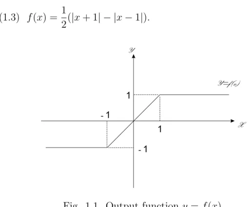
Where the output function f is a piecewise linear function of the form
(1.3) f (x) = 1
2(|x + 1| − |x − 1|).
Fig. 1.1. Output function y = f (x).
A = (akl) is a feedback template, a spatial-invariant template, and B = (bkl) is a controlling template, z is the biased term or threshold.
The quantities xi,j denote the state at cell cij. Figure 1.2 presents the CNN.
Fig. 1.2. CNN
Stationary solutions ¯x = (¯xij) of (1.1) are very important in studying CNNs, their outputs ¯y = (f (¯xij)) are called patterns. Chua and Yang [12] and later Lin and Shih [27] showed that (1.1) behaves like a gradient system when template A is symmetric, meaning that, a−k,−l = ak,l for all |k| and |l| ≤ 1. In this case, every trajectory tends to a stable stationary solution as time passes. For other templates, the trajectories could be periodic, quasi-periodic or chaotic [26], [33].
Among the stationary solutions, the mosaic solutions are stable and are crucial to studying the complexity of (1.1). A mosaic solution ¯x satisfies |¯xi,j| ≥ 1 for all (i, j) ∈ Z2. Its corresponding pattern ¯y = (f (¯xij)) is called a mosaic pattern. In this case, |f (¯xij)| = 1.
Some basic problems in CNN theory can be stated as follows:
(I) Direct problem: Given any P ⊂ P19 = {(z, A, B) : A and B are 3×
3 real matrices and z ∈ R}, determine M(P), the set of all mosaic patterns of (1.1).
(II) Inverse Problem or Learning Problem: Given a set of stationary patterns U, determine a set of parameters P ⊂ P19, such that U = M(P).
(III) Study the complexity of the set of mosaic patterns M(P) for each subset P ⊂ P19.
Given (z, A, B) ∈ P19, the complexity of the set of mosaic pat- terns M(z, A, B) can be studied with reference to spatial entropy. In- deed, on finite lattice Zm×n, the number of mosaic patterns on Zm×n is Γ(m, n; z, A, B). The spatial entropy of M(z, A, B) is defined by
h(M(z, A, B)) = lim
m,n→∞
log Γ(m, n; z, A, B)
mn .
The limit always exists, see [5], [8], [9], [10], [25].
Now, M(z, A, B) exhibits spatial chaos if h(M(z, A, B)) > 0. In this case, Γ(m, n; z, A, B) ∼ ehmn as m, n → ∞. M(z, A, B) describes pattern formation if h(M(z, A, B)) = 0.
The following chapters presents some answers to those problems.
Chapter 2 Local Patterns
This chapter investigates the generation of local patterns for CNN (1.1).
Without a controlling term, the stationary solution to (1.1) satisfies (2.1) −xij + z + X
|k|,|l|≤1
ak,lyi+k,j+l = 0, for (i, j) ∈ Z2.
The methods are illustrated initially by studying one-dimensional CNN with template A = [r, a, s]: equation
(2.2) dxi
dt = −xi+ z + ryi−1+ ayi + syi+1, for i ∈ Z1, and the corresponding stationary equation
(2.3) xi = z + ryi−1+ ayi+ syi+1, for i ∈ Z1.
Firstly, consider the mosaic solution x = (xi) of Eq. (2.3).
If xi ≥ 1, i.e., yi = 1, then
(2.4) (a − 1) + z + ryi−1+ syi+1 ≥ 0.
If xi ≤ −1, i.e., yi = −1, then
(2.5) (a − 1) − z − (ryi−1 + syi+1) ≥ 0.
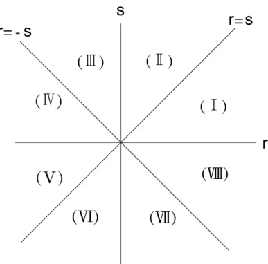
Equation (2.3) has four parameters z, a, r, s. The (r, s)-plane is ini- tially partitioned as follows to solve Eqs. (2.4) and (2.5).
Fig. 2.1. Primary partition of (r, s)-plane.
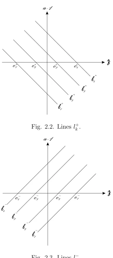
However, in the (a, z)-plane, two sets of four straight-lines are im- portant. The first set is
(2.6) l+k : a − 1 + z + ryl + syr = 0 which is related to (2.4), and the second set is
(2.7) l−k : a − 1 − z − ryl − syr = 0 which is related to (2.5),
here yl and yr ∈ {−1, 1} and 1 ≤ k ≤ 4.
When (r, s) lies in the open regions (I)∼(VIII) the Figs. of (2.6) and (2.7) can be drawn like Figs. 2.2. and 2.3.
Fig. 2.2. Lines lk+.
Fig. 2.3. Lines lk−.
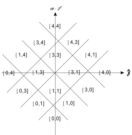
Combining Figs. 2.2 and 2.3, enables the (a, z)-plane to be parti- tioned as in Fig. 2.4.
Fig. 2.4. Partition of (a, z)-plane.
The symbols [m, n] in Fig. 2.4 have the following meanings. Con- sider (r, s) lies in region (I) in Fig. 2.1:
(2.8) r > s > 0.
Denote by
(2.9) C1+ = C4− = −r − s, C2+ = C3− = −r + s,
C3+ = C2− = r − s, C4+ = C1− = r + s
Then, C4+ > C3+ > 0 > C2+ > C1+ are the intersects of li+ and lj− on the z-axis as in Figs. 2.2 and 2.3, respectively.
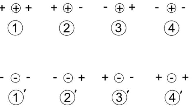
With reference to the local patterns on 3-cells, +1 is represented by the symbol + and -1 is represented by the symbol -.
Under the condition (2.8), the eight local patterns can be listed and ordered as follows.
Fig. 2.5. Ordering of local patterns in region (I).
Now, when (a, z) lies in region [m, n] in Fig. 2.4, the only admissible patterns are exactly, 1° · · · m° and 1°0· · · n°0. For example, when (2.8) holds and (a, z) ∈ [3, 2], then only 1°, 2°, 3°, 1°0 and 2°0 can be pro- duced. This fact is equivalent to the holding of inequalities (2.4) and (2.5) if and only if yi−1, yi, yi+1 are of the form 1°, 2°, 3°, 1°0 and 2°0.
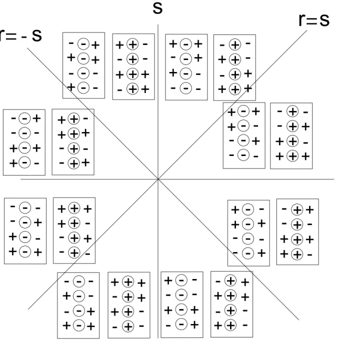
Similarly, in each region from (II) to (VIII), an ordering of eight local patterns on 3-cells can be defined as in Fig. 2.5. Fig. 2.6 presents the complete ordering diagrams. The order are arranged from the first to the fourth as the local patterns run from the bottom to the top. There- fore, for each region from (I) to (VIII), (a, z)-plane can be partitioned into 5 × 5 regions [m, n], as in Fig. 2.4, 0 ≤ m, n ≤ 4.
Fig. 2.6. Orderings of local patterns in (r, s) plane.
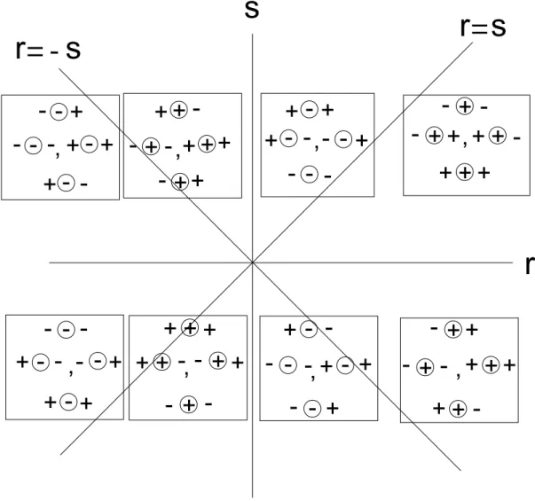
The regions in (a, z)-plane are reduced when (r, z) lies on the bound- aries of open regions in (r, s)-plane. Indeed, when r = s, i.e., A = [r, a, r] is symmetric, then C2+ = C3+ = 0. On the other hand, when s = −r, i.e., A = [r, a, −r] is antisymmetric, then r(+1) + s(+1) = r(−1) + s(−1) = 0, as shown in Fig. 2.7. In these cases, region [m, n]
with m = 2 or n = 2 disappears and then the regions in the (a, z)-plane shrink to 4 × 4 , as shown in Fig. 2.8.
Fig. 2.7. Orderings of local patterns when s = r or s = −r.
Fig. 2.8. Partition of (a, z)-plane when s = r or s = −r.
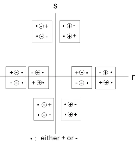
Finally, on the r-axis, where s = 0 and the s-axis, where r = 0. The local patterns are ordered as shown in Fig. 2.9.
Fig. 2.9. Ordering of local patterns on r and s-axis.
The regions [m, n] in which m or n equals 1 or 3 disappear and the number of regions in the (a, z)-plane decreases further to 3×3, as shown in Fig. 2.10.
Fig. 2.10. Partition of (a, z)-plane when s = 0 or r = 0.
Combining the partitions of the (r, s)-plane and the (a, z)-plane, yields the following result for the Direct Problem.
Theorem 2.1 For one-dimensional CNN of Eq.(2.3). There are 200 open subregions Pk, 1 ≤ k ≤ 200, of P4 ≡ {(A, z) : z ∈ R1 and A = [r, a, s] is a 1 × 3 real matrix} such that
(i) P4 =
200[
k=1
Pk, (ii) PkT
Pl = ∅ if k 6= l,
(iii) (A, z) and ( ˜A, ˜z) in Pk for some k if and only if they generate the same local patterns.
The method can be applied to Eq.(2.1), for the two-dimensional problem [18]. In this case, the parameters are z and A which is a 3 × 3 real matrix. The Direct Problem can be solved as follows.
Theorem 2.2. There is a positive integer K and unique set of open subregions {Pk}Kk=1 of P10 = {(z, A) : z ∈ R1 and A is a 3 × 3 real matrix.} satisfying
(i) P10 = [K k=1
Pk , (ii) PkT
Pl = ∅ if k 6= l,
(iii) (A, z) and ( eA, ez) ∈ Pk for some k if and only if they generate the same local patterns.
The result can also be generated for a larger template (2d + 1) × (2d + 1) matrix A, d ≥ 1. For the details see [18].
Chapter 3 One-dimensional CNN
The previous chapter described the generation of local patterns.
This chapter discusses the extension of local patterns to the whole Z1. The two-dimensional case will be discussed in Part II ”Pattern generation problems“ below.
The method for extending to global patterns involves determining the related transition matrix for a given set of local patterns.
For simplicity, only A = [r, a, s] is considered. The set P
3×1 of all local patterns defined on 3-cell can be arranged into the following or- dering matrix X3×1 = [pij]4×4.
Fig. 3.1. Ordering matrix X3×1.
Notably, the symbols - and + are ordered by ¯ < ¢ and then lexicographically for patterns on Zn×1, for n ≥ 2.
Given a subset B ⊂ P
3×1, which is called a basic set, a transition matrix T = T (B) can be introduced as follows, and T = (tij)4×4 is
defined as
(3.1) tij =
½ 1 if pij ∈ B, 0 if pij ∈/ B.
Example 3.1. On [3, 2] of (I), the basic set
B = {− − −, − − +, + + +, + + −, − + +}.
Hence
T =
1 1 0 0 0 0 0 1 0 0 0 0 0 0 1 1
Note that
(3.2) Γn+2 ≡ |Tn| = the sum of all entries in Tn,
and is the number of all admissible pattern on Zn+2, n ≥ 1, which can be generated from T (or B). The spatial entropy is defined as
(3.3) h(T ) = lim
n→∞
log Γn n .
The limit exists and equals log ρ(T ), where ρ(T ) is the maximum eigen- value of T according to the Perron-Frobenius Theorem. When h(T ) >
0, the spatial chaos occurs. When h(T ) = 0, the pattern formation arises. The following theorem indicates which regions in P4 have posi- tive entropy.
Theorem 3.2. The open regions with positive entropy in (a, z) -planes for (r, s) in (I)∼(VIII) are displayed in Fig.3.2, where λi, 0 ≤ i ≤ 4, is the largest root of the polynomial defined by
Q0(λ) = λ − 2, λ0 = 2,
Q1(λ) = λ3 − λ2 − λ − 1, λ1 = 1.839286,. Q2(λ) = λ3 − 2λ2 + λ − 1, λ2 = 1.754877,. Q3(λ) = λ2 − λ − 1, λ3 = g = 1.61803,. Q4(λ) = λ3 − λ − 1, λ4 = 1.324717 .. The entropy in the region is log λi.
Fig. 3.2.
Remark 3.3. The results of Theorem 3.2 can be generalized to any template A = [r1, r2, . . . , rk, a, s1, s2, . . . , sk], k ≥ 1.
Remark 3.4. Given a basic set B ⊂ P
3×1, the exact number ΓB,n of patterns with various boundary conditions-Dirichlet, Neumann and periodic on Zn×1 can be computed, [7].
Chapter 4 Spatial disorder of inclined output function
In the previous chapter, the output function f (x) is flat in the range
|x| > 1. This chapter considers the output function f (x) which is non- flat in the range |x| > 1. It produces some interesting new phenomena including spatial entropy [1], [2], [3], [4], [17].
The general three-piecewise linear output function is defined by
(4.1) f (x) =
mx + k − m if x ≥ 1,
kx if − 1 ≤ x ≤ 1,
lx − k + l if x ≤ −1 where, k > 0 and l, m ≥ 0. Moreover, when k = 1,
(4.2) fl,m(x) =
mx + 1 − m if x ≥ 1,
x if − 1 ≤ x ≤ 1,
lx − 1 + l if x ≤ −1
Furthermore, when k = 1 and l = m, fl,m is symmetric with respect to the origin and is denoted by
(4.3) fm(x) =
mx + 1 − m if x ≥ 1,
x if − 1 ≤ x ≤ 1,
mx − 1 + m if x ≤ −1
fm is studied first. Consider A = [r, a, s] and z = 0 in the stationary equation (2.3):
(4.4) xi = ryi−1 + ayi + syi+1,
for i ∈ Z1. When m > 0, the inverse function gm of fm exists and is given by
(4.5) gm(v) =
1
mv − m1 + 1 if v ≥ 1,
v if − 1 ≤ v ≤ 1,
m1v − 1 + m1 if v ≤ −1
Using the inverse function gm, Eq. (4.4) can be rewritten as (4.6) gm(vi) = rvi−1 + avi + svi+1.
If r = 0 and s 6= 0, then (4.7) vi+1 = 1
s(gm(vi) − avi)
Therefore, Eq. (4.7) describes trajectories of a one-dimensional it- eration map Fm defined by
(4.8) Fm(v) = 1
s(gm(v) − av).
However, if r 6= 0 and s 6= 0, let (4.9) ui+1 = vi,
then (4.6) can be rewritten as (4.10) vi+1 = 1
s(gm(vi) − avi− rui).
Therefore, (4.9) and (4.10) are trajectories of two-dimensional iter- ation map
(4.11) Fm(u, v) = (v, 1
s(gm(v) − av − ru)).
This chapter focuses on the complexity of the one-dimensional map
Fm in (4.8). For two-dimensional map (4.11), when m is positive and sufficiently small, the Smale horseshoe appears, see [17]. For these maps, each bounded trajectory will corresponds to the outputs of bounded stationary solutions. Furthermore, if the maps are chaotic, then the stationary solutions of Eq. (4.4) are spatially disordered. How- ever, only stable stationary solutions of to (4.4) should be considered.
Therefore, the set of all stable bounded orbits Sm of Fm must be con- sidered. If the entropy of Sm is positive, then the stable stationary solutions to Eq. (4.4) represent spatial disorder, or spatial chaos.
The stability considered herein is linear stability. The following def- initions are applied.
Definition 4.1. Let ¯x = (¯xi)i=∞i=−∞ be a stationary solutions to Eq.
(4.4). Then ¯x is called a non-transitional stationary solution if |¯xi| 6= 1 for all i. The linearized operator of these ¯x is defined by
(4.12) (L(¯x)ξ)i = −ξi+ afm0 (¯xi)ξi + sfm0 (¯xi+1)ξi+1
for ξ = (ξi)i=∞i=−∞ ∈ l2. ¯x is called stable if all real parts of the eigenval- ues of L are negative with eigenvector in l2 and unstable otherwise.
Notably, since fm is not differentiable in transition state xi = 1, only non-transitional stationary solutions are considered.
We firstly state the following stability result; for the proof see [19].
Lemma 4.2. Assume a > 1, r = 0 and s > 0 and m > 0. Let
¯
x = (¯xi)i=∞i=−∞ be a non-transitional stationary solution to Eq. (4.4).
Then
(i) if there exists i ∈ Z1 such that |¯xi| < 1, then ¯x is unstable.
(ii) if m(a + s) < 1 and |¯xi| > 1 for all i ∈ Z1, then ¯x is stable.
The stability requires only part of the graph of u = Fm(v) which lie
in {(v, u) : |v| > 1 and |u| > 1} is relevant.
Thus, the map Fm is considered is a gap map associated with the solid part of the graph in Fig. 4.1.
Fig. 4.1. Gap map Fm.
The main result for Eq.(4.4) with an inclined output function can be stated as follow.
Theorem 4.3. Suppose z = 0, r = 0 and s > 0, and a > s+1. Denote (4.13) m∞ = m∞(a, s) = a − s − 1
a(a − 1) + s(a − 2), (4.14) m2 = m2(a, s) = a − s − 1
a(a − 1) + s(a − 1),
and h(m) is the spatial entropy of Fm. Then there exists a strictly decreasing sequence {mp}∞p=2 with
p→∞lim mp = m∞
such that
(i) m ∈ [0, m∞), h(m) = log 2,
(ii) m ∈ [mp, mp−1), h(m) = log λp, where λp is the largest root of
(4.15) λ2p−2− ( Xp−2
i=0
λi)2 = 0.
Moreover, λp is strictly increasing in p with λ3 = g < λp < 2 for p ≥ 4,
(iii) if m2 ≤ m < 1
a + s, then h(m) = 0.
The entropy function h(m) is a step function of m of the form shown in Fig. 4.2. The result of Theorem 4.3 show that the entropy h(m) is a devil-staircase like function and is decreasing in m.
Fig. 4.2. Entropy function h(m).
Proof of Theorem 4.3.
Denote the fixed points of Fm by A, O and D with O = (0, 0),
A = (A1, A2) = ( 1 − m
1 − m(a + s), 1 − m 1 − m(a + s)), D = (D1, D2) = ( m − 1
1 − m(a + s), m − 1
1 − m(a + s)) = −A, and B = (1, Fm(1)) and C = (−1, Fm(−1)),
i.e.,
B = (B1, B2) = (1,1
s(1 − a)), C = (C1, C2) = (−1,1
s(a − 1)).
The theorem is proven by verifying that mp satisfies (4.16) Fmp−1p (a − 1) = 1,
and Fmp(v) has 2p periodic cycle {Fmi p(c)}2p−1i=0 , for p ≥ 2.
For simplicity, the proof for p = 2 and p = 3 are sketched, for p ≥ 4, see [19].
When p = 2, then m2 is given by
(4.17) a − 2
a(a − 1),
and R+1(m2) = a − 1. Then, there is 4-periodic cycle staring from C following by R+, B, L− and back to C, see Fig. 4.3. The four stable subintervals Ij, 1 ≤ j ≤ 4, have the following covering relation
I1 → I2, I4 → I3, I2 → I3, and
I3 → I2.
The transition matrix M(2) of the stable subintervals is given by
(4.18) M(2) =
0 1 0 0 0 0 1 0 0 1 0 0 0 0 1 0
.
Hence, the entropy h(m2) = 0.
u=T(v) u=v
A
v u
B C
D
1 -1 O
R+
R- L+
L-
I1
I I 2
I4 3
Fig. 4.3. Graph Fm2(v) and its stable subintervals.
For p = 3, the graph and Fm3(v) and its subintervals are given in Fig. 4.4. The covering relation for 2p stable subintervals are given by
(4.19)
I1 → I2 → · · · → Ip−1 → Ip,
I2p → I2p−1 → · · · → Ip+2 → Ip+1, Ip → Ik f or k = p + 1 to 2p − 1, Ip+1 → Ik f or k = 2 to p.
In particular, for p = 3
I1 → I2 → I3, I6 → I5 → I4, I3 → I4∪ I5, and
I4 → I2 ∪ I3. Therefore, the transition matrix is
(4.20) M (3) =
0 1 0 0 0 0 0 0 1 0 0 0 0 0 0 1 1 0 0 1 1 0 0 0 0 0 0 1 0 0 0 0 0 0 1 0
6×6
.
The entropy h(m3) = log λ3, λ3 satisfies λ4 − (λ + 1)2 = 0, as in (4.15).
u=T(v) u=v
A
v u
B C
1 -1 O
R+
R- L+
L-
I1
I I3 2
I4
D
I6I5
Fig. 4.4. Graph Fm3(v) and its stable subintervals.
Remark 4.4.
(i) When the biased term z 6= 0, the Fm is no longer symmetric with respect to the origin. However, results like those from Theorem 4.3 were obtained in [2].
(ii) When the output function is asymmetric, i.e., fl,m with l 6= m.
The situation is much more complicated. For z = 0, the entropy function h(l, m) has already been studied in [1]. Now, the devil- staircase-like behavior is exhibited in both l and m directions.
Chapter 5 Bifurcations and chaos in two-cell CNN with periodic inputs
This chapter studies the bifurcation and temporal chaos in two-cell CNN with periodic inputs.
Consider the following two-cell CNN with input:
(5.1)
½ x˙1 = −x1 + ay1 + sy2 + bu(t),
˙
x2 = −x2 + ry1 + ay2,
where the feedback template A = [r, a, s] satisfies (5.2) a > 1, a − 1 < r and a − 1 < −s.
It is easy to verify that condition (5.2) implies that there exists a limit cycle Λ0(A) to (5.1) when b = 0.
The input function (or forcing function) is (5.3) u(t) = sin 2π
T t
with period T > 0 and amplitude b > 0.
The main theme in studying (5.1) is to find out appropriate inputs such that complicated attractors appear. Indeed, Zou and Nossek [33]
discovered a ladyshoe type chaotic attractor when (5.4) A = [1.2, 2, −1.2], T = 4 and b ∼= 4.08.
In this chapter, we recover their results and study more general situation.
The programs for studying bifurcation and chaos are as follow.
(I) Take b = 0 and study how the sustained limit cycles Λ0(A) vary with the template A = [r, a, s]. The existence and uniqueness of
limit cycles will be studied.
(II) Fix template A = [r, a, s], find possible range of input periods T such that (5.1) exhibit chaotic behavior for suitable b > 0. In particular, try to find the relation between T and T0(A) such that (5.1) have complex trajectories for some b > 0.
(III) Fix A and T obtained in (I) and (II), try to identify critical num- bers of b, say, b∗0 < b∗1 < . . . < b∗k, which represent various types of trajectories of (5.1) and may cause distinct bifurcations when b∗j is crossing.
In section 5.1, the existence and uniqueness problem of periodic cycle to Eq. (5.1) when b = 0 is considered. In section 5.2, the bifurcations precede chaos is discussed. The FFT is used to study periodic and quasi-periodic attractors. In section 5.3, the temporal chaos is investi- gated. The effects of input period T can be studied by examining the asymptotic limit cycle Λ∞(T, A) with period T . Then, the study focus on (i) effect of the input amplitude, (ii) effect of the input period and (iii) effect of the varying templates.
§ 5.1. Limit cycles
This section discusses the existence and uniqueness of limit cycle to Eq. (5.1) when b = 0. Since the nonlinear output function f is piecewise linear, the phase-plane R2 can be divided into nine regions which are the mosaic (saturated) region Mj, the transitional (partial saturated) region Tj, and the interior (not saturated) region I, j = 1, 2, 3, 4, as in Fig. 5.1.
Fig. 5.1.
It is easy to see that periodic orbit does not lie entirely in the inte- rior region I. Therefore, periodic orbits have to intersect the exterior region E, here
(5.5) E = R2 − I = [4 k=1
Tk ∪ Mk.
A periodic orbit Λ is called an exterior (periodic) cycle if Λ ⊆ E, oth- erwise Λ is called a non-exterior cycle, i.e., ΛT
I 6= ∅.
We firstly present the following result.
Theorem 5.1. Assume (5.2) and b = 0, then (i) limit cycles exist,
(ii) no more than two limit cycles are present in the exterior region E, and
(iii) if 1 < a ≤ 2, then at most one exterior limit cycle exists.
The multiplicity of exterior limit cycle can be stated as follows.
Theorem 5.2. Assume (5.2) and b = 0, define function (5.6) R(r, a, s) = δ{(−δ + s
aξ)(η − ξκq) + (η − γδη
aξ )(δ − γχq) +(−rs
a2 + rδ
aξ)(η − ξκq)(δ − γχq)}, where
(5.7)
ξ = r − a + 1, η = r + a − 1, γ = 1 − s − a, δ = a − s − a, q = 1
a − 1, κ = ξ
η and χ = r δ. Then,
(i) there is a unique exterior limit cycle if R > 0, and (ii) there is no exterior limit cycle if R < 0.
When A is antisymmetric, i.e., −s = r, R(r, a, s) can be reduced to (5.8) R(r, a) = (a(a − 1) + r2 − r) − κq(a(a − 1) + r2 + r).
Proof of Theorem 5.1.
(i) Under the assumptions (5.2), the origin O = (0, 0) can be easily verified to be the only steady state of (5.1), moreover, O is an unstable spiral. Indeed, the associated eigenvalues at O are given by
λ± = a − 1 ± i√
−rs.
By Poincar´e-Bendixson Theorem, a limit cycle exists. Apart from the origins, all trajectories will tend to one of the limit cycles as t → ∞.
Fig. 5.2. A typical orbit of (5.1) with initial condition (α, −1), and 1 ≤ α ≤ a − s.
(ii) Periodic solutions as in Thiran [32] are constructed to show that no more than two periodic orbits exist in exterior region E.
Now starting at the point (α, −1) at t = 0, where 1 ≤ α ≤ a − s, the trajectory Γα in T1 is followed; it intersects x2 = 1 at the point (α1, 1) on t = t1, 1 < α1 , enters M1; then intersects x1 = 1 at
(1, β2) on t = t2, enters T2; then intersects x1 = −1 at the point (−1, β3) on t = t3, and finally enters M2 and intersects x2 = 1 at the point (α4, 1) on t = t4, i.e.,
(5.9)
( x1(0), x2(0)) = ( α, −1), (x1(t1), x2(t1)) = ( α1, 1), (x1(t2), x2(t2)) = ( 1, β2), (x1(t3), x2(t3)) = (−1, β3), (x1(t4), x2(t4)) = ( α4, 1),
see Fig. 5.2. Since b = 0, (5.1) is an autonomous equation. The periodic orbit cannot intersect itself. Therefore, by (i), Γα is a periodic (closed) orbit if and only if
(5.10) α4 = −α.
α1, β2, β3, α4 and t1, t2, t3, t4 must be computed in terms of α. The following expressions can be straight-forwardly obtained. The de- tails are omitted here. It is easy to verify
(5.11) α1 = a + s(1−r)a + (α − a + s(r+1)a )(ηξ)q, (5.12) β2 = a + r − α ηγ
1−a−s,
(5.13) β3 = a − r(s+1)a + (β2 − a − r(1−s)a )(γδ)q, (5.14) α4 = β δξ
3+r−a + s − a.
α4 is written as a function of α to show that (5.10) has at most two solutions for α ∈ [1, a − s]. Indeed, in the following, ki, i = 1, · · · , 17, are constants that depend on a, r, s, but are independent
of α,
α1 = k1α + k2 , β2 = k4
k1α + k3 + k5 , β3 = k6β2 + k7 , α4 = k9
β3 + k8 + k10 , and
(5.15) α4 = k9α + k13
k11α + k12 + k14.
Substituting (5.15) into (5.10) yields, a quadratic equation for α, i.e.,
k15α2 + k16α + k17 = 0.
Therefore, (5.10) has at most two solutions in [1, a − s].
(iii) Note that
(5.16) ∂
∂x1(−x1 + ay1 + sy2) + ∂
∂x2(−x2 + ry1 + ay2)
=
½ a − 2 if (x1, x2) ∈ Ti ,
−2 if (x1, x2) ∈ Mi ,
1 ≤ i ≤ 4. The sign is nonpositive if a ≤ 2. The Dulac criteria rule out the second closed orbit in E. The proof is complete. ¥ To prove Theorem 5.2, it sufficies to prove following theorem.
Theorem 5.3. Assume (5.2) and b = 0. Let ξ, η, γ, δ and q be
given by (5.7).
(i) There is a periodic cycle in the exterior region E if the following conditions are satisfied.
(E1) a − 1 + s(1 − r)
a + (1 − a + s(r + 1) a )(ξ
η)q ≥ 0 ,
(E2) a − 1 − r(1 + s)
a + (1 − a − r(1 − s) a )(γ
δ)q ≥ 0 .
In particular, if A is antisymmetric, i.e., −s = r, (E1) and (E2) is equivalent to
(E) a(a − 1) + r(r − 1) − [a(a − 1) + r(r + 1)](ξ
η)q ≥ 0.
(ii) There is no periodic orbit in the exterior region E if one of the following conditions holds.
(N1) a − 1 + s(1 − r) a + sξ
a (ξ
η)q < 0 , or
(N2) a − 1 − r(1 + s)
a − rγ a (γ
δ)q < 0 .
In that case, all periodic cycles are necessary intersect the interior region I.
Proof.
The existence results are first proved.
It is easy to verify that if Λ is an exterior periodic cycle then ΛT
{(x1, −1)|x1 ∈ [1, a − s]} 6= ∅.
From (5.7) and (E1),
α1(α) ≥ 1 for all α ∈ [1, a − s] .
Similarly, from (5.13) and (N1),
β3(β2) ≥ 1 for all β2 ∈ [1, a + r] .
Therefore, x1(α, 1) maps [1, a−s] into [−a+s, −1]. It implies −x1(α, 1) maps [1, a − s] into itself and then has a fixed point in [1, a − s]. Hence, (5.10) has at least one solution in [1, a − s]. This proves that exterior periodic cycle exists.
Clearly, (E1) and (E2) is equivalent to (E) when s = −r.
Finally, from (5.12) and (N1),
α1(α) < 1 for all α ∈ [1, a − s] , and from (5.13) and (N1),
β3(β2) < 1 forall β2 ∈ [1, a + r] .
Hence, there is no exterior periodic cycle exists. The proof is complete.
¥
Notably, (N1) and (N2) can be replaced by stronger conditions that can be verified easily as follows.
0 < a − 1 < r < 1 and − s ≥ a(a − 1) 1 − r , and
0 < a − 1 < −s < 1 and r ≥ a(a − 1) 1 + s .
§ 5.2. Bifurcation Precede chaos
Intuitively, when the amplitude b of input bu(t) is small, period T is different from the period T0 of sustained limit cycle, then the (5.1) may have complicated trajectory like quasi-periodic but not chaotic.
Therefore, in the section, the impact of an input bu(t) on its period T and amplitude b are studied for the bifurcation phenomena before chaos occurs.
Consider (5.1) with initial conditions (5.17) x1(0) = ξ1 and x2(0) = ξ2. The solution of (5.1) and (5.17) is denoted by
(x1(t, ξ1, ξ2), x2(t, ξ1, ξ2)),
where xi(t, ξ1, ξ2) ≡ xi(t, ξ1, ξ2; b, T, A), i = 1 and 2.
The ω-limit set of (5.1) is denoted by
(ω(ξ1, ξ2; b, T, A)),
and the nonwandering set of (5.1) is denoted by
(5.18) Ω(b, T, A) = ∪ω(ξ1, ξ2; b, T, A), (ξ1, ξ2) ∈ R2.
Since the input is T -periodic, for a fixed parameter A, T and b, a two-dimensional Poincar´e map of (5.1) can be defined as
(5.19) F (ξ1, ξ2) = (x1(T, ξ1, ξ2), x2(T, ξ1, ξ2)).
Now, the study of the bifurcations problem of (5.1) is equivalent to the study of how Ω(b, T, A) changes when b, T and A vary.
In general, it is hard to identify Ω(b, T, A) and to know how it changes. Therefore, we concerned mainly with how ”typical“ trajec- tories vary with b, T, A. In our problem, a typical trajectory Γb ≡ Γ(b, T, A) and ω-limit set ωb = ω(b, T, A) are chosen of (5.1) with the initial condition at the origin O = (0, 0). The ω-limit set of Poincar´e map is denoted by ˆω(b, T, A).
To show Ω(b, T, A) is a chaotic attractor, the following conditions must be proven to hold
(i) Γ(b, T, A) have a positive Lyapunov exponent, (ii) ˆω(b, T, A) is fractal,
(iii) FFT (Fast Fourier Transform) of Γ(b, T, A) have a broad-band.
We first use FFT to study (5.1). Let Λ0 be the sustained limit cycle for b = 0 and is obtained from Theorem 5.1. Apply FFT to the x1- component of Γb, i.e., x1(t, 0, 0), t > 0. Pick up the first N frequencies of these data, i.e., let {akeiωkt}Nk=1 satisfy
(5.20) |a1| ≥ |a2| ≥ . . . ≥ |aN| ≥ |aω|
for other frequency ω, where ak = ak(b) and ωk = ωk(b). Denote (5.21) τk(b) = 2π
ωk(b),
the period of the kth mode. For simplicity, denote (5.22) Tb = τ1(b),
which corresponds to the largest amplitude except for T -mode.
Let aT = aT(b, T, A) be the amplitude of the period T mode. The ratio
(5.23) A(b) ≡ |aT(b)|
|a1(b)|
represents the relative strength of the T -mode with respect to the Tb- mode as b varies. Equation (5.1) is called Tb dominant if A(b) ¿ 1, the Tb and T modes are comparable if A(b) ' 1 but T is dominant if A(b) À 1.
It is not difficult to verify
(5.24) lim
b→0+Tb = T0. The normalized curves (5.25) Rk(b) = τk(b)
Tb
of τk(b), 1 ≤ k ≤ N, are very useful for finding periodic orbits. To be more specific, in the ZN-(Zou-Nossek) case, Rk(b) with 1 ≤ k ≤ 20 and b ∈ [0, 4] are as in Fig. 5.3.
0 0.5 1 1.5 2 2.5 3 3.5 4 0
0.1 0.2 0.3 0.4 0.5 0.6 0.7 0.8 0.9 1
t
4a a
b
4p
Fig.5.3. FFT of the largest 20 modes for the ZN-case : A = [1.2, 2, −1.2] and T = 4.
(1) The amplitude of the T = 4 mode (represented by a red thick line in Fig. 5.3) grows steadily as b increases in (0, 3.826). It is comparable to Tb when b is close to 4, near the onset of chaos.
(2) Curve number 2° decreases and curve number 3° increases and merges into Tb/2 and giving rise to 4T periodic cycles. The 4T cy- cle will survive for quite a large range of parameters in (0.43, 0.66).
Curves merging is very common and induces a period cycle.
(3) The Tb/3 mode maintains the largest parameters in (0, 3.826) and
gives rise to a 3T periodic cycle in (1.2, 3.826).
(4) The dotted regions and window regions (stepped regions) inter- weave with each other. Stepped regions represent periodic cycles and dotted regions represent quasi-periodic orbits.
In the ZN-case, when b ≥ 3.826, the strength of the T -mode is comparable with or larger than the strength of the Tb-mode. In the following, a heuristic argument is used to derive relations among for b, T and T0 when Tb and T are comparable.
Let
(5.26) γ(t) = Λ00(t + t0),
Λ0(t) be the limit cycle of (5.1) with b = 0. The first equation of (5.1) is modelled as
(5.27) dx
dt = γ(t) + bu(t).
Now, γ(t) is a periodic function with period T0 and u(t) is a period function with period T . The two time scales of the functions γ and u can be normalized to a single time scale τ ∈ [0, 1] by setting t = T0τ for γ and t = T τ for u. Hence,
(5.28) x(t) = x(0) + T0Γ(τ ) + bT U(τ ) , τ ∈ [0, 1] , where
Γ(τ ) =
Z T0τ
0
γ(s)ds and U(τ ) = Z T τ
0
u(s)ds
are normalized periodic functions with period one. From (5.28), x(t) can very maximally if T0 and bT have the same order of magnitudes and an appropriate time shift t0 occurs in (5.28). Therefore, for a fixed
template A = [r, p, s], let T0 = T0(A) be the period of the sustained limit cycle Λ0(A) (without input), define
(5.29) b∗(T ) = c0T0(A)
T ,
where c0 ∼ 1 is a constant that depends on A and T .
From our experiences, for a given A and T , c0 = 1 in (5.29) is a good guess for the position at which to start the search for interesting ranges of b. c0(A, T ) may decrease as T increases. In the ZN-case and many other templates, (5.29) worked very well. See Fig. 5.4.
−6 −4 −2 0 2 4 6
−6
−4
−2 0 2 4 6
x1 x2
x cp
cm o
−6 −4 −2 0 2 4 6
−6
−4
−2 0 2 4 6
x1 x2
x cp
cm
(a) b∗1 = 3.98 (b) b∗2 = 4.284
−6 −4 −2 0 2 4 6
−6
−4
−2 0 2 4 6
x1 x2
x cp
cm
−6 −4 −2 0 2 4 6
−6
−4
−2 0 2 4 6
x1 x2
x cp
cm
(c) b∗3 = 4.365 (d) b∗2 = 4.2697 Fig. 5.4. Critical trajectories of b∗1, b∗2, b∗3 and b∗, when
A = [1.2, 2, −1.2] and T = 4.
Let b∗0 > 0 such that
(5.30) |a1(b, T, A)| > |aT(b, T, A)|
hold in (0, b∗0), b∗0 can be assumed to be the least upper bound of ˜b such that (5.30) holds in (0, ˜b).
When a periodic window appears on the open interval B ⊂ (0, b∗0) ,
the curve Rk(b) will be a horizontal lines, or approximately one, on B.
Furthermore, on B
(5.31) Tb = mnT
for some positive integers m and n and (m, n) = 1, i.e., m and n are relative prime. Therefore,
(5.32) Bm,n = {b ∈ (0, b∗0)|Tb = mnT } is defined. Denote by
(5.33) [T0/T ] = m∗ ,
where [x] is the largest integer which is equal to or smaller than x.
The solutions of (5.1) can be written explicitly on each of the nine regions Mj, Tj and I. Therefore, the exact solutions of periodic or- bits in Bm,n can be rigorously checked using a computer provided n is not too large. The periodic cycles in Bm,n are of period mT and cir- cle around the origin O n-times (n-copies). This explanation partially prove of the following results.
Conjecture 5.4. Assume (5.30) holds.
Then
(i) Bm∗,1 6= ∅, i.e., a stable m∗T periodic cycle of (5.1)exists.
(ii) If (5.1) has another stable limit cycle with m∗T period in Bm∗,n∗ ⊂ (0, b∗0) and m∗/n∗ < m∗, then ∪m∗/n∗≤m/n≤m∗Bm,n is open and dense in (ˆb1, ˆb2), where ˆb1 = inf Bm∗,1 and ˆb2 = sup Bm∗,n∗, i.e., Tb as a function of b is a devil’s staircase in b. See Fig. 5.5.
0 0.5 1 1.5 11
12 13 14 15 16 17 18
x
0 0.5 1 1.5 2 2.5
13.5 14 14.5 15 15.5 16 16.5 17 17.5
x
(a) T = 4 (b) T = 2
Figure 5.5. Devil’s staircase like period function Tb, A = [1.2, 2, −1.2], (a) T = 4 and (b) T = 2.
−6 −4 −2 0 2 4 6
−6
−4
−2 0 2 4 6
x1 x2
x
−6 −4 −2 0 2 4 6
−6
−4
−2 0 2 4 6
x1 x2
x
(a) b = 0.5, Tb = 4T (b) b = 0.78, Tb = 154 T
−6 −4 −2 0 2 4 6
−6
−4
−2 0 2 4 6
x1 x2
x
−6 −4 −2 0 2 4 6
−6
−4
−2 0 2 4 6
x1 x2
x
(c) b = 0.9, Tb = 113 T (d) b = 1, Tb = 72T
−6 −4 −2 0 2 4 6
−6
−4
−2 0 2 4 6
x1 x2
x
−6 −4 −2 0 2 4 6
−6
−4
−2 0 2 4 6
x1 x2
x
(e) b = 1.1, Tb = 103 T (f) b = 1.2, Tb = 3T Fig. 5.6. Some typical orbits in Bm,n prior to chaotic regions,
A = [1.2, 2, −1.2] and T = 4.
−4 −3 −2 −1 0 1 2 3 4
−4
−3
−2
−1 0 1 2 3 4
x
−4 −3 −2 −1 0 1 2 3 4
−4
−3
−2
−1 0 1 2 3 4
x
(a) b = 0.37 (b) b = 0.37
−4 −3 −2 −1 0 1 2 3 4
−4
−3
−2
−1 0 1 2 3 4
x
−4 −3 −2 −1 0 1 2 3 4
−4
−3
−2
−1 0 1 2 3 4
x
(c) b = 1.14 (d) b = 1.14
Figure 5.7. Some typical quasi-periodic orbit (a) and (c) and their ω-limit set ˆω of the Poincar´e map (b) and (d),
A = [1.2, 2, −1.2] and T = 4.
§ 5.3. Chaos
This section discusses the chaotic phenomena that occurs when the strength of Γb and input bu are comparable. The study of asymptotic period cycles for various T when b is large is very useful.
Whether the ω-limit sets ωb and −ωb can be separated from each other by the x1-axis such that one lies in the upper half of phase-plane