Circulant Graphs G(n; k) Are k-Hamiltonian When k = 4

Circulant Graphs G(n, k) Are k-Hamiltonian When k = 4

Shih-Yan Chen

, Tung-Yang Ho

, and Shin-Shin Kao

a,c

Department of Applied Mathematics Chung Yuan Christian University, Chungli City, Taiwan 320, R.O.C.

a

[email protected],

[email protected]

b

Department of Industrial Engineering and Management Ta Hwa Institute of Technology,

Hsinchu, Taiwan 307, R.O.C.

[email protected]

Abstract

Let G be a graph. For a positive integer k, the k-th power G^k of G is the graph having the same vertex set as G such that any two ver- tices u and v are adjacent in G^k if and only if the distance between u and v in G is at most k. A graph G is k-hamiltonian if G − S is hamiltonian for any set S ⊂ V (G) ∪ E(G) with |S| = k. The graph G(n, k) is the ((k/2) + 1)-power Cn^(k/2)+1 of the cycle C_n of order n if k is even, and is the graph obtained from Cn^(k+1)/2 by adding all or part of the di- ameters if k is odd. Sung et al. [1] proved that G(n, k) is k-hamiltonian with k = 2 and 3. In this paper, we show that G(n, k) is k- hamiltonian for k = 4.

Keywords: hamiltonian, hamiltonian con- nected, circulant graph.

∗This research was partially supported by the Na- tional Science Council of the Republic of China under Contract NSC 95-2115-M-033-002.

†Corresponding author.

1 Introduction

In this paper, all graphs are undirected and simple. The sets of vertices and edges of a graph G are denoted by V (G) and E(G), re- spectively. If u, v ∈ V (G) and e = (u, v) ∈ E(G) is an edge between u and v, then we say that the vertices u and v are adjacent in G, the edge e is incident with u and v, and u(or v) is an endvertex of e. A path P be- tween two vertices v₀ and v_kis represented by P = hv₀, v₁, . . . , v_ki, where each pair of con- secutive vertices are connected by an edge.

We also write the path P = hv₀, v₁, . . . , v_ki as hv₀, v₁, . . . , v_i, Q, v_j, v_j+1, . . . , v_ki, where Q denotes the path hvi, vi+1, . . . , vji. A path in G is called a hamiltonian path of G if it vis- its every vertex of G exactly once. A cycle is a path of at least three vertices such that the first vertex is the same as the last ver- tex. A cycle containing all the vertices of a graph G is said to be a hamiltonian cycle of G. A graph G containing a hamiltonian cycle is called a hamiltonian graph.

G(9,4) G(8,3) G(11,5)

v

v

v

v

v

v

v

v

v

v

v

v

v

v

v

v

v

v

v

v

v

v

v

v

v

v

v

v

Figure 1: Examples of G(n, k).

A graph G is k-hamiltonian if G − S is hamiltonian for any set S ⊂ V (G) ∪ E(G) with |S| = k. In particular, a graph G is said to be k-vertex hamiltonian (resp. k-edge hamiltonian) if G − S is hamiltonian for any set S ⊂ V (G)(resp. S ⊂ E(G)) with |S| = k.

For a positive integer k, the k-th power G^k of G is the graph having the same vertex set as G such that any two vertices u and v are adjacent in G^k if and only if the distance be- tween u and v in G is at most k. A graph G is a circulant graph with the distance sequence {d1, d2, . . . , dk} if V (G) = {v0, v1, . . . , vn−1} and E(G) = {(v_i, v_j) | (i − j) mod n = d_l , for all 1 ≤ l ≤ k, 0 ≤ i, j ≤ n − 1}.

The graph G(n, k) is the (^k₂ + 1)-power Cn^k2+1 of the cycle C_n of order n if k is even, and is the graph obtained from Cn^k+12

by adding all or part of the diameters if k is odd. More precisely, given two positive integers n and k with n > 2k, V (G(n, k))

= {v₀, v₁, . . . , v_n−1} and the vertices v_i⁰s are arranged clockwise with ascending order of the indices. If k is even, G(n, k) is defined as a circulant graph with the distance sequence {1, 2, . . . ,^k₂ + 1}. If k is odd and n is even, G(n, k) is defined as a circulant graph with the distance sequence {1, 2, . . . ,^k+1₂ ,ⁿ₂}.

Otherwise, G(n, k) is not a circulant graph but has edge set {(v_i, v_i+j) |0 ≤ i ≤ n − 1 and 1 ≤ j ≤ ^k+1₂ } ∪ {(v_i, v_i+ⁿ⁺¹

2 )|0 ≤ i ≤

n−3

2 } ∪ (v0, vⁿ⁻¹

2 ). Some examples of G(n, k)

are depicted in Figure 1.

There has been a lot of investigation on the hamiltonicity of G(n, k). For example, M. Paoli, C.K. Wong and W.W. Wong [2, 3]

showed that G(n, k) is k-vertex hamiltonian and k-edge hamiltonian for every k. In [1], Sung et al. confirmed the k-hamiltonicity of G(n, k) with k = 2 and 3. They also conjec- tured that G(n, k) is k-hamiltonian for every k. The goal of this paper is to show that G(n, k) is k-hamiltonian for k = 4.

2 Preliminaries

We state some useful results in this sec- tion. Throughout this section, we let P_n = hv₀, v₁, . . . , v_n−1i be a path of order n.

Theorem 1. [3] The graph G(n, k) is k- vertex hamiltonian and k-edge hamiltonian for every k is even.

Theorem 2. [2] The graph G(n, k) is k- vertex hamiltonian and k-edge hamiltonian for every k is odd.

Theorem 3. [1] The graphs G(n, 2) and G(n, 3) are 2-hamiltonian and 3-hamiltonian, respectively.

Theorem 4. [4] If G is a connected graph, then G^k is (k − 2)-edge hamiltonian if k ≥ 3 and |V (G)| ≥ k + 1. Therefore, the cube P_n³ of a path P_n is 1-edge hamiltonian if n ≥ 4.

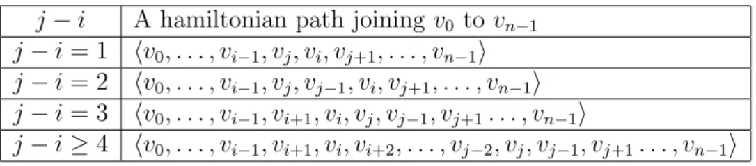
Table 1: Case 3.2 in Theorem 5.

j − i A hamiltonian path joining v₀ to v_n−1 j − i = 1 hv₀, . . . , v_i−1, v_j, v_i, v_j+1, . . . , v_n−1i j − i = 2 hv₀, . . . , v_i−1, v_j, v_j−1, v_i, v_j+1, . . . , v_n−1i j − i = 3 hv₀, . . . , v_i−1, v_i+1, v_i, v_j, v_j−1, v_j+1. . . , v_n−1i

j − i ≥ 4 hv₀, . . . , v_i−1, v_i+1, v_i, v_i+2, . . . , v_j−2, v_j, v_j−1, v_j+1. . . , v_n−1i

Lemma 1. [2] Let n ≥ 3. There exists a hamiltonian path with endvertices v₀ and v₁ in P_n².

The following two lemmas are obvious.

Lemma 2. Let n ≥ 5. Then P_n² − S has a hamiltonian path with endvertices v₀ and v_n−1 for S ⊂ (V (P_n²) − {v₀, v_n−1}) ∪ E(P_n²) with |S| ≤ 1.

Lemma 3. Let n ≥ 4. Then P_n³ − S has a hamiltonian path with endvertices v₀and v_n−1 for S ⊂ (V (P_n³) − {v₀, v_n−1}) with |S| ≤ 2.

Theorem 5. Let n ≥ 6 and S ⊂ E(P_n³) with

|S| ≤ 2. Then there exists a hamiltonian path of P_n³− S with endvertices v₀ and v_n−1. Proof. It suffices to prove this theorem for that S ⊂ E(P_n³) with |S| = 2. Let E(P_n³) = A₁∪ A₂∪ A₃, where A_l= {(v_i, v_j) ∈ E(P_n³)|j = i + l}. Let S_i = S ∩ A_i for i = 1, 2, 3. If |S3| > 0, by Lemma 2, there ex- ists a hamiltonian path of P_n³−S with endver- tices v₀ and v_n−1. Thus, we assume |S₃| = 0.

There are three cases:

Case 1. |S₁| = 0. hv₀, v₁, . . . , v_n−1i is the required path.

Case 2. |S1| = 1. Note that |S2| = 1.

Assume that S₁ = {(v_i, v_i+1)}, where 0 ≤ i ≤ bⁿ⁻²₂ c. Therefore, hv₀, v₃, v₄, v₁, v₂, v₅i is the required path when n = 6 and i = 2; hv₀, . . . , v_i, v_i+3, v_i+2, v_i+1, v_i+4, . . . , v_n−1i is the required path if otherwise.

Case 3. |S1| = 2. We assume that S1 = {(v_i−1, v_i), (v_j, v_j+1)}, where 1 ≤ i ≤ j ≤ n − 2.

Case 3.1. i = j. Without loss of generality, we assume that 1 ≤ i ≤ bⁿ⁻¹₂ c. Then hv₀, . . . , v_i−1, v_i+1, v_i+2, v_i, v_i+3, . . . , v_n−1i is the re- quired path.

Case 3.2. i < j. The hamiltonian paths join- ing v₀ to v_n−1 are listed in Table 1.

Corollary 1. Let n ≥ 6. Then P_n³ − S has a hamiltonian path with endvertices v0 and v_n−1 for S ⊂ (V (P_n³) − {v₀, v_n−1}) ∪ E(P_n³) with |S| ≤ 2.

Proof. According to Lemma 3 and Theo- rem 5, it suffices to consider the case when S is composed of one vertex and one edge. Let S = {v, e}, where v ∈ (V (P_n³) − {v₀, v_n−1}) and e ∈ E(P_n³) is not incident to v. Note that P_n−1² is a subgraph of P_n³ − {v}. Therefore, by Lemma 2, P_n³ − {v, e} has a hamiltonian path with endvertices v₀ and v_n−1.

3 The 4-Hamiltonicity of G(n, 4)

Theorem 6. The graph G(n, 4) is 4-hamilto- nian for n ≥ 9.

Proof. Let S ⊂ V (G(n, 4)) ∪ E(G(n, 4)) with

|S| = 4. We want to prove that there exists a hamiltonian cycle in G(n, 4) − S. According to Theorem 1, G(n, 4) − S is hamiltonian for S ⊂ V (G(n, 4)) or S ⊂ E(G(n, 4)). Hence it suffices to consider the remaining three cases.

Case 1. S is composed of three vertices and one edge. Without loss of generality, we assume that the three removed vertices are

v₀, v_i, and v_j with 0 < i < j and i ≤ j − i

≤ n − j.

Case 1.1. j ≥ 3. Since n − 2 ≥ 7, G(n − 2, 2) is a subgraph of G(n, 4) − {v₀, v_j}. By Theorem 3, G(n − 2, 2) is a 2-hamiltonian graph. Thus G(n, 4) − S is hamiltonian.

Case 1.2. j = 2. Note that i = 1. The remaining graph after the removal of the vertices v₀, v₁, and v₂ of G(n, 4) is isomorphic to the graph P_n−3³ . By Theorem 4, P_n−3³ is 1-edge hamiltonian. Thus G(n, 4) − S is hamiltonian.

Case 2. S is composed of two vertices and two edges. Without loss of generality, we assume that {v₀, v_i} ∈ S, where 1 ≤ i ≤ bⁿ₂c.

Case 2.1. i ≥ 3. Note that G(n − 2, 2) is a subgraph of G(n, 4) − {v₀, v_i}. Since n − 2 ≥ 7 and by Theorem 3, G(n − 2, 2) is a 2-hamiltonian graph. Thus G(n, 4) − S is hamiltonian.

v

v

v

v

v

v

v

v

v

Figure 2: G(n, 4) − {v₀, v₂}.

Case 2.2. i = 2. The remaining graph after the removal of v0 and v2of G(n, 4) is depicted in Figure 2. Let G⁰ be the subgraph of G induced by {v₃, v₄, . . . , v_n−1}. Obviously, G⁰ is isomorphic to P_n−3³ .

Case 2.2.1. |{(v₁, v₃), (v₁, v_n−1)} ∩ S| = 0. By Theorem 5, G⁰ has a hamiltonian path Q1

with endvertices v₃ and v_n−1 after removing any two edges. Thus, hv₃, Q₁, v_n−1, v₁, v₃i is

the hamiltonian cycle of G(n, 4) − S.

Case 2.2.2. |{(v₁, v₃), (v₁, v_n−1)} ∩ S| = 2.

hv1, v4, v3, v5, . . . , vn−3, vn−1, vn−2, v1i is the hamiltonian cycle of G(n, 4) − S.

Case 2.2.3. |{(v1, v3), (v1, vn−1)} ∩ S| = 1.

Without loss of generality, we assume that (v₁, v_n−1) ∈ S. Suppose that {(v₁, v_n−2), (vn−1, vn−2)} ∩ S = ∅. By Corollary 1, G⁰− {v_n−2} has a hamiltonian path Q₂ with endvertices v₃ and v_n−1 after removing any one edge. Thus hv3, Q2, vn−1, vn−2, v1, v3i is the hamiltonian cycle of G(n, 4)−S. Suppose that (v₁, v_n−2) ∈ S. P_n−3² is the subgraph of G⁰. By Lemma 1, there exists a hamiltonian path Q₃ of G⁰ with endvertices v₃ and v₄. Thus hv₄, v₁, v₃, Q₃, v₄i is the required cycle.

Suppose that (vn−1, vn−2) ∈ S, hv1, v3, . . . , v_n−4, v_n−1, v_n−3, v_n−2, v₁i is the required cycle.

v

v

v

v

v

v

v

v

Figure 3: G(n, 4) − {v₀, v₁}.

Case 2.3. i = 1. The remaining graph after the removal of v₀ and v₁ of G(n, 4) is depicted in Figure 3. Suppose that (v_n−1, v₂) ∈ S.

G(n, 4) − {v0, v1, (vn−1, v2)} is isomorphic to P_n−2³ which is 1-edge hamiltonian. Hence, the remaining graph after removing any one edge from G(n, 4) − {v0, v1, (vn−1, v2)}

contains a hamiltonian cycle. Suppose that (v_n−1, v₂) /∈ S. Since the graph G(n, 4) − {v₀, v1, (vn−1, v2)} is isomorphic to P_n−2³ , it has a hamiltonian path Q₄ with endvertices v₂ and v_n−1 after removing any two edges. Thus,

hv₂, Q₄, v_n−1, v₂i is the required cycle.

v

v

v

v

v

v

v

v

Figure 4: G⁰⁰= G(n, 4) − {v_n−1}.

Case 3. S is composed of one vertex and three edges. Without loss of generality, we assume that v_n−1 ∈ S. The graph G(n, 4) − {vn−1} is depicted in Figure 4. Let G⁰⁰ = G(n, 4)−{v_n−1}. In this case, all the addition and subtraction are carried with modulo n − 1. Let E(G⁰⁰) = A1 ∪ A2 ∪ A3, where Al = {(v_i, v_j) ∈ E(G⁰⁰)|j = i + l}. Let S_i = S ∩ A_i for i = 1, 2, 3.

Suppose that S₃ 6= ∅. For any edge e ∈ S₃, G(n − 1, 2) is a subgraph of G⁰⁰ − {e}. By Theorem 3, there exists a hamiltonian cycle after removing any two edges. Now, we as- sume that S₃ = ∅. We consider the remaining cases in the following:

Case 3.1. |S₂| = 3. Cycle hv₀, v₁, . . . , v_n−2, v₀i is the required cycle.

Case 3.2. |S₁| = 1. Note that |S₂| = 2.

If (v_n−2, v₀) /∈ S₁, without loss of general- ity, we suppose that S₁ = {(v_i, v_i+1)}, where 0 ≤ i ≤ bⁿ⁻³₂ c. Thus hv₀, . . . , v_i, v_i+3, v_i+2, v_i+1, v_i+4, . . . , v_n−2, v₀i is a hamiltonian cycle of G(n, 4) − S. Next, we consider the case that (v_n−2, v₀) ∈ S₁ in the following two sub- cases.

Case 3.2.1. |{(v_n−3, v₀), (v_n−2, v₁)} ∩ S₂| ≥ 1. Note that G⁰⁰ − {(vn−2, v0), (vn−3, v0), (v_n−2, v₁)} is isomorphic to P_n−1³ and P_n−1³ is 1-edge hamiltonian. Thus G(n, 4) − S is

hamiltonian.

Case 3.2.2. |{(v_n−3, v₀), (v_n−2, v₁)} ∩ S₂| = 0.

If |{(v₀, v₂), (v_n−4, v_n−2)} ∩ S₂| = 2, then hv₀, v₃, v₂, v₄, . . . , v_n−2, v₁, v₀i is the required cycle. Otherwise, |{(v₀, v₂), (v_n−4, v_n−2)} ∩ S₂| ≤ 1. Without loss of generality, we as- sume that (v₀, v₂) /∈ S₂. Thus hv₀, v₂, . . . , v_n−2, v₁, v₀i is the required cycle.

Case 3.3. |S₁| = 2. Note that |S₂| = 1.

Case 3.3.1. The two edges in S₁ are adjacent.

Assume that S₁ = {(v_i−1, v_i), (v_i, v_i+1)}, where 0 ≤ i ≤ bⁿ⁻²₂ c. hvi−1, vi+1, vi+2, vi, v_i+3, . . . , v_i−1i is the required cycle if

|{(v_i−1, v_i+1), (v_i, v_i+2)} ∩ S₂| = 0; hv_i−3, v_i−1, vi−2, vi, vi+3, vi+2, vi+1, vi+4, . . . , vi−3i is the required cycle if otherwise.

Case 3.3.2. The two edges in S1 are not ad- jacent.

Case 3.3.2.1. (vn−2, v0) /∈ S1. Without loss of generality, we assume that S₁ = {(v_i−1, v_i), (v_j, v_j+1) | 1 ≤ i < j ≤ n − 3}.

When j − i = 4, hvi−1, vi+1, vi, vj−1, vj, v_j−2, v_j+1, . . . , v_i−1i is the required cycle if

|{(v_i−1, v_i+1), (v_j−2, v_j)} ∩S₂| = 0; hv_i−1, v_i+2, vi, vi+1, vj, vj−1, vj+1, . . . , vi−1i is the required cycle if otherwise. When j − i ≥ 1 and j − i 6= 4, the corresponding hamiltonian cycles listed in Table 2. Note that when j − i = 1, we assume that 1 ≤ i ≤ bⁿ⁻³₂ c.

Case 3.3.2.2. (vn−2, v0) ∈ S1. Without loss of generality, we assume that the other edge in S₁ is (v_i, v_i+1), where 1 ≤ i ≤ bⁿ⁻³₂ c. When i = 1, hv0, v2, . . . , vn−2, v1, v0i is the required cycle if |{(v_n−2, v₁), (v₀, v₂)} ∩ S₂| = 0, and hv₀, v₁, v₃, v₂, v₄, . . . , v_n−4, v_n−2, v_n−3, v₀i is the required cycle if otherwise. When 2 ≤ i ≤ bⁿ⁻³₂ c, hv₀, v₂, . . . , v_i, v_i+3, v_i+2, v_i+1, v_i+4, . . . , v_n−2, v₁, v₀i is the required cycle if |{(vn−2, v1), (v0, v2)} ∩ S2| = 0; hv0, . . . , v_i−2, v_i+1, v_i−1, v_i, v_i+2, . . . , v_n−4, v_n−2, v_n−3, v₀i is the required cycle if otherwise.

Table 2: Case 3.3.2.1 in Theorem 6.

j − i A hamiltonian cycle of G(n, 4) − S j − i = 1 hv_i−1, v_j+1, v_j+2, v_i, v_j, v_j+3, . . . , v_i−1i j − i = 2 hv_i−1, v_j, v_j−1, v_i, v_j+1, . . . , v_i−1i j − i = 3 hv_i−1, v_i+2, v_j, v_i, v_i+1, v_j+1. . . , v_i−1i

j − i = 5 hv_i−1, v_i+2, v_j, v_j−1, v_i+1, v_i, v_i+3, v_j+1, . . . , v_i−1i

j − i ≥ 6 hvi−1, vi+2, vi+1, vi, vi+3, . . . , vj−3, vj, vj−1, vj−2, vj+1, . . . , vi−1i

Case 3.4. |S₁| = 3.

Case 3.4.1. |V (G⁰⁰)| is odd. hv1, v3, v5, . . . , v_n−5, v_n−3, v₀ v₂, v₄,. . . , v_n−4, v_n−2, v₁i is the required cycle.

Case 3.4.2. |V (G⁰⁰)| is even. Since n ≥ 9 and |S₁| = 3, there exists an index i such that {(v_i, v_i+1), (v_i+2, v_i+3)} ∩ S₁ = ∅.

Thus, hvi+2, vi+4, vi+6, . . . , vi−4, vi−2, vi, vi+1, v_i−1, v_i−3, v_i−5, . . . , v_i+5, v_i+3, v_i+2i is the re- quired cycle.

References

[1] T. Y. Sung, T. Y. Ho, C. P. Chang and L.

H. Hsu, “Optimal k-Fault-Tolerant Net- works for Token Rings,” Journal of Infor- mation Science and Engineering, Vol. 16, pp.381-390, 2000.

[2] M. Paoli, W. W. Wong and C. K. Wong,

“Minimum k-Hamiltonian Graphs, II,”

Journal of Graph Theory, Vol. 10, pp.79- 95, 1986.

[3] W. W. Wong and C. K. Wong, “Mini- mum k-Hamiltonian Graphs,” Journal of Graph Theory, Vol. 8, pp.155-165, 1984.

[4] M. Paoli, “Powers of Connected Graphs and Hamiltonicity,” Discrete Mathemat- ics, Vol. 52, No.1, pp.91-99, 2002.

[5] G. Chartrand and S. F. Kapoor, “On Hamiltonian Properties of Powers of Spe- cial Hamiltonian Graphs,” Colloquium Mathematicum, Vol. 29, pp.113-117,1974.