國立臺灣大學理學院物理學系 碩士論文
Department of Physics College of Science
National Taiwan University Master Thesis
應用螢光顯微術比較分析兩肺腺癌細胞株 CL1-0 及 CL1-5 細胞核染色質
Comparative analysis of nucleus chromosome of lung
adenocarcinoma cell lines, CL1-0 and CL1-5, by fluorescence microscopy
傅學聖 Xue-Sheng Fu
指導教授:董成淵 博士
Advisor: Chen-Yuan Dong, Ph.D.
中華民國 105 年 7 月
Abstract
Lung cancer is the most lethal cancer. In Taiwan, the mortality rate of lung cancer ranks first among the cancer-related mortality rate in recent years. To reduce the morality, the early detection of the lung cancer may help the patient get the proper treatment in time. The DNA content abnormality is one of the characteristics which are observed in the tumor cells. Some researches show the potential prognostic value of it. In this thesis, to find the relation between invasive ability and DNA content abnormality, we use the two lung adenocarcinoma cell lines, CL1-0 and CL-5 which have different invasive ability and stain their nuclei with DAPI. By the fluorescence microscopy technique, quantify the DNA content of nuclei with the fluorescence and get nuclei DNA content distribution histogram. From the nuclei DNA content data, we find that the cell line with higher invasive ability has larger DNA content abnormality and the standard deviation of the DNA content of the cells may have potential to be the invasive ability index.
Keywords: lung adenocarcinoma, CL1-0, CL1-5, two-photon microscopy, DAPI, nucleus, DNA content abnormality
摘要
在所有癌症中肺癌是最致命的一種,近幾年在臺灣肺癌時常居於癌症十大死因之首。為了降 低肺癌的死亡率,在肺癌早期時發現能幫助病人即時的得到適當的治療。在腫瘤細胞中的 DNA 含量異常是一個被觀察到的特徵,有些研究顯示這有用來預測病情的潛力。在本論文中
為了找出轉移能力和DNA 含量異常的關係,使用了兩種不同轉移能力的肺腺癌細胞株 CL1-0
及CL1-5 並使用 DAPI 這種染劑對細胞核染色。透過螢光顯微術,將 DNA 含量以螢光訊號量
化,並得到細胞核DNA 含量的分布圖。從這些 DNA 含量的資料發現,DNA 含量異常越顯
著的細胞株,其轉移能力亦越強。此外,計算一群細胞的DNA 含量的標準差,有做為轉移
能力指標的潛力。
關鍵字: 肺腺癌、CL1-0、CL1-5、雙光子顯微術、DAPI、細胞核、DNA 含量異常
Contents
Abstract………...i
中文摘要……….ii
Contents………..iii
List of Figures and table...……….iv
Chapter 1 Introduction……….1
Chapter 2 Basic Principles………3
2.1 Two-photon excitation………..3
2.2 Principles of optical microscopy………...11
2.2.1 Mode locking………11
2.2.2 Light intensity distribution near focus………..13
2.2.3 Resolution……….16
Chapter 3 Materials and Methods……….19
3.1 Laser and microscope……….19
3.2 Stain………... 21
3.3 Cell line CL1………..23
3.4 Preparation for the sample………..24
3.5 Setting of microscope and operation procedure...25
Chapter 4 Results and discussion………...26
4.1 Image processing………...26
4.2 z-stack summation image………...28
4.3 Comparison of CL1-0 and CL1-5………..29
References……….33
Figure Catalog
Figure 1.1 the ranking and population of different cancer cause death in 2014………2
Figure 2.1.1 State m as the density of states described by ρ(ωmg)………6
Figure 2.1.2 two photon absorption process………...7
Figure 2.1.4 the contour of 𝐼(𝑟,𝑧) 𝐼𝑚𝑎𝑥………....10
Figure 2.1.5 the contour of (𝐼(𝑟,𝑧) 𝐼𝑚𝑎𝑥)2………...10
Figure 2.2.1 (a) Mode-locked laser with constant mode phase; (b) laser with random mode phase……….13
Figure 2.2.2 the incident ray converged by the lens………..14
Figure 2.2.3 the spherical wave converging to O………..14
Figure 2.2.4 the objective with NA=0.75………..18
Figure 3.1.1 Laser and microscope system………20
Figure 3.2.1 chemical formula of DAPI………22
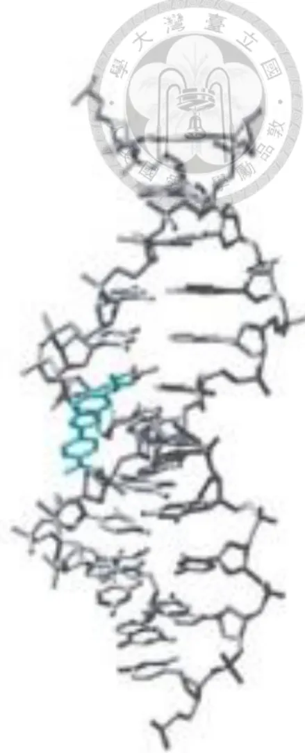
Figure 3.2.2 DAPI bind to DNA ………...22
Figure 3.2.3 Excitation and emission spectrum of DAPI………..22
Figure 3.3.1 the method of cell line selection………23
Figure 3.4.1 the method to stain DAPI………..25
Figure 3.4.2 complete sample………25
Figure 4.1.1 Image processing and data acquisition………..27
Figure 4.2.1 integrated intensity of cells in z-stack summation image – in highest intensity single layer image………...28
Figure 4.3.1 Integrated intensity distribution histogram of CL1-0 and CL1-5……….30
Figure 4.3.2 area distribution histogram of CL1-0 and CL1-5………..31
Figure 4.3.3 integrated intensity – area diagram of CL1-0 and CL1-5………31 Figure 4.3.4 Nucleus average density distribution histogram of CL1-0 and CL1-5………32
Table Catalog
Table 4.4.1 Statistical value of some quantities of CL1-0 and CL1-5………..32
Introduction
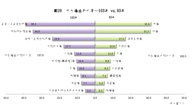
Lung cancer is the second most common cancer in both men and women, and the most lethal among all kinds of cancers[3]. In Taiwan, the mortality rate of lung cancer is 39.2 and ranks first among the cancer-related mortality rate, 197.0 in 2014[1]. The five-year survival rate is about 17% in the United States[2].
Lung cancer can be classified into two main types, non-small cell lung cancer (NSCLC) and small cell lung cancer (SCLC). There are about 80% to 85% of lung cancers which are NSCLC and 10%
to 15% which are SCLC. NSCLC can be further divided into several subtypes which start from different types of lung cells. The subtypes are adenocarcinoma, squamous cell (epidermoid)
carcinoma, large cell (undifferentiated) carcinoma, and other subtypes which is much less common.
Among the subtypes, adenocarcinoma is the most common that about 40% of lung cancers are adenocarcinomas. Adenocarcinoma occurs mainly in current or former smokers, but it is also the most common type of lung cancer seen in non-smokers[3].
The early detection of lung cancer is challengeable. The symptoms usually do not appear until the disease is at an advanced stage. However, there are still some methods that have potential to achieve early detection. In clinical, low-dose computed tomography (LDCT) is a technique to find lung cancer before the symptoms appear. And it has been shown by a study that the screening can lower the mortality from lung cancer[4].
DNA content abnormality or the common term of aneuploidy probably reflects a high genotypic instability in lung cancer. There are some reports showing that DNA content abnormality measured by flow cytometry might be a prognostic factor[5][6], however the conflict results also exists[7].
Despite the heterogeneity across the studies, there is a meta-analysis conclude that patients who benefit from a surgical resection for NSCLC with aneuploid DNA content have a higher risk of death. [8].
5.1 5.3 7.1
8.3 8.8
11.0 12.0
17.2
31.2 31.6
5.5 7.7 8.1 10.0 10.4 11.6 17.7 23.9 34.9
39.2
胰臟癌 食道癌
攝護腺癌 子宮頸癌
口腔癌 胃癌
女性乳癌 結腸直腸癌
肝癌 肺癌
子宮頸及部位未明示子宮癌 食道癌 胰臟癌 胃癌 前列腺(攝護腺)癌
口腔癌 女性乳房癌 結腸、直腸和肛門癌 肝和肝內膽管癌
氣管、支氣管和肺癌
160.5 197.0
50.0 40.0 30.0 20.0 10.0 0.0 10.0 20.0 30.0 40.0 50.0
103年 93年
圖20 十大癌症死亡率--103年 vs.93年
所有癌症死因死亡率 所有癌症死因死亡率
每十萬人口
In this thesis, the method to measure DNA content of cells is imaging by fluorescence microscopy.
By comparing the two cell lines CL1-0 and CL1-5 which have different invasive ability, try to find the judgment of invasive ability with DNA content abnormality.
Figure 1.1 the ranking and population of different cancer cause death in 2014
Chapter 2. Basic principles
2.1 Two –Photon Excitation[9]
To understand two-photon excitation, time-dependent Schrödinger equation is used to calculate the photon absorption rate. By perturbation theory, we derive the standard result of the single-photon absorption rate and generalize the result to higher order which represent the multiphoton absorption processes.
We assume that the atomic wave function |𝜓(𝒓, 𝑡)〉obeys the time-dependent Schrödinger equation
𝑖ħ 𝜕
𝜕𝑡│𝜓(𝑡)〉 = 𝐻̂│𝜓(𝑡)〉, (2.1.1)
where the Hamiltonian 𝐻̂ is represented
𝐻̂ = 𝐻̂0+ 𝑉̂(𝑡), (2.1.2)
Here 𝐻̂0 is the time-independent Hamiltonian for free atom and
𝑉̂ = −𝜇̂𝐸̃(𝑡), (2.1.3)
where 𝜇̂ = −e𝑟̂, is the interaction energy with the electrified of the incoming light. For simplicity we take the monochromatic wave of which the electric field takes the form
𝐸̃(𝑡) = 𝐸𝑒−𝑖𝜔𝑡+ 𝐸∗𝑒𝑖𝜔𝑡 . (2.1.4)
We assume the solutions of 𝐻̂0 are known as the eigenstates │𝑛〉and eigenvalues 𝐸𝑛, then the time dependent wave, │𝜓(𝑡)〉, can be represented as
│𝜓(𝑡)〉 = ∑ 𝑎𝑛(𝑡)𝑒−𝑖𝜔𝑛𝑡│𝑛〉
𝑛
. (2.1.5)
where 𝜔𝑛 = 𝐸𝑛/ħ. Substitute Eq. (2.1.5) into Eq. (2.1.1), then the equation becomes
𝑖ħ ∑[𝑎𝑛̇ (𝑡)−𝑖𝜔𝑛𝑎𝑛(𝑡)]𝑒−𝑖𝜔𝑛𝑡│𝑛〉
𝑛
= (𝐻̂0+ 𝑉̂) ∑ 𝑎𝑛(𝑡)𝑒−𝑖𝜔𝑛𝑡│𝑛〉
𝑛
(2.1.6)
The two terms corresponding to the free atom solution can be canceled. Therefore we get 𝑖ħ ∑ 𝑎𝑛̇ (𝑡)𝑒−𝑖𝜔𝑛𝑡│𝑛〉
𝑛
= 𝑉̂ ∑ 𝑎𝑛(𝑡)𝑒−𝑖𝜔𝑛𝑡│𝑛〉
𝑛
. (2.1.7)
To simplify the Eq. (2.1.7), we use the orthonormality condition,〈m│𝑛〉 = δ
𝑚𝑛. multiply
〈𝑚│ on both sides of equation. We obtain
𝑖ħ𝑑𝑎𝑚
𝑑𝑡 = ∑ 𝑎𝑛(𝑡)𝑒−𝑖𝜔𝑛𝑚𝑡𝑉𝑚𝑛
𝑛
(2.1.8)
where 𝑉𝑚𝑛 = 〈m│𝑉̂│n〉and 𝜔𝑛𝑚 = 𝜔𝑛 − 𝜔𝑚.Using perturbation techniques, we introduce a parameter λ, replace 𝑉𝑚𝑛 by λ𝑉𝑚𝑛 and expand 𝑎𝑛(t) in powers of the interaction as
𝑎𝑚(t) = 𝑎𝑚(0)(𝑡) + λ𝑎𝑚(1)(𝑡) + λ2𝑎𝑚(2)(𝑡) + ⋯ . (2.1.9)
By equating the powers of λ on both sides of Eq. (2.1.8), we get 𝑑𝑎𝑚(𝑁)
𝑑𝑡 = (𝑖ħ)−1∑ 𝑎𝑛(𝑁−1)𝑒−𝑖𝜔𝑛𝑚𝑡𝑉𝑚𝑛
𝑛
. 𝑁 = 1,2,3, … (2.1.10)
Assume that the atom is originally in the state g without the applied laser field so that
𝑎𝑔(0)(𝑡) = 1, and 𝑎𝑛(0)(𝑡) = 0 for n ≠ g . (2.1.11)
for all time t.
By using Eq. (2.1.3) and Eq. (2.1.4), represent 𝑉𝑚𝑛 as −𝜇𝑚𝑛 (𝐸𝑒−𝑖𝜔𝑡+ 𝐸∗𝑒𝑖𝜔𝑡) and consider the first order of Eq. (2.1.10) which is
𝑑𝑎𝑚(1)
𝑑𝑡 = −(𝑖ħ)−1𝜇𝑚𝑔 [𝐸𝑒𝑖(𝜔𝑚𝑔−𝜔)𝑡+ 𝐸∗𝑒𝑖(𝜔𝑚𝑔+𝜔)𝑡]. (2.1.12) The equation above can be integrated to solve 𝑎𝑚(1) as
𝑎𝑚(1)(𝑡) = −(𝑖ħ)−1𝜇𝑚𝑔 ∫ 𝑑𝑡′
𝑡 0
[𝐸𝑒𝑖(𝜔𝑚𝑔−𝜔)𝑡′+ 𝐸∗𝑒𝑖(𝜔𝑚𝑔+𝜔)𝑡′]
= 𝜇𝑚𝑔𝐸
ħ(𝜔𝑚𝑔− 𝜔)[𝑒𝑖(𝜔𝑚𝑔−𝜔)𝑡− 1] + 𝜇𝑚𝑔𝐸∗
ħ(𝜔𝑚𝑔+ 𝜔)[𝑒𝑖(𝜔𝑚𝑔+𝜔)𝑡− 1]
(2.1.13)
The first term of Eq. (2.1.13) represents the process of the one photon absorption and the second term correspond to the one photon emission. Since our interest is photon absorption, we drop the second term. The probability 𝑝𝑚(1) that the atom is in state m at time t is given by
𝑝𝑚(1)= |𝑎𝑚(1)(𝑡)|2 = |𝜇𝑚𝑔𝐸|2 ħ2
|𝑒𝑖(𝜔𝑚𝑔−𝜔)𝑡− 1|2 (𝜔𝑚𝑔− 𝜔)2
=|𝜇𝑚𝑔𝐸|2 ħ2
4 sin2[(𝜔𝑚𝑔− 𝜔) 𝑡/2]
(𝜔𝑚𝑔− 𝜔)2 =|𝜇𝑚𝑔𝐸|2 ħ2 𝑓(𝑡)
(2.1.14)
where
𝑓(𝑡) =4 sin2[(𝜔𝑚𝑔− 𝜔) 𝑡/2]
(𝜔𝑚𝑔− 𝜔)2 𝑎𝑛𝑑 lim
𝑡→∞𝑓(𝑡) = 2πtδ(ωmg− ω) (2.1.15) With the Eq. (2.1.14), the Eq. (2.1.15) at large t becomes
𝑝𝑚(1) =|𝜇𝑚𝑔𝐸|2t
ħ2 2πδ(ωmg− ω). (2.1.16)
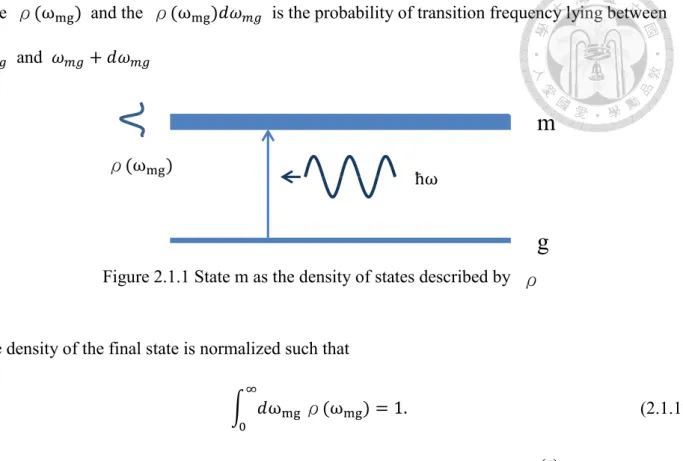
The infinity of the delta function which appears in Eq. (2.1.16) is somewhat unphysical in the real situation. To deal with that, we should consider that the final state m would spread into a density of
state ρ(ωmg) and the ρ(ωmg)𝑑𝜔𝑚𝑔 is the probability of transition frequency lying between 𝜔𝑚𝑔 and 𝜔𝑚𝑔+ 𝑑𝜔𝑚𝑔
The density of the final state is normalized such that
∫ 𝑑ωmg
∞ 0
ρ(ωmg) = 1. (2.1.17)
Using the density function of continuous state m, the transition probability 𝑝𝑚(1) that the atom transit from state g to state m is given by
𝑝𝑚(1) =2𝜋|𝜇𝑚𝑔𝐸|2𝑡
ħ2 ∫ 𝑑ωmg
∞ 0
ρ(ωmg)𝛿(𝜔𝑚𝑔 − 𝜔)
= 2𝜋|𝜇𝑚𝑔𝐸|2𝑡
ħ2 ρ(ωmg= 𝜔).
(2.1.18)
The transition probability above is linearly increase with the time, hence the transition can rate can be defined as
𝑅𝑚𝑔(1) =𝑝𝑚(1)
𝑡 = 2𝜋|𝜇𝑚𝑔𝐸|2
ħ2 ρ(ωmg = 𝜔). (2.1.19)
Now we get the result of linear absorption, the transition rate of the single photon absorption with the applied laser field of which the frequency is 𝜔.
Figure 2.1.1 State m as the density of states described by
m
g
ρ(ωmg)
ħω
ρ
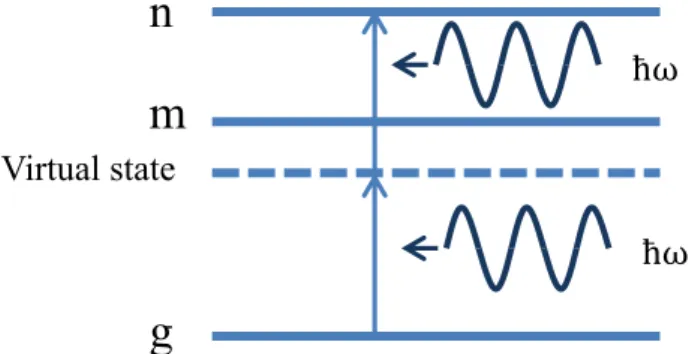
Next we will calculate the second order term of the Eq. (2.1.10) which describes the two-photon absorption process (Fig 2.1.2).
As the previous discussion, we only keep the term that represent absorption process in 𝑉𝑛𝑔 which becomes 𝑉𝑛𝑔 = −𝜇𝑛𝑔𝐸𝑒−𝑖𝜔𝑡. With the Eq. (2.1.13), the second order term of the Eq. (2.1.10) can be written as
𝑑𝑎𝑛(2)
𝑑𝑡 = (𝑖ħ)−1∑ 𝑎𝑚(1)𝑒−𝑖𝜔𝑚𝑛𝑡𝑉𝑛𝑚
𝑚
= −(𝑖ħ)−1∑ 𝜇𝑛𝑔𝜇𝑚𝑔𝐸2
ħ(𝜔𝑚𝑔− 𝜔)𝑒𝑖(𝜔𝑛𝑔−2𝜔)𝑡.
𝑚
(2.1.20)
Integrate Eq. (2.1.20)
= ∑ 𝜇𝑛𝑔𝜇𝑚𝑔𝐸2
ħ2(𝜔𝑚𝑔 − 𝜔)[𝑒𝑖(𝜔𝑛𝑔−2𝜔)𝑡− 1 𝜔𝑛𝑔− 2𝜔 ]
𝑚
.. (2.1.21)
The probability of the atom being state n at time t is given by
𝑝𝑚(2)= |𝑎𝑛(2)|2 = |∑ 𝜇𝑛𝑔𝜇𝑚𝑔𝐸2 ħ2(𝜔𝑚𝑔− 𝜔)
𝑚
|
2
|𝑒𝑖(𝜔𝑛𝑔−2𝜔)𝑡− 1 𝜔𝑛𝑔− 2𝜔 |
2
.. (2.1.22)
The last term of the Eq. (2.1.22) has the same form as the Eq. (2.1.14).
Virtual state
ħω
ħω
n m
g
Figure 2.1.2 two photon absorption process
While t → ∞, Eq. (2.1.22) would becomes
𝑝𝑛(2) = |𝑎𝑛(2)|2 = |∑ 𝜇𝑛𝑔𝜇𝑚𝑔𝐸2 ħ2(𝜔𝑚𝑔− 𝜔)
𝑚
|
2
2𝜋𝑡𝛿(𝜔𝑛𝑔− 𝜔). (2.1.23)
By the same argument, introduce the density of state n, ρ(ωng), again. we get
𝑝𝑛(2) = |∑ 𝜇𝑛𝑔𝜇𝑚𝑔𝐸2 ħ2(𝜔𝑚𝑔− 𝜔)
𝑚
|
2
2𝜋𝑡𝜌(𝜔𝑛𝑔= 2𝜔). (2.1.24)
Thus the transition rate of two photon absorption process is
𝑅𝑛𝑔(2) =𝑝𝑚(1)
𝑡 = |∑ 𝜇𝑛𝑔𝜇𝑚𝑔𝐸2 ħ2(𝜔𝑚𝑔 − 𝜔)
𝑚
|
2
2𝜋ρ(ωng= 2𝜔). (2.1.25)
From Eq. (2.1.19), the transition rate of the single photon absorption is proportional to |𝐸|2, the intensity of the excitation light source 𝐼. While the Eq. (2.1.25) shows that the transition rate of the two-photon absorption is proportional to |𝐸|4 , the square of the light source intensity 𝐼2. When the excitation light is focused by the objectives, the two photon excitation occurs only in the vicinity of the focal point. Since the fast decay of the term 𝐼2, outside the focal volume the intensity of the excitation light is not high enough for the two photon absorption. In contrast, the single photon absorption will happen in the excitation light cone as showed in Figure (2.1.3).
To better understand the excitation volume, we examine the spatial distribution of the laser intensity in the vicinity of the focal point of the beam. There are four equations below that we will use[10].
First we assume our laser beam is a Gaussian beam which propagates along z axis and is cylindrically symmetric about z axis. The intensity of the laser is given by
𝐼(𝑟, 𝑧) = 𝐼0(𝑧)𝑒
−2𝑟2
𝑤(𝑧)2. (2.1.26)
where 𝑟 is the distance from z axis, 𝐼0(𝑧) is the intensity along the z axis, and w(z) is the beam width along the z axis. The intensity is related to the power P per unit area by,
𝐼0(𝑧) = 2𝑃
𝜋𝑤(𝑧)2. (2.1.27)
The factor of two in equation above comes from the integration of Eq. (2.1.26) over all angles and from zero to infinity in 𝒓 to ensure the conservation of photon flux as the beam reshape. The beam radius is related to the focal location as,
𝑤(𝑧)2 = 𝑤02[1 + ( 𝜆𝑧
𝜋𝑤02)2] (2.1.28)
where 𝜆 is the wave length of the laser. 𝑤0 is the beam radius at the focal waist and it can be related to the system as
𝑤0 = 𝜆𝑓
𝜋𝑤𝐿 (2.1.29)
where 𝑤𝐿 is the beam radius at the system lens and 𝑓 is the focal length of the lens.
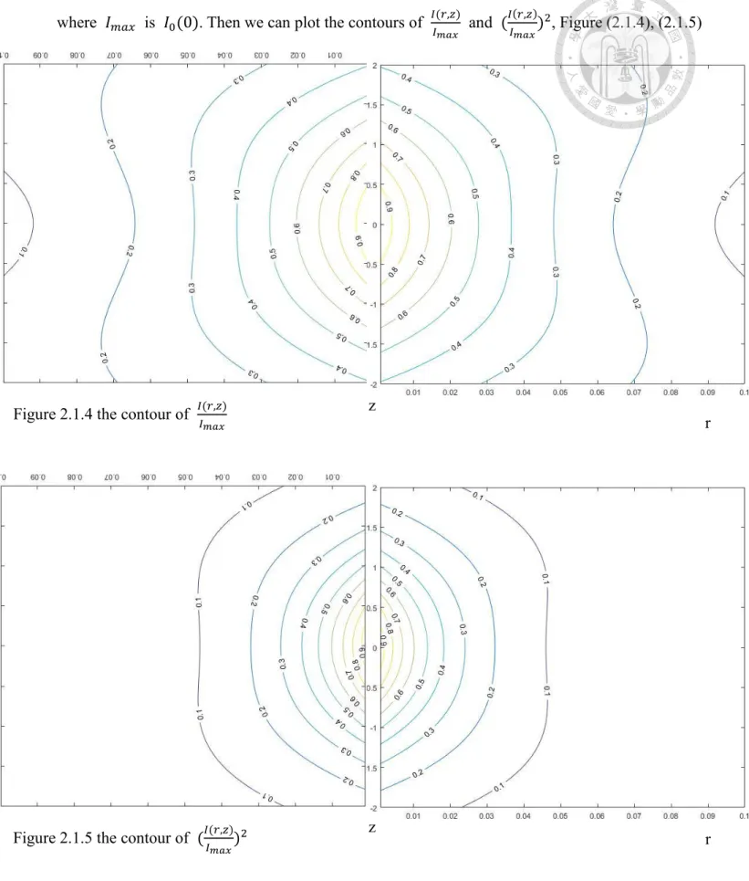
By combining the Eq. (2.1.26), Eq. (2.1.27) and (2.1.28), we get
𝐼(𝑟, 𝑧) 𝐼𝑚𝑎𝑥 =
𝑒𝑥𝑝(−2𝑟2/𝑤02[1 + ( 𝜆𝑧 𝜋𝑤02)2]) [1 + ( 𝜆𝑧
𝜋𝑤02)2]
(2.1.27)
z r
where 𝐼𝑚𝑎𝑥 is 𝐼0(0). Then we can plot the contours of 𝐼(𝑟,𝑧)
𝐼𝑚𝑎𝑥 and (𝐼(𝑟,𝑧)
𝐼𝑚𝑎𝑥)2, Figure (2.1.4), (2.1.5)
Figure 2.1.5 the contour of (𝐼(𝑟,𝑧)
𝐼𝑚𝑎𝑥)2 z r
Figure 2.1.4 the contour of 𝐼(𝑟,𝑧) r
𝐼𝑚𝑎𝑥
Due to the small excitation volume, the photo-bleaching is confined to the vicinity of the focal point in the two-photon excitation process. In addition, typically the two-photon microscopy uses the near infrared light which avoids the main absorption spectrum of biological tissue and hence will has better penetration to the deeper location of the tissue
2.2 principles of optical microscopy
2.2.1 mode-locking
To achieve two-photon excitation which is used with sensible biological sample, the ultrashort laser pulses are needed to provide enough intensity without the high pulse energy. Short pulses
generation requires broad bandwidth which means multiple longitudinal modes corresponding to the different wave length. However, random multimode is not enough for the pulse generation.
Mode-locking is required. In the following we will derive the time-domain characteristics of a multimode laser. The electric field of a multimode laser is
𝑒(𝑧, 𝑡) = 𝑅𝑒{∑ 𝐸𝑚𝑒𝑗(𝜔𝑚𝑡−𝑘𝑚𝑧+𝜑𝑚)
𝑚
} (2.2.1)
where
𝜔𝑚= 𝜔0+ 𝑚∆𝜔 = 𝜔0+2𝑚𝜋𝑐
𝐿 𝑎𝑛𝑑 𝑘𝑚 = 𝜔𝑚/𝑐 (2.2.2) With the Eq. (2.2.2), Eq. (2.2.1) can be rewritten as
𝑒(𝑧, 𝑡) = 𝑅𝑒 {𝑒𝑗𝜔0(𝑡−𝑧𝑐)∑ 𝐸𝑚𝑒𝑗[𝑚∆𝜔(𝑡−𝑧𝑐)+𝜑𝑚]
𝑚
}
= 𝑅𝑒 {𝑎(𝑡 − 𝑧/𝑐)𝑒𝑗𝜔0(𝑡−𝑧𝑐)}
(2.2.3)
where 𝑎 (𝑡 −𝑧
𝑐) = ∑ 𝐸𝑚 𝑚𝑒𝑗[𝑚∆𝜔(𝑡−𝑧𝑐)+𝜑𝑚].
Thus, the electric field can be regarded as a combination of a complex envelope function 𝑎 (𝑡 −𝑧
𝑐) and the optical carrier 𝑒𝑗𝜔0(𝑡−𝑧𝑐). In the laser cavity, both envelope and carrier functions travel at the speed of light and the time for the light taking one round trip around the resonator is
𝜏 =2𝑙 𝑐 = 2𝜋
∆𝜔 (2.2.4)
where 𝑙 is distance of the both sides of cavity and 𝜏 is also the time period of two pulses. To know more about the shape of the envelop we should deternine the mode amplitudes 𝐸𝑚 and phases 𝜑𝑚. For simplicity, we assume that there are N oscillating modes with equal amplitudes 𝐸0 and with the phases identically zero. The process that making the modes held with fixed relative phases is known as mode-locking. The Eq. (2.2.3) becomes
𝑒(𝑧, 𝑡) = 𝑅𝑒 {𝐸0𝑒𝑗𝜔0(𝑡−𝑧𝑐) ∑ 𝑒𝑗[𝑚∆𝜔(𝑡−𝑧𝑐)]
(𝑁−1)/2
−(𝑁−1)/2
} (2.2.5)
Substitute m′= m + (N − 1)/2
𝑒(𝑧, 𝑡) = 𝑅𝑒 {𝐸0𝑒𝑗𝜔0(𝑡−𝑧𝑐)−𝑗∆𝜔(𝑁−12 )(𝑡−𝑧𝑐)∑ 𝑒𝑗[𝑚∆𝜔(𝑡−𝑧𝑐)]
𝑁−1
0
}
= 𝑅𝑒 {𝐸0𝑒𝑗𝜔0(𝑡−𝑧𝑐)−𝑗∆𝜔(𝑁−12 )(𝑡−𝑧𝑐)1 − 𝑒𝑗[𝑁∆𝜔(𝑡−𝑧𝑐)]
1 − 𝑒𝑗∆𝜔(𝑡−𝑧𝑐) }
= 𝑅𝑒 {𝐸0𝑒𝑗𝜔0(𝑡−𝑧𝑐)sin (𝑁∆𝜔/2) (𝑡 −𝑧 𝑐)) sin (∆𝜔
2 ) (𝑡 − 𝑧 𝑐)
}
(2.2.6)
The laser intensity, I, averaged over an optical cycle, is proportional to |𝑒(𝑧, 𝑡)|2. At z=0, the intensity is
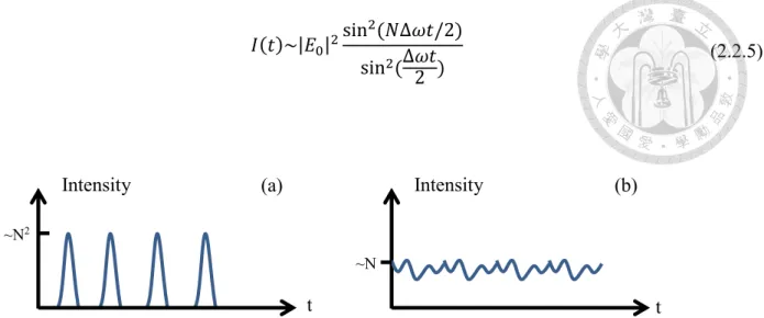
𝐼(𝑡)~|𝐸0|2sin 2(𝑁∆𝜔𝑡/2) sin2 (∆𝜔𝑡
2 )
(2.2.5)
The pulse duration is approximately determined by the number of modes, ∆𝑡 = 2π
N∆𝜔= 1/𝜈.
Equivalently, the pulse width is equal to the inverse of the laser bandwidth. The peak intensity is proportional to N2. Compare to the intensity of random mode phase laser which is proportional to N, the peak intensity has a factor 2 enhancement.
In the real situation, not only the mode phase is modulated, the mode amplitude would also be modulated during each round trip in the cavity. The pulse is shaped through the process. Modulation plays a key role in initiating and maintaining mode-locked laser operation.
2.2.2 Light intensity distribution near focus[11]
When the incoming ray focused by the lens, due to the diffraction of the light, the light cannot be totally converged to the focal point. The intensity distribution will appear in the vicinity of the focal point.
According to the Huygens-Fresnel principle, every point in the wavefront can be considered as an independent point source and propagate outward as a spherical wave. To get the intensity of a point,
t t
~N
~N2
Intensity Intensity Intensity
Figure 2.2.1 (a) Mode-locked laser with constant mode phase; (b) laser with random mode phase
(a) (b) a
one should sum the amplitude created by every source on the wavefront. In our situation which is an incident ray with a beam radius 𝒂 travelling parallel to the principal axis of the lens and then converging to the focal point, we assume that the converging process can be described as a
monochromatic spherical wave emerging from a circular aperture and converging toward the axial focal point showed as the following picture
The spherical wave propagating from a circular aperture with the diameter 2a (a>> 𝜆) and converge to the point O which is f distant from the center of aperture. The point P near the focus O is the position of observation specified by a vector 𝑅⃑ . We also assume that the radius of the aperture and
|𝑅⃑ | are both small compared to the radius of the wavefront W at the aperture and the amplitude of incident wavefront W is A/f. If a point Q is on the wavefront W, we determine that the distance
𝑅⃑
z 2a
W
C f
Q s
f𝑞
P z Figure 2.2.2 the incident ray converged by the lens
Figure 2.2.3 the spherical wave converging to O
O z
x z y
z
between Q and P is s and a vector f𝑞 is point from O to Q. By the Huygens-Fresnel principle, we can express the amplitude of the wave at point P as
𝑈(𝑃) = −𝑖 𝜆
𝐴𝑒−𝑖𝑘𝑓
𝑓 ∬𝑒𝑖𝑘𝑠
𝑠 𝑑𝑠. (2.2.6)
where 𝜆 is the wavelength of the wave. Consider the point P is near axis, hence approximately
s − f = −𝑞 ∙ 𝑅⃑ (2.2.7)
The Eq. (2.2.6) can be rewritten as
𝑈(𝑃) = −𝑖
𝜆𝐴 ∬ 𝑒−𝑖𝑘𝑞⃑ ∙𝑅⃑ 𝑑𝛺 (2.2.8)
where 𝑑𝛺 is the unit solid angle of the element Q. We take the origin of the Cartesian coordinate at O. The coordinates of points P and Q are (𝑥, 𝑦, 𝑧) and (𝜉, 𝜂, 𝜁). Using the polar coordinate on the x-y plane, rewrite the coordinates of P and Q as
{𝑥 = 𝑟 sin 𝜑 , 𝜉 = 𝑎𝜌sinθ
𝑦 = 𝑟 cos 𝜑 , 𝜂 = 𝑎𝜌𝑐𝑜𝑠𝜃 (2. 2.9)
𝜁 = −√𝑓2− 𝑎2𝜌2 = −𝑓[1 −1 2
𝑎2𝜌2
𝑓2 + ⋯ ] (2.2.10)
where a is the aperture radius and 𝜌 is a parameter which denote the distance of point Q to the center of the aperture in the unit of a. Furthermore, we get
𝑞 ∙ 𝑅⃑ =𝑥𝜉 + 𝑦𝜂 + 𝑧𝜁
𝑓 =𝑎𝜌 cos(𝜃 − 𝜑)
𝑓 − 𝑧[1 −1
2 𝑎2𝜌2
𝑓2 + ⋯ ] (2.2.11) 𝑑𝛺 =𝑑𝑠
𝑓2 =𝑎2𝜌𝑑𝜌𝑑𝜃
𝑓2 ,0 < 𝜌 < 1, 0 < 𝜃 < 2𝜋 (2.2.12) To simplify the calculation, we introduce two dimensionless parameter u and v defined as
𝑢 =2𝜋 𝜆 (𝑎
𝑓)2𝑧 ; 𝑣 =2𝜋 𝜆
𝑎
𝑓𝑟 (2.2.13)
Substituting u and v to express k𝑞 ∙ 𝑅⃑ , we get
𝑘𝑞 ∙ 𝑅⃑ = 𝑣𝜌 cos(𝜃 − 𝜑) − (𝑎 𝑓)
2
𝑢 +1
2𝑢𝜌2 (2.2.14)
The amplitude at the point P becomes
𝑈(𝑃) = − 𝑖𝑎2 𝜆𝑓2𝐴𝑒𝑖(
𝑎 𝑓)2𝑢
∫ ∫ 𝑒−𝑖[𝑣𝜌 cos(𝜃−𝜑)−+1 2𝑢𝜌2] 2𝜋
0 1
0
𝜌𝑑𝜌𝑑𝜃 (2.2.15)
Use the zero order Bessel function
𝐽0(𝑥) = 1
2𝜋∫ 𝑒𝑖𝑥𝑐𝑜𝑠(𝜗)
2𝜋
0
𝑑𝜗 = 𝐽0(−𝑥) (2.2.16)
Thus, we get
𝑈(𝑃) = −2𝜋𝑖𝑎2 𝜆𝑓2 𝐴𝑒𝑖(
𝑎 𝑓)2𝑢
∫ 𝐽0(𝑣𝜌)𝑒−2𝑖𝑢𝜌2
1
0
𝜌𝑑𝜌 (2.2.17)
Therefor we get the intensity distribution 𝐼(𝑢, 𝑣) near the focal point
𝐼(𝑢, 𝑣) = |𝑈(𝑃)|2 = |2 ∫ 𝐽0(𝑣𝜌)𝑒−2𝑖𝑢𝜌2
1
0
𝜌𝑑𝜌|
2
𝐼0 (2.2.18)
where 𝐼0 = (𝜋𝑎2
𝜆𝑓2𝐴)2
2.2.3 Resolution
The numerical aperture (NA) is one of the important properties of lens in microscopy and is defined by NA=sinθ where n is the index of refraction of the medium and θ is the maximal half-angle
of the cone of light that can enter or exit the lens(figure 2.2.4). The optical resolution is related to the numerical aperture and the light intensity distribution discussed in the previous section.
On the focal plane, z=0(u=0), the intensity distribution is
𝐼(0, 𝑣) = |2 ∫ 𝐽0(𝑣𝜌)
1
0
𝜌𝑑𝜌|
2
𝐼0 (2.2.19)
Use the relation of Bessel function, 𝑑
𝑑𝑥[𝑥𝑛+1𝐽𝑛+1(𝑥)] = 𝑥𝑛+1𝐽𝑛(𝑥) (2.2.20) The Eq. (2.) becomes
𝐼(0, 𝑣) = (2𝐽1(𝑣)
𝑣 )2𝐼0 (2.2.21)
When 𝑣 increase from 0, we find that the situation, 𝐽1(𝑣) = 0 , first appear at 𝑣 = 3.83, and
𝑣 =2𝜋 𝜆
𝑎
𝑓𝑟 = 3.83, → 2𝑟 ≈ 1.22𝜆𝑓
𝑎 (2.2.22)
Since 𝑎
𝑓≈ NA, the diameter D of the first-order minimum of the Airy disk is
𝐷 =1.22𝜆
𝑁𝐴 (2.2.23)
According to the Rayleigh criterion, two points can just be distinguished when the maximum intensity of the Airy disk falls on the first-order minimum of the other one. Hence the optical resolution is just
𝑟 ≡0.61𝜆
𝑁𝐴 (2.2.24)
In the similar way, we can also discuss the resolution along the principal axis of the lens. Consider the situation 𝑣 = 0. The intensity distribution becomes
𝐼(𝑢, 0) = |2 ∫ 𝑒−2𝑖𝑢𝜌2
1
0
𝜌𝑑𝜌|
2
𝐼0 = [sin (𝑢/4)
𝑢/4 ]𝐼0 (2.2.25)
The first 𝐼(𝑢, 0) = 0 happens when 𝑢 = ±4𝜋. By the definition of 𝑢, we get 𝑢 =2𝜋
𝜆 (𝑎
𝑓)2𝑧, → 𝑧 = 2𝜆 (𝑎
𝑓)2 ≈ 2𝜆
(𝑁𝐴)2 (2.2.26)
From Eq. (2.2.24) and Eq. (2.2.26), we find that the larger the NA is or the smaller the wavelength is, the better resolution we get.
θ S Fluor 20X/0.75
∞/0.17 WD 1.0
Figure 2.2.4 the objective with NA=0.75
Chapter 3. material and methods
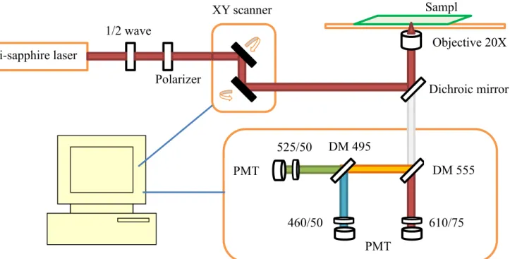
3.1 Laser and microscope
The excitation source used in our multiphoton microscope is generated by the tunable
titanium-sapphire laser (Tsunami, Spectra-Physics) pumped by a diode-pumped laser (Millennia X, Spectra-physics). The titanium-sapphire laser is tuned to satisfy the two-photon excitation condition.
The wavelength of the laser is 780 nm and the laser is pulsed with approximate 100 fs pulse width and at the repetition rate of 80 Mhz. The advantage of using the wavelength near-infrared is the reduction of the scattering and absorption when light passing through the biological sample.
To adjust the power of the laser, a half wave plate followed by a linear polarizer is set on the light path. By rotating the half wave with touching the linear polarizer, we can adjust the power and keep the polarization. Scanning of the laser beam on the focal plane is handled by a set of
galvanometer-driven mirrors (Model 6210, Cambridge Technology, Cambridge, MA). One mirror rotates along the horizontal axis and the other rotates along the vertical axis. By the rotation of the mirrors, plane scanning is achieved. We also called the scanning system x-y scanner. The x-y scanner is controlled by the computer and by each scan we get a frame of plane image at specific depth. There are several scanning modes which we could alter for different sizes of scanning plane, resolution of a frame image (pixels/frame), scanning speed (pixels/second). After the x-y scanner, the beam is directed into a microscope. The objective (20X, S Flour, NA 0.75, Nikon) is used to focus the laser beam on the sample. The sample is placed on a x-y-z movable stage which is controlled and located by the computer. By moving the stage in the z-direction with the sample fixed on, we can get 3-dimesional information of the sample. The emitted fluorescence signal excited by the laser will collected by the same objective. The collected signal then passes through the dichroic mirror and enters the detection box called PMT box by us. In the PMT box, the signal
will be separated into three detection channels by a set of dichroic mirrors (555DCLP, 495DCXR, Chroma Technology, Rockingham, VT) and additional band-pass filters (HQ460/50,
HQ525/50,HQ610/75, Chroma Technology). The signals are finally registered by the
photomultiplier tubes (R7400P, Hamamatsu, Japan) in the single photon counting mode. The output from the PMT are processed by a discriminator and transferred to the computer.
Two-photon microscope
Polarizer
Sampl XY scanner
460/50 610/75
Dichroic mirror 1/2 wave
Ti-sapphire laser
DM 555 525/50 DM 495
PMT box PMT PMT
Objective 20X
Figure 3.1.1 Laser and microscope system
3.2 Stain
DAPI, (4',6-diamidino-2-phenylindole) was first synthesized in Otto Dann’s laboratory at Erlangen and the fluorescence enhance when attached to DNA was found by Williamson and Fennell in 1975.
DAPI is a blue-fluorescence stain which preferentially binds to the double-stranded DNA which is especially rich in adenine-thymine sequences. The complex formed by the binding of DAPI and DNA produces approximately 20-fold fluorescent enhancement. The maximum excitation wave length is 358nm and the maximum emission wave length is 461nm for DAPI bound to DNA. DAPI also binds RNA. However the fluorescence is much weaker compared to the fluorescence of
DAPI-DNA complex. The wavelength of the DAPI-RNA complex also shifts from ~460nm yielded by DAPI-DNA complex to ~500nm.
When using DAPI for the quantitative DNA measurement, there are some points which is worth noting. DAPI is a base specific stain which has the high affinity A-T rich DNA sequence. Hence, the fluorescence intensity depends not only on the amount of DNA but also the content of the A-T base of the DNA. Moreover, the degree of chromatin condensation which depends on the method of cell preparation also affects the amount of the DAPI bound in the cell. For example, washing cells with 0.1N hydrochloric acid to remove histone proteins approximately doubles the amount of DAPI bound to DNA[12].
DAPI can be used on the live or fixed cells. However the efficiency of DAPI passing through the live cells is less than the fixed cells. The effectiveness of the stain is lower. DAPI is also popular in multicolor fluorescent techniques. Due to the blue fluorescence, DAPI has a vivid contrast to green, yellow, or red fluorescent probes of other structures.
Figure 3.2.1 chemical formula of DAPI
Figure 3.2.2 DAPI bind to DNA
Figure 3.2.3 Excitation and emission spectrum of DAPI
3.3 cell line CL1[14]
CL1 was the human lung cancer cell line established from a 64-yr-old man with a poorly
differentiated adenocarcinoma. By the xenograft experiment which demonstrates tumor formation, it shows that CL1 cell line still keep the characteristics of adenocarcinoma even if the cells have been cloned and passed on for more than 60 generations. To better understand the mechanisms underlying invasiveness and metastasis, five sublines (CL1-1, CL1-2, CL1-3, CL1-4 and CL1-5) with progressive invasiveness and metastatic capabilities were obtained through the in vitro selection process. The selection process is a loop that from CL1-0, CL1-1 is selected and CL1-2 is selected from CL1-1, and so on. The Transwell plates which have the polycarbonate membranes containing 8μm pores and coated with Matrigel are used for the selection of invasiveness. Cells were resuspended in RPMI, the cell culture medium, and seeded into the wells. After the incubation for 72 hours at 37oC, remove the well and harvest the cells that migrated through the membranes and attached to the lower-chamber compartments. One round of the invasiveness selection is finished. We can culture the cells and expand them for next round selection.
By the similar way, the experiment of the invasion activity can be conducted. The result showed that the invasive potential of CL1-5 increased by 4- to 6-fold compared to CL1-0.
membrane
Cells CL1-0
Cells invade through the membrane 72 h
3.4 Preparation for the sample Cell culture
The cells we used in our experiment are CL1-0 and CL1-5 cell lines established by Chu et al. and provided by professor Huei-Wen Chen (National Taiwan University College of Medicine Graduate institute of Toxicology).
The cell lines are cultured in RPMI 1640 media (Invitrogen, Carlsbad, CA, USA) supplemented with 10% fetal bovine serum (GIBCO, Carlsbad, CA, USA) and 1% antibiotics (GIBCO), and maintained in an incubator with humidified atmosphere of 5% CO2 and 95% air at 37oC. Every two days, to avoid the cell density becoming too high, we will split the cells in one cell culture flask into three new flasks and renew the cell culture medium.
Staining
The samples were stained by DAPI and CellTrackerTM Orange CMTMR Dye (Thermo Fisher Scientific). DAPI has blue fluorescence and CellTracker is orange. Two different fluorescent signals can be separated by the PMT box introduced in the section 4.1(DAPI excitation:358nm
emission:461nm, CellTracker excitation:541nm emission:565nm). In this thesis, only the DAPI signals will be considered for analysis. The CellTracker signal is adapted by another thesis.
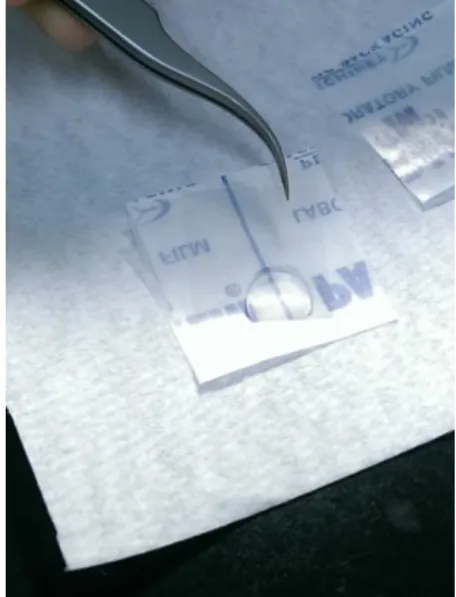
Before staining, the cells need to be seeded on the cover slip which is coated by the 3mg/mL type I collagen diluted 20 times with Phosphate-buffered saline (PBS). The seeded cell concentration is 2X10⁵ cells/mL calculated with the counting chamber. The live cells are first stained with CellTracker of which the concentration is 0.5μM in serum-free medium in the incubator for 30 minutes. Then the cells are fixed with the 3.7% formalin solution before the staining of 0.5mg/L DAPI diluted by PBS from stock solution. To stain the DAPI, we drop 100μL DAPI on the
Parafilm and place the cover slip on the drop with the side seeded the cells. After staining, we add 10μL PBS solution between cover slip and slide, and mount them with nail polish coated around the cover slip.
3.5 Setting of microscope and operation procedure
The images of the samples are scanned by the system described in 3.1. The setting of the
microscope is in scan mode large FOV(340μm x 340μm scanning plane), scanning speed 20kHz, resolution of the image (512 x 512), and scanning along z-direction for 30 layers that the distance between each layer is 1μm. The highest intensity appears at the middle layer. After the z-scan for the area is finished, we can move the stage in x-y plane for the scan of other areas of the samples.
The laser intensity can be adjusted by rotate the half wave plate and its value is measured by a portable power meter placed after the polarizer. The excitation intensity for the z-scan is about 300mW.
Figure 3.4.1 the method to stain DAPI
Figure 3.4.2 complete sample
Chapter 4 Result and discussion
4.1 Image processing
The signals acquired by the microscope are separated to different channel by the wave bands, 610/75(nm), 525/50(nm), 460/50(nm). We take the images of DAPI in channel 525/50 for analysis since it shows the highest intensity in our system (signal of DAPI in 525/50 is a little stronger than in 460/50, and there is no DAPI signal in 610/75). The images are processed with a public domain program, ImageJ. To quantify DNA content of cells, we need to segment nucleus from the image and acquired the integrated intensity of each nucleus (the sum of the intensity value of each pixel in the nucleus). The following is the procedure to process the image and is all done with ImageJ.
With the 30 stacks of images, first sum their intensity into one image (image/stacks/z project/sum slices). To segment the nucleus, the image needs to be adjusted the threshold and transformed to
binary form. There are several methods which have different outcomes and may affect the result of the nucleus segmentation. The method used in this thesis is in image/adjust/auto threshold/method Huang. After autothreshold, use the function, watershed (process/binary/watershed), which can
separate two connected nuclei and analyze particles (analyze/analyze particles) for nucleus
segmentation. In the function, analyze particles, one can set the limit of minimum size (pixel^2) of the nucleus and exclude all small noise (set the minimum size limit, 150). The selection information is then stored in the ROI manger. To acquire the data, use measure in ROI manager on the original image.
Figure 4.1.1 Image processing and data acquisition
4.2 z-stack summation image
Considering the nucleus in the cell attached on the cover slip is not a completely flat object, the z-scan is used to quantify the total DNA content of the nucleus. The Figure (4.2.1) shows the integrated intensity of each cell from two image that one is single layer which has the highest intensity in the z-stacks and the other is the image of which the intensity is the summation of the z-stacks.
The spatial distributions along the z-axis of the nuclei on the cover slip are similar that most of them have the highest intensity in the same layer and the effect of z-summation simply is the linear intensity enhancement. The advantage of the enhancement is that the cell segmentation becomes more precise and it reflects the total DNA content. However it takes time which is proportional to the number of the scanning stacks. If the analysis only needs DNA content, the scan of z-stacks is unnecessary.
y = 1.8391x + 751.78 R² = 0.9799
0 20000 40000 60000 80000 100000 120000 140000
0 10000 20000 30000 40000 50000 60000 70000 80000
z-stacks summation
single layer
integrated intensity of each nucleus
Figure 4.2.1 integrated intensity of cells in z-stack summation image – in highest intensity single layer image
There is also a problem that should be noticed in this experiment. The enhancement ratio which defined as the slope in the Figure (4.2.1) is not a stable value. With the condition that the same sample and the successive scans, the enhancement ratios of the different z-stacks summation vary approximately from 2 to 9. The difference may be caused by the different overlapping volume of the two-photon excitation volume from different layers which is related to the laser intensity.
4.3 Comparison of CL1-0 and CL1-5
According to some measurements of DNA content by flow cytometry, the DNA content distribution of a group of the same species cells can be divide into three divisions which represent the different phases of the cycle, G1 phase, S phase and G2/M phase[13]. G1 phase is from the end of the mitosis until the DNA beginning to synthesis for cell duplication. When DNA is synthesizing until double content, the cell cycle is in the S phases. In G2/M phase, DNA in the cells remains double in G2 phase then entering the mitosis phase. Generally, most of the cells are in G1 phase that shows the largest peak in the distribution histogram. G2/M phase also has a smaller peak. However the nucleus in the late mitosis stage may be recognized as two objectives by the cell segmentation algorithm, some of the G2/M population will be classified into G1 phase.
As mention in the discussion 4.2 that laser intensity may not be stable, the fluorescence signal should be normalized before combining all the data together. To normalize, all integrated intensities of the cell in same image are divided by the median integrated intensity which has high probability in G1 phase. Then the peak of the normalized distribution will appear at the integrated intensity which has value equal to 1. There are 1324 CL1-0 nuclei and 984 CL1-5 nuclei for the analysis. The integrated intensity distribution histogram of CL1-0 and CL1-5 are shown below.
0 100 200 300
0.2 0.6 1 1.4 1.8 2.2 2.6 3 3.4 3.8
cell number
nucleus integrated density (normalized with the median intensity)
CL1-5
0 100 200 300
0.2 0.6 1 1.4 1.8 2.2 2.6 3 3.4 3.8
cell number
nucleus integrated density (normalized with median intensity)
CL1-0
The two distributions seem similar that both of them have the G1 peaks and without the G2/M peak.
Trying to differentiate two cell lines by the integrated intensity data, the average value and the standard deviation are calculated. The mean and standard deviation of CL1-0 and CL1-5 are (1.085, 0.514) and (1.163, 0.715). Though the difference looks small, that the both larger values of CL1-5 seems to suggest that CL1-5 has higher DNA content abnormality. Because of DNA
synthesis, the signals of normal and abnormal DNA content are merged in the distribution
histogram. To avoid the problem, another attempt to find the difference of cell lines is to count the nuclei of which the integrated intensity is larger than 2.6. There are 1.1% nuclei of CL1-0 and 4.5%
nuclei of CL1-5 satisfying the condition that also suggest the higher DNA abnormality of CL1-5.
Use the same method on the analysis of nuclei area. We can see that CL1-0 nuclei are larger than the CL1-5 nuclei and the dispersion of the CL1-0 area is also larger. From the Figure 4.3.3, it shows that the integrated intensity increase with the area. However the distribution histograms of
integrated intensity seem to be different from the distributions of the area. We also wonder how the distribution of average intensity is.
Figure 4.3.1 Integrated intensity distribution histogram of CL1-0 and CL1-5
0 1 2 3 4 5 6
0 200 400 600 800 1000
integrated intensity
area (μm^2)
CL1-5
0 1 2 3 4 5 6
0 200 400 600 800 1000
integrated intensity
area (μm^2)
CL1-0
0 50 100 150
cell number
area (μm^2)
CL1-0
0 50 100 150
cell number
area (μm^2)
CL1-5
To get the average intensity, integrated intensity of each nucleus is divided by its area. The origin average intensity is also normalized by multiplying the same value which makes the mean of average intensity equal to the mean of integrated intensity. The distribution of the average intensity shows that most of the nuclei of CL1-0 have the value 1 average intensity. But the nuclei of CL1-5 have the similar counts from average intensity 1 to 1.4 that may imply the disperse DNA density in the CL1-5 nuclei.
Figure 4.3.2 area distribution histogram of CL1-0 and CL1-5
Figure 4.3.3 integrated intensity – area diagram of CL1-0 and CL1-5
0 100 200 300 400 500
0.2 0.6 1 1.4 1.8 2.2 2.6 3 3.4 3.8
cell number
nucleus average density (integrated intensity/area)
CL1-0
0 100 200 300
0.2 0.6 1 1.4 1.8 2.2 2.6 3 3.4 3.8
cell number
nucleus average intensity (integrated intensity/area)
CL1-5
Table 4.4.1 Statistical value of some quantities of CL1-0 and CL1-5 Conclusion
Though the difference of the two cell lines can be recognize from the histograms, it is more convenient to have a value as the index of two cell lines furthermore the invasive ability. As the table showed below, the percentage difference between the standard deviation of the integrated density is the largest. And it may have the potential to measure the DNA content abnormality and the invasive ability of cells.
CL1-0 CL1-5
Average Standard deviation
Coefficient of variance
Average Standard deviation
Coefficient of variance Integrated
intensity 1.085 0.514 0.474 1.163 0.715 0.615
Area
(μm^2) 282.2 125.3 0.444 258.6 112.3 0.434
Average intensity
1.085 0.408 0.376 1.163 0.380 0.327
Figure 4.3.4 Nucleus average density distribution histogram of CL1-0 and CL1-5
References
[1] 國家衛生福利部, “民國 103 年主要死因分析,” (2016)
[2] Siegel, R., et al. (2013). "Cancer statistics, 2013." CA: A Cancer Journal for Clinicians 63(1):
11-30.
[3] American Cancer Society
[4] Team, T. N. L. S. T. R. (2011). "Reduced Lung-Cancer Mortality with Low-Dose Computed Tomographic Screening." New England Journal of Medicine 365(5): 395-409.
[5] Dyszkiewicz, W., et al. (2000). "Prognostic significance of DNA ploidy in squamous cell lung carcinoma: is it really worth it?" The Annals of Thoracic Surgery 70(5): 1629-1633.
[6] Volm, M., et al. (1985). "DNA distribution in non-small-cell lung carcinomas and its relationship to clinical behavior." Cytometry 6(4): 348-356.
[7] Bunn PA, Krasnow St, Makuch RW, Schlam ML, Schechter GP: Flow cytometry analysis of DNA content of bone marrow cells in patients with plasma cell myeloma: Clinical implications.
Blood 59528-535, 1982.
[8] Choma, D., et al. (2001). "Aneuploidy and prognosis of non-small-cell lung cancer: a meta-analysis of published data." Br J Cancer 85(1): 14-22.
[9] Boyd, R. W., Nonlinear optics, 3rd ed. (Academic, London, 2008)
[10] DeVoe, R. J., et al. (2003). Voxel shapes in two-photon microfabrication.
[11] Born, M & Wolf, E., Principles of optics : electromagnetic theory of propagation, interference and diffraction of light, 7th(expanded) ed. (Cambridge University Press, Cambridge, UK; New York;, 1999)
[12] Kapuscinski, J. (1995). "DAPI: a DNA-specific fluorescent probe." Biotech Histochem 70(5):
220-233.
[13] Roukos, V., et al. "Cell cycle staging of individual cells by fluorescence microscopy."
(1750-2799 (Electronic)).
[14] Chu, Y.-W., et al. (1997). "Selection of Invasive and Metastatic Subpopulations from a Human Lung Adenocarcinoma Cell Line." American Journal of Respiratory Cell and Molecular Biology 17(3): 353-360.