A Parallelized Learning Algorithm for Monotonicity Constrained Support Vector Machines

(1)

A Parallelized Learning Algorithm for

Monotonicity Constrained Support

Vector Machines

Authors：H. C. Chuang, C. C. Chen, C. Chou, Y. C. Cheng, S. T. Li Presenter：Hui-Chi ,Chuang

(2)

2

Agenda

Introduction

Literature Review

Research Methodology

Experimental Results and Analysis

Conclusions and Suggestions

(3)

3

Agenda

Introduction

Literature Review

Research Methodology

Experimental Results and Analysis

Conclusions and Suggestions

(4)

4

Computers

Server

Research Background and Motivation(1/3)

Mobile phones

Surveillance device smart appliances

(5)

Research Background and Motivation(2/3)

 Support Vector Machines (SVMs) are widely used data

mining techniques owing to their excellent abilities in solving both classification and regression problems.  Data mining techniques enable us to discover hidden

patterns and extract valuable knowledge from databases.  Knowledge-driven：Take a priori domain knowledge into

account.

 Some monotonic relationships exist between attributes and the output values.

(6)

Research Background and Motivation(3/3)

SVM with Monotonicity Constraints(MCSVM)

• Advantage:

1.More accuracy and meaningful

2.Reduce the interference of noise data

• Disadvantage:

1.Change the structure of quadratic programming problem

2. High computing time O (

𝑁𝑁

2

𝑀𝑀)

(7)

Research Objectives

MCSVM

SVM Monotonicity Constrain

Parallel Strategy

(8)

8

Agenda

Introduction

Literature Review

Research Methodology

Experimental Results and Analysis

Conclusions and Suggestions

(9)

Support Vector Machine(1/2)

 Vapnik (1995) proposed support vector machine, SVM)  It is a kind of data mining methods that have been

successively proposed and widely discussed.

 It is sensitive to outliers or noises in the training sample due to overfitting. (Guyon, Matic, Vapnik, 1996)

 SVM is designed to minimize the structural risk by minimizing an upper bound of the generalization error rather than the training error.

(10)

Support Vector Machine(2/2)

Optimal Hyperplane O O O O O x x x x _x x O Support Vectors Support Vectors min 1 2 𝒘𝒘 2 + 𝐶𝐶 �_𝑖𝑖=1 𝑁𝑁 𝜀𝜀_𝑖𝑖 , 𝑠𝑠𝑠𝑠𝑠𝑠𝑠𝑠𝑠𝑠𝑠𝑠𝑠𝑠 𝑠𝑠𝑡𝑡 𝑦𝑦_𝑖𝑖 𝒘𝒘𝑻𝑻𝝋𝝋 𝒙𝒙_𝒊𝒊 + 𝑠𝑠 ≥ 1 − 𝜀𝜀_𝑖𝑖, 𝑖𝑖 = 1, … , 𝑁𝑁, 𝜀𝜀_𝑖𝑖 ≥ 0, 𝑖𝑖 = 1, … , 𝑁𝑁

𝒘𝒘: normal vector to the hyperplane,

𝜺𝜺_𝒊𝒊: distance between the outlier 𝑖𝑖 and hyperpla 𝑪𝑪: constant, regarded as a regularization param 𝝋𝝋 𝒙𝒙 : kernel function

(11)

Monotonicity Constraints

 There are two different approaches for dealing with problems that have prior knowledge of monotonic properties.

 One is to apply a relabeling technique to those data missing monotonicity

 The other is to add the monotonicity constraints directly to the optimization modeling settings

(12)

Monotonicity Constrained SVMs (1/2)

 Monotonicity is a relationship in which increasing the value of the variables always increases or decreases the likelihood category membership.

 Define the monotonicity relationship.

 Given a dataset with denoted as the feature space, and a partial ordering defined over this input space .

 A linear ordering is defined over the space Y of class values .

(

)

{

_i , y_i |i 1, 2,...,N

}

ℑ = x =

≤

n R

≤

i y

(13)

Monotonicity Constrained SVMs (2/2)

 Then the classifier is monotone if the following statement holds:

 The monotonicity constraints can be expressed as the following inequality: , for all

( )

, , i ≤ j ⇒ f i ≤ f j ∀i j x x x x ( ) ( ) T T i j ϕ ≤ ϕ w x w x x_i ≤ x_j

(14)

14

Parallel Strategy

 The concept of “ Divide and Conquer. “

 Collobert et al. (2002) - Can be easy to implemented in parallel and where each SVM is trained on a small

subset of the whole dataset.

 Kruger et al. (2006) - Mixture of SVM for speech recognition using Hidden Markov Model

(15)

15

Agenda

Introduction

Literature Review

Research Methodology

Experimental Results and Analysis

Conclusions and Suggestions

(16)

16

Construct Monotonicity Constraints(1/2)

Algorithm 1: Monotonicity Constraints – Hierarchy Method

Step 1. Determine the Hierarchy partition 𝑧𝑧_𝑖𝑖 = 𝑠𝑠_𝑖𝑖,0, … , 𝑠𝑠_{𝑖𝑖,𝑣𝑣}, … , 𝑠𝑠_{𝑖𝑖,𝑀𝑀} = 𝑧𝑧_𝑖𝑖 for the range interval 𝑧𝑧_𝑖𝑖, 𝑧𝑧_𝑖𝑖 , for𝑖𝑖 = 1,2, … , 𝑛𝑛.

Step 2. Determine 𝒙𝒙_𝒌𝒌= 𝑥𝑥_𝑘𝑘,1, 𝑥𝑥_𝑘𝑘,2, … , 𝑥𝑥_{𝑘𝑘,𝑛𝑛} and 𝒙𝒙_𝒌𝒌 = 𝑥𝑥_𝑘𝑘,1, 𝑥𝑥_𝑘𝑘,2, … , 𝑥𝑥_{𝑘𝑘,𝑛𝑛} such that

𝑥𝑥𝑘𝑘,𝑖𝑖 = 𝑠𝑠𝑖𝑖,𝑘𝑘−1𝑖𝑖 ∈ 𝑀𝑀𝑖𝑖𝑛𝑛𝑖𝑖 , 𝑥𝑥𝑘𝑘,𝑖𝑖 = 𝑠𝑠𝑖𝑖,𝑘𝑘 𝑖𝑖 ∈ 𝑀𝑀𝑑𝑑𝑖𝑖𝑑𝑑 , 𝑥𝑥𝑘𝑘,𝑖𝑖 = ∀ 𝑠𝑠𝑣𝑣 𝑖𝑖 ∈ 𝑀𝑀𝑛𝑛𝑛𝑛𝑛𝑛𝑛𝑛 ,

𝑥𝑥𝑘𝑘,𝑖𝑖 = 𝑠𝑠𝑖𝑖,𝑘𝑘 𝑖𝑖 ∈ 𝑀𝑀𝑖𝑖𝑛𝑛𝑖𝑖 , 𝑥𝑥𝑘𝑘,𝑖𝑖 = 𝑠𝑠𝑖𝑖,𝑘𝑘−1 𝑖𝑖 ∈ 𝑀𝑀𝑑𝑑𝑖𝑖𝑑𝑑 , 𝑥𝑥𝑘𝑘,𝑖𝑖 = ∀ 𝑠𝑠𝑣𝑣 𝑖𝑖 ∈ 𝑀𝑀𝑛𝑛𝑛𝑛𝑛𝑛𝑛𝑛 ,

for 𝑖𝑖 = 1,2, … , 𝑛𝑛, 𝑘𝑘 = 1,2, … , 𝑀𝑀 and 𝑣𝑣 = 0,1,2, … , 𝑀𝑀. Step 3. Add the monotonicity constraint𝒘𝒘𝑇𝑇𝝋𝝋 𝒙𝒙_𝒌𝒌 ≤ 𝒘𝒘𝑇𝑇𝝋𝝋 𝒙𝒙_𝒌𝒌 . Hierarchy Method (Yang, 2014)

(17)

17

Construct Monotonicity Constraints(2/2)

Level Level 1 Level 2 Level 3

Attribute A1 A2 A3 A1 A2 A3 A1 A2 A3 Max Min v11 v15 v21 v25 r3 v11 v15 v21 v25 r3 v13 v23 v11 v15 v21 v25 r3 v13 v23 v14 v12 v24 v22 𝑥𝑥1= (v15,v21,r3) 𝑥𝑥1= (v11,v25,r3) 𝑥𝑥2= (v15,v23,r3) 𝑥𝑥3= (v13,v21,r3) 𝑥𝑥2= (v13,v25,r3) 𝑥𝑥3= (v11,v23,r3) 𝑥𝑥4= (v15,v24,r3) 𝑥𝑥5= (v14,v23,r3) 𝑥𝑥6= (v13,v22,r3) 𝑥𝑥7= (v12,v21,r3) 𝑥𝑥4= (v14,v25,r3) 𝑥𝑥5= (v13,v24,r3) 𝑥𝑥6= (v12,v23,r3) 𝑥𝑥7= (v11,v22,r3)

𝒘𝒘

𝑇𝑇

𝝋𝝋(𝒙𝒙

_𝒌𝒌

) ≤ 𝒘𝒘

𝑇𝑇

𝝋𝝋(𝒙𝒙

_𝒌𝒌

)

(18)

Adding the monotonicity constraints to SVM, the model become as following:

18

SVM with Monotonicity Constraints(1/3)

min J 𝒘𝒘, 𝛆𝛆 = 1_{2 𝒘𝒘} 2 + 𝐶𝐶 � 𝑖𝑖=1 𝑁𝑁 𝜀𝜀_𝑖𝑖, 𝑠𝑠𝑠𝑠𝑠𝑠𝑠𝑠𝑠𝑠𝑠𝑠𝑠𝑠 𝑠𝑠𝑡𝑡 𝑦𝑦_𝑖𝑖 𝒘𝒘𝑻𝑻𝝋𝝋 𝒙𝒙_𝒊𝒊 + 𝑠𝑠 ≥ 1 − 𝜀𝜀_𝑖𝑖, 𝑖𝑖 = 1, … , 𝑁𝑁, 𝒘𝒘𝑻𝑻𝝋𝝋 𝒙𝒙 ≤ 𝒘𝒘𝑻𝑻𝝋𝝋 𝒙𝒙 , 𝜀𝜀_𝑖𝑖 ≥ 0, 𝑖𝑖 = 1, … , 𝑁𝑁.

(19)

The problem use the Lagrangian multiplier will be turned into following form:

19

SVM with Monotonicity Constraints(2/3)

max_{𝜶𝜶,𝜷𝜷} 𝑄𝑄�(𝜶𝜶, 𝜷𝜷) = � 𝛼𝛼𝑖𝑖 −1_{2 � � 𝛼𝛼}𝑖𝑖𝛼𝛼𝑠𝑠𝑦𝑦𝑖𝑖𝑦𝑦𝑠𝑠𝝋𝝋(𝒙𝒙𝒊𝒊)𝑻𝑻 𝑁𝑁 𝑠𝑠=1 𝑁𝑁 𝑖𝑖=1 𝑁𝑁 𝑖𝑖=1 𝝋𝝋�𝒙𝒙𝒋𝒋� −1_{2 � � 𝛽𝛽}𝑘𝑘𝛽𝛽𝑙𝑙 �𝝋𝝋(𝒙𝒙𝒌𝒌) − 𝝋𝝋�𝒙𝒙𝒌𝒌�� 𝑇𝑇 𝑀𝑀 𝑙𝑙=1 �𝝋𝝋(𝒙𝒙𝒍𝒍) − 𝝋𝝋�𝒙𝒙𝒍𝒍�� 𝑀𝑀 𝑘𝑘=1 −1_{2 � � 𝛼𝛼}𝑖𝑖𝑦𝑦𝑖𝑖𝛽𝛽𝑘𝑘 𝑀𝑀 𝑘𝑘=1 𝑁𝑁 𝑖𝑖=1 �𝝋𝝋(𝒙𝒙𝒌𝒌) − 𝝋𝝋�𝒙𝒙𝒌𝒌�� 𝑇𝑇 𝝋𝝋(𝒙𝒙𝒊𝒊) −1_{2 � � 𝛼𝛼}_𝑖𝑖𝑦𝑦_𝑖𝑖𝛽𝛽_𝑘𝑘 𝑀𝑀 𝑘𝑘=1 𝑁𝑁 𝑖𝑖=1 𝝋𝝋(𝒙𝒙_𝒊𝒊)𝑻𝑻_{�𝝋𝝋(𝒙𝒙} 𝒌𝒌) − 𝝋𝝋�𝒙𝒙𝒌𝒌��, 𝑆𝑆𝑠𝑠𝑠𝑠𝑠𝑠𝑠𝑠𝑠𝑠𝑠𝑠 𝑠𝑠𝑡𝑡 �𝛼𝛼𝑖𝑖𝑦𝑦𝑖𝑖 = 0, 𝑁𝑁 𝑖𝑖=1 0 ≤ 𝛼𝛼𝑖𝑖 ≤ 𝐶𝐶, 𝑖𝑖 = 1, … , 𝑁𝑁, 𝛽𝛽𝑘𝑘 ≥ 0, ∀𝑘𝑘 = 1, … , 𝑀𝑀.

(20)

Rewrite the problem into the matrix form:

20

SVM with Monotonicity Constraints(3/3)

min_{𝜶𝜶,𝜷𝜷} �𝑄𝑄 𝜶𝜶, 𝜷𝜷 = 1 2 𝜶𝜶𝑇𝑇 𝜷𝜷𝑇𝑇 G 𝜶𝜶 𝜷𝜷 − 1𝑇𝑇𝜶𝜶, 𝑆𝑆𝑠𝑠𝑠𝑠𝑠𝑠𝑠𝑠𝑠𝑠𝑠𝑠 𝑠𝑠𝑡𝑡 �_𝑖𝑖=1 𝑁𝑁 𝛼𝛼_𝑖𝑖𝑦𝑦_𝑖𝑖 = 0, 0 ≤ 𝛼𝛼_𝑖𝑖 ≤ 𝐶𝐶, 𝑖𝑖 = 1, … , 𝑁𝑁, 𝛽𝛽𝑘𝑘 ≥ 0, ∀𝑘𝑘 = 1, … , 𝑀𝑀. G = G11 G12 G21 G22 G_{𝑖𝑖,𝑗𝑗}11 = 𝑦𝑦_𝑖𝑖𝑦𝑦_𝑗𝑗𝝋𝝋 𝒙𝒙_𝒊𝒊 𝑇𝑇𝝋𝝋 𝒙𝒙_𝒋𝒋 , G_{𝑖𝑖,𝑘𝑘}12 = 𝑦𝑦_𝑖𝑖 𝝋𝝋 𝒙𝒙_𝒌𝒌 − 𝝋𝝋 𝒙𝒙_𝒌𝒌 𝑇𝑇 𝝋𝝋 𝒙𝒙_𝒊𝒊 , G21 = G12 𝑇𝑇, G_{𝑘𝑘,𝑙𝑙}22 = 𝝋𝝋 𝒙𝒙_𝒌𝒌 − 𝝋𝝋 𝒙𝒙_𝒌𝒌 𝑇𝑇 𝝋𝝋 𝒙𝒙_𝒍𝒍 − 𝝋𝝋 𝒙𝒙_𝒍𝒍 for 𝑖𝑖, 𝑠𝑠 = 1, … , 𝑁𝑁, 𝑘𝑘, 𝑙𝑙 = 1, … , 𝑀𝑀.

(21)

 The problem output the following optimal solution:

 minimize the cost function

 Mixture function 21

Parallel Strategy-Mixture

𝑓𝑓 𝑥𝑥 = [ℎ � 𝑗𝑗=1 𝑃𝑃 𝜔𝜔_𝑗𝑗(𝑥𝑥)𝑆𝑆_𝑗𝑗(𝑥𝑥)] 𝑆𝑆_𝑖𝑖(𝑥𝑥) = � 𝑖𝑖=1 𝑁𝑁 𝛼𝛼_𝑖𝑖𝑦𝑦_𝑖𝑖𝐾𝐾 𝑥𝑥_𝑖𝑖, 𝒙𝒙 + � 𝑘𝑘=1 𝑀𝑀 𝛽𝛽_𝑘𝑘 𝐾𝐾 𝑥𝑥_𝑘𝑘, 𝒙𝒙 − 𝐾𝐾 𝑥𝑥_𝑘𝑘, 𝒙𝒙 + 𝑠𝑠 𝜔𝜔 = � 𝑖𝑖=1 𝑁𝑁 𝑓𝑓 𝑥𝑥_𝑖𝑖 − 𝑦𝑦_𝑖𝑖 .

(22)

22

Agenda

Introduction

Literature Review

Research Methodology

Experimental Results and Analysis

Conclusions and Suggestions

(23)

23

Experimental Design(1/3)

1. Hardware: Intel Core i7-4770 CPU 3.2 GHz with 16 GB RAM

Software: MATLAB R2015a

2. Kernel function: RBF function

3. Grid search:

C = {0.01 0.05 0.1 0.5 1 5 10 50 100 500 1000},

σ = {0.5 5 10 15 25 50 100 250 500}.

(24)

24

Experimental Design(2/3)

Training Dataset 67% Testing Dataset 33% Dataset RMC-SVM Mixture RMC-SVM Repeat 30 times

(25)

25

Experimental Design(3/3)

Experiment Parts _Constraints } 𝑵𝑵𝒖𝒖𝒖𝒖𝒖𝒖𝒖𝒖𝒖𝒖 𝒐𝒐𝒐𝒐 𝒑𝒑𝒑𝒑𝒖𝒖𝒑𝒑𝒑𝒑 = {𝟐𝟐, 𝟒𝟒, 𝟔𝟔 𝑵𝑵𝒖𝒖𝒖𝒖𝒖𝒖𝒖𝒖𝒖𝒖 𝒐𝒐𝒐𝒐 𝒄𝒄𝒐𝒐𝒄𝒄𝒑𝒑𝒑𝒑𝒖𝒖𝒑𝒑𝒊𝒊𝒄𝒄𝒑𝒑𝒑𝒑 = 𝟔𝟔𝟔𝟔, 𝟏𝟏𝟐𝟐𝟏𝟏

(26)

26

Dataset Collection

Dataset : WDBC

Attribute Type Monotonicity Relationships

Clump thickness Numerical Increasing with Class

Uniformity of cell size Numerical Increasing with Class

Uniformity of cell shape Numerical Increasing with Class

Marginal adhesion Numerical Increasing with Class

Single epithelial cell size Numerical Increasing with Class

Bare nuclei Numerical Increasing with Class

Bland chromatin Numerical Increasing with Class

Normal nucleoli Numerical Increasing with Class

Mitoses Numerical Increasing with Class

Class Class value=4 (malignant): 239 (34.99%)

Class value=2 (benign): 444 (65.01%)

• UCI

• Size : 683 × 9

Table 1. WDBC dataset characteristics and monotonic relationship (http://kdd.ics.uci.edu/)

(27)

27

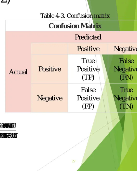
Performance Measures(1/2)

• 𝐴𝐴𝑠𝑠𝑠𝑠𝑠𝑠𝐴𝐴𝐴𝐴𝑠𝑠𝑦𝑦 =

𝑇𝑇𝑃𝑃+𝑇𝑇𝑁𝑁 𝑇𝑇𝑃𝑃+𝐹𝐹𝑃𝑃+𝑇𝑇𝑁𝑁+𝐹𝐹𝑁𝑁

• 𝑅𝑅𝑠𝑠𝑠𝑠𝐴𝐴𝑙𝑙𝑙𝑙 =

𝑇𝑇𝑃𝑃 𝑇𝑇𝑃𝑃+𝐹𝐹𝑁𝑁

• 𝑃𝑃𝐴𝐴𝑠𝑠𝑠𝑠𝑖𝑖𝑠𝑠𝑖𝑖𝑡𝑡𝑛𝑛 =

𝑇𝑇𝑃𝑃 𝑇𝑇𝑃𝑃+𝐹𝐹𝑃𝑃

• 𝐹𝐹 − 𝑚𝑚𝑠𝑠𝐴𝐴𝑠𝑠𝑠𝑠𝐴𝐴𝑠𝑠 = 2 �

𝑃𝑃𝑑𝑑𝑛𝑛𝑖𝑖𝑖𝑖𝑃𝑃𝑖𝑖𝑛𝑛𝑛𝑛�𝑅𝑅𝑛𝑛𝑖𝑖𝑅𝑅𝑙𝑙𝑙𝑙 𝑃𝑃𝑑𝑑𝑛𝑛𝑖𝑖𝑖𝑖𝑃𝑃𝑖𝑖𝑛𝑛𝑛𝑛+𝑅𝑅𝑛𝑛𝑖𝑖𝑅𝑅𝑙𝑙𝑙𝑙 Confusion Matrix Actual Predicted Positive Negative Positive True Positive (TP) False Negative (FN) Negative False Positive (FP) True Negative (TN) Table 4-3. Confusion matrix

(28)

28

Performance Measures(2/2)

• Frequency Monotonicity Rate 𝐹𝐹𝑀𝑀𝑅𝑅 = 𝐹𝐹𝑀𝑀_𝑃𝑃

• where P is the number of observed pairs

• FM is the number of pairs that do not violate the monotonicity.

(29)

29

(30)

30

Agenda

Introduction

Literature Review

Research Methodology

Experimental Results and Analysis

Conclusions and Suggestions

(31)

31

Contributions(1/2)

 RMC-SVM vs The parallelized RMC-SVM

• The training time of the parallel strategy RMC-SVM is less than RMC-SVM when both have the similarly classified results.

 The parallelized RMC-SVM with different part to divide dataset

• The parallel strategy RMC-SVM decreases with the increase of the number of parts.

(32)

32

Contributions(2/2)

 Managerial Implications • The monotonicity constraints • The parallel strategy

 Recommendations of Future Works

• Try different algorithms to solve quadratic problem more efficiently. • Extend the classification problem to multiclass cases.

• Attempt more different number parts to divide whole training dataset. • Improve the method of constructing monotonicity constraints.

(33)

33