Automatic Multi-object Segmentation by Two-phase Snake Processing
CHENG-HUNGCHUANG1,*ANDWEN-NUNGLIE2
1Department of Computer Science and Information Engineering, Asia University, Taiean
2Department of Electrical Engineering, National Chung Cheng University, Taiwan
ABSTRACT
This paper presents a two-phase automatic snake algorithm for the segmentation of multiple objects from noisy or cluttered backgrounds. Traditional snake algorithms are often limited in their ability to process multiple objects and are required to have manually-drawn initial contours and fixed weighting parameters. Our algorithm features two phases: (1) the active-points phase and (2) the active-contours phase. In the first phase, grid points evenly distributed in the image are attracted and moved to form clusters near object boundaries. These clustered active points are then analyzed to obtain convex polygons as initial snake contours in the second phase, where a no-search movement scheme with space-varying weighting parameters is employed. Both the kinetics of active points and deformation of active contours accept our proposed adaptive gradient vector flow (AGVF) field as the contracting forces. Experiments show the stability of the AGVF field and good performance of our snake algorithm in segmenting multiple objects from noisy or cluttered backgrounds.
Key words: image segmentation, active contours model, deformable models, snake model, boundary detection, gradient vector flow.
1. INTRODUCTION
Segmentation has been an important technique for image analysis and understanding for quite a long time. Basically, segmentation can be categorized into two types of algorithms: edge-based and region-based. Edge-based segmentation puts emphasis on detecting significant gray-level changes near object boundaries, while region-based segmentation lies great stress on searching areas of uniform features like gray-value, texture, etc. In this research, we will highlight the edge-based segmentation algorithm and focus on active contour models that have been applied to object boundary detection in the past decades.
The active contours model (also called snakes) was first proposed by Kass, Witkin, and Terzopoulos (1988) for object boundary detection. They applied an energy minimizing function, a weighted combination of internal and external energy, to a deformable contour so as to approach the true object boundaries. The internal energy controls intrinsic continuity force of the contour itself, while the external energy governs the attraction force, such as image gradients, that directs the contour movement. By minimizing the energy function, each snake contour point iteratively searches its new position to approach object boundaries. The model proposed in Kass et al. (1988) performs a global search to optimize the energy function. Later, a number of strategies were proposed to reduce the
* Corresponding author. E-mail: [email protected]
computational complexity of snakes (Williams & Shah, 1992; Lam & Yan, 1994a, 1994b;Mirhosseini& Yan,1997).Thesemethodsaremostly based on a‘greedy’
strategy which searches local 8- or 4-neighbors, instead of the global optimization, to speed up the convergence of snakes. In Wong Yuen, & Tong (1998a), a terminating criterion based on contour length was proposed to enhance the stability and reliability of convergence.
In most technical literature, snake models were developed in terms of internal and external energy items plus combining some constraints for more effectiveness and accuracy. For example, Pardo, Cabello, and Heras (1997) proposed adding an exponential item to the internal energy term to control the movement flexibility of snake points in model-based segmentation of CT scan images. Their algorithm also modified the external energy term by adding gradient, intensity, and edge items to avoid false convergence into local minima. In Lam and Yuen (1998), internal energy was modified to minimize changes in length and curvature between temporal active contours for moving/rotating object tracking. In Kang (1999), the algorithm constrains the internal energy by enforcing the successive snake points to have similarity in local motion, which avoids disordered snake movements. In Pardo and Cabello (2000), a priori knowledge of edge segments was incorporated into the external force, making the snake less sensitive to initial conditions. In Davison, Eviatar, and Somorjai (2000), the authors added additional energy items to the snake model, e.g., the area energy that causes the snake to either expand or contract as a whole and the symmetry energy that prevents unphysical departures of boundaries from symmetry.
One of the drawbacks in traditional snake models is heavy sensitivity to initial contour conditions. In other words, the initial contour must be manually set to be close to the object. Another problem is that snakes have difficulty approaching the concave parts of the object boundaries. In Yuen, Wong, and Tong (1996) and Wong, Yuen, and Tong (1998b), an iterative split-and-merge procedure was proposed to solve this problem. In the split procedure, a snake is divided into a number of segments by control points defined by large gradient changes. Then those segments, classified as not being near object boundaries (according to the external energy information), are moved by the normal forces to approach the concave regions of the object. In the merge procedure, all segments are merged together to recover the closed contour. Ji and Yan (2002a, 2002b) added a gradient potential energy term to the snake function, which forms an additional force to attract contour in areas short of boundary features. Nevertheless, if the initial snake is far from true object boundaries or the image is not abundant with edge or gradient information, the algorithms proposed in Yuen et al. (1996), Wong et al.
(1998), and Ji and Yan (2002a, 2002b) will not approximate true object boundaries accurately. To solve these problems, Xu and Prince (1998) proposed a gradient vector flow (GVF) field as an external force in the snake model. The GVF field is obtained by diffusing large gradients from near object boundaries to other areas. In such a way, even the initial snake is far from true object boundaries, it can also be attracted by the GVF field. The efficiency of gradient diffusion depends on a
paper, we propose an adaptive gradient vector flow (AGVF) field algorithm that can be automatically fine-tuned according to image contents. Our algorithm is also proven to be robust in some areas of noisy images from the experiments.
All snake processings mentioned above require initial contours and manually-adjusted weighting parameters between the internal and external energy terms. Often they cannot process multiple or annular objects. Yuen, Feng, and Zhou (1999) proposed an automatic initialization algorithm for contour detection. Their algorithm radiates a series of straight lines from the image center of gravity. Then the point with the largest gradient on each radial line is selected as the feature point.
For multi-object detection, these feature points and the center of gravity constitute the initial contours. However, their initialization algorithm can only detect multiple objects spreading around the center of gravity and will fail when applied to annularly shaped objects or multiple objects located along one radial line. Matsuda et al. (2000) proposed an active net algorithm to detect target regions. The active net is a rectangular network, in which the lattice points are attracted subject to consistency in color attribute. As the authors mentioned, the active net has difficulty dealing with multiple targets in an image. In Velasco and Marroquin (2003), the authors generated initial particles (seeds) in areas with larger gradient magnitude for automatic initialization. This introduces another issue: that of how to select the threshold values of gradient magnitude for varied images.
The level set method (Osher & Fedkiw, 2001; Deng & Tsui, 2002; Precioso &
Barlaud, 2002) has recently been shown to be a robust, accurate, and efficient technique for image segmentation. This algorithm usually starts from a small circle or even a point within the desired contour and tracks the evolving contour movement with a certain velocity function derived from image gradient and geometric properties. One of the drawbacks of level set techniques is that they require considerable thought in order to construct appropriate velocities for advancing the level set function. Although level set methods provide less sensitivity to initial conditions, they are still required to give initial points or circles which are inside or outside the target contours. Furthermore, the computational cost is high (Precioso & Barlaud, 2002) and results are not good for open or broken contours.
In this paper, we propose a new automatic initialization algorithm based on an AGVF field, which is an extension of the previous study (Chuang & Lie, 2001).
The active-contours processing is developed to accurately detect boundaries of multiple or annular objects based on our previous fast snake model (Lie & Chuang, 2001). Unlike the watersnake proposed by Park and Keller (2001) in which snakes must have the aid of watershed transformation to obtain snake zones in advance, our proposed algorithm is a pure snake processing with automatic initialization.
Our method is featured as a fast, accurate, and fully automatic object segmentation technique.
In Section 2, we address some basic snake models as necessary backgrounds.
In Section 3, the proposed fully automatic segmentation algorithm based on the AGVF field is described. In Section 4, simulations and performance analysis are demonstrated. Finally, Section 5 draws some conclusions.
2. SNAKE BACKGROUNDS
The traditional snake model is a conjunction of internal and external energy, by which a contour is animated and deformed towards object boundaries.
Principally, the minimized internal energy maintains smoothness and compactness of the contour shape, but causes degeneration to a single point in the extreme case.
The minimized external energy however adjusts the contour to be consistent with the environmental status where it is located. They can be considered as two forces that guide the snake to move. The model is generally described to be an energy-minimizing function
1
0
) ) ( ( )) (
(v s E v s ds E
Esnake int ext , (1)
where v(s) is the active contour, arc length s[0.0, 1.0], and Eint and Eext are the internal and external energy, respectively. The internal energy is further defined to be
) ) ( ) ( ) ( ) ( 2(
1 2 2
s v s s v s
Eint s ss , (2)
where(s) and(s) are weighting parameters and vs(s) and vss(s) are the 1stand 2nd derivatives of v(s) to represent the continuity and stretch forces of the contour. Eext
is often defined to be the negative of image gradient magnitudes:
)2
, (x y I
Eext , or Eext (G*I x y( , ))2, (3)
where I(x, y) represents the image, is the gradient operator, and Gσis the Gaussian filter with standard deviation . Obviously, object boundaries that often have larger gradient magnitudes will lead to a smaller external energy status. This moves snake contours towards the object boundaries when the external energy is minimized. Overall, the snake model represents a compromise between the internal and external energy statuses via the weighting parameters.
During the energy-minimizing process, the previous greedy algorithms (Williams & Shah, 1992; Lam & Yan, 1994a, 1994b; Mirhosseini & Yan, 1997) adopt a local search scheme instead of global optimization. Each snake point i searches its next position among m-neighbors by comparing the snake energy
, i snake j
E :
, ( ) , ( ) , ( ) ,
i i i i
snake j cont j curv j image j
E i E i E i E , (4)
where j = 1,2,…,m represents the index of a neighborhood (m is the number of neighbor points), ,
i cont j
E and ,
i curv j
E correspond to the continuity and curvature (stretch) forces in the internal energy, ,
i image j
E is the external energy, and α(i), β(i), and γ(i) are weighting parameters which are possibly position-dependent. The computational complexity is thus reduced. However, the snake contours become more sensitive to local noise.
On the other hand, an active contour model based on the GVF field (Xu &
Prince, 1998) is less sensitive to the initial contour conditions. The GVF field is defined to be a field of vectors. Each vector V(x, y) = ( p(x, y), q(x, y)), for any image pixel (x, y), is computed by minimizing the energy function:
2 2
2 2 2 2
(px py qx qy) f V f dxdy
, (5)wheref is the gradient of the edge map f derived from the input image I(x, y), μis a regularization parameter, and the subscripts represent partial derivatives with respect to the x and y axes. After the minimization process, V(x, y) will approximate
f where it is large and be smooth elsewhere, i.e., the gradients are diffused from object boundaries to homogeneous regions. Each GVF vector will point towards the object boundaries even if the currently considered pixel is far from them. The GVF field is then adopted as the external energy term for stronger resistance to noise than the traditional gradients only. Consequently, the snake model based on the GVF field can approach object boundaries even if the initial contour is located far from objects.
3. THE PROPOSED AGVF AND TWO-PHASE SNAKE PROCESSING
Our new multi-object segmentation scheme is composed of two phases: (1) the active-points phase and (2) the active-contours phase. The block diagram of the proposed scheme is shown in Figure 1. It can be considered as a coarse-to-fine segmentation method. In the first phase, approximate positions of the object boundaries are automatically searched to form the initial contours for following snake refinement. This work makes manual setting of initial contours unnecessary and is also suitable to multi-object cases. In the second phase, each contour will be deformed to approach object boundaries progressively. Both phases are based on the AGVF field.
3.1 Adaptive GVF (AGVF) Field
As mentioned in Xu and Prince (1998), the goal of GVF field is to diffuse gradients of edge responses into the whole image so that the external forces towards object boundaries can be effective even for distant pixels. In Eq. (5) the
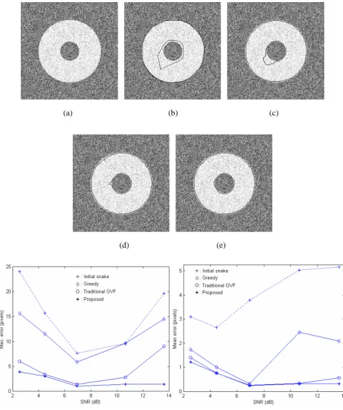
energy εconsists of two terms. The first term is related to the smoothness of the resulting GVF field (smaller value for smoother distribution). The second term computes errors between the GVF field V(x, y) and the original gradient of edgef.
Since the weighting of |V-f |2is squarely proportional to the gradient magnitude
|f |, it will dominate the error where |f | is large (i.e., V(x, y) will be approximate tof ). The parameter μcontrols the trade-off between these two terms. For noisy images, one should increase μto enhance the smoothness of the GVF field, but this will simultaneously cause degraded approximation near object boundaries. Hence, how to give a proper regularization parameter μwill confuse most of the users. In our proposed AGVF field, the weighting parameters are adaptively computed from
f, i.e., they are space-varying. First, the r-order magnitude of the edge gradient,
|f |r, is linearly mapped to the interval [0,1]. That is
| ( , ) | min{| ( , ) | } ( , )
max{| ( , ) | } min{| ( , ) | }
r r
r r
f x y f x y
w x y
f x y f x y
.
(6)
Figure 1. Block diagram of proposed two-phase snake processing scheme.
The power magnitude r is tested in the interval [0.1, 5] with an increment 0.1 and it is found that r = 2.8 has the best performance. Therefore, r is empirically chosen to be 2.8 in subsequent experiments. This step is to normalize the weighting functions in the proposed AGVF field so that they can adapt to images with obscure object boundaries. We denote the weighting functions of the first and the second terms to be κ(x, y) and λ(x, y), respectively. Then Eq. (5) can be rewritten as
2 2 2 2 2
( , )(x y px py qx qy) ( , )x y VAGVF f dxdy
, (7)where
1 ( , ) ( , )
4 w x y
x y , (8)
and
( , )x y w x y( , )
. (9)
The convergence of the AGVF field can be reached when the energy value is (within a threshold) further minimally decreased. Basically, the main goal of this iterative process is to diffuse gradients to form the force field all over the image.
Our AGVF field utilizes the normalized gradients of edge (i.e., w(x, y)) as the weighting parameters between the smoothness and the gradient-approximating terms. Normally, the gradient of edge |f | is small in homogeneous regions and large near object boundaries. Hence, the desired AGVF field will put great emphasis (up to κ= 0.25) on the smoothness term in homogenous regions (where
0
w ) and on the gradient-approximating term elsewhere. These two weighting functions κ(x, y) and λ(x, y) form a linear function λ(x, y) + 4κ(x, y) =1.0 and expect to dominate each other in specific regions. These characteristics of the AGVF field make a higher resistance to noise than the traditional GVF field. After the AGVF field is obtained, it is used for both active-points and active-contours phases. More detailed performance analysis is given in Section 4.2.
3.2 Active-Points Phase
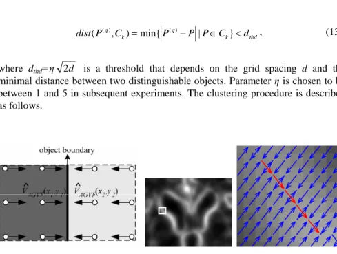
Traditional snake processing for detecting object boundaries demands manually drawing an initial contour. Some others often set the image border as the initial contour for automation. However, this can only be suitable for a single and non-holed object. To cope with the multi-object problem, we propose to explode the initial contour into pixels and distribute them at grid points everywhere in the image, e.g., Figures 8(b), 9(b), and 10(b). Essentially, the grid spacing should be less than the minimum distance that any two neighboring objects can be distinguished. We assume that the grid spacing is d. On processing, these grid pixelsare“independently”moved by adirectionaldriving function,which isbased on the AGVF field. Recognizing this dynamic behavior, they are then meaningfully described asthe“activepoints.”TheroleoftheAGVF field hereisacting asan external force to direct active points towards multi-object boundaries. The internal force is ignored in this phase since no sequential orders exist between these active points.
To be more efficient, the movement of active points is allowed on the grid space only. Hence, we consider only the direction of AGVF vectors and quantize them into 8 directions, i.e., VˆAGVF(x,y)(pˆ(x,y),qˆ(x,y)) , where
d d
y x
pˆ( , ),0, and qˆ(x,y)
d,0,d
. Since VAGVF(x, y) is expected topoint towards object boundaries, direction contradiction may occur for points residing on the opposite sides of boundaries with strong strength and make active points moving back and forth between them. To eliminate this situation and have easier convergence, we remove force contradictions before processing. That is, for grid points (x1, y1) and (x2, y2) that are adjacent and have
) , ˆ (
1 1 y x
VAGVF =VˆAGVF(x2,y2) (as shown in Figure 2(a)), we set both VAGVF(x1, y1) and VAGVF(x2, y2) to (0, 0). Once active points move there, they will stop moving further. Force contradiction may also occur near noisy edges, but not on dim edges.
The driving function of active points is defined to be
, 1( , ) , ( , ) ˆ ( , )
i j i j AGVF
P x y P x y V x y , (10)
where Pi, j(x, y) specifies the coordinates of the i-th unrepeatable active point at the j-th iteration. The active points are initialized at grid pixels. When more than two active points move to an identical position, they will be merged together. This iterative process continues until no change in active-point positions, i.e., the stop criterion of active-points phase is:
, 1 , 0
i j i j
P P , for all i. (11)
Notice that the AGVF vectors may point along the boundaries due to non-uniform gradient magnitudes (i.e., gradient on gradients), as shown in Figures 2(b) and (c).
In this case, active points may cluster around some local minima, rather than the whole boundaries. To overcome this problem, a movement with a large direction change should be also prohibited and stopped if the following criterion is satisfied during the iterative process:
, 1 , 1 2 , , 1
i j i j i j i j
P P P P . (12)
Figure 3 gives an example to demonstrate the behavior of iterations vs.
convergence of active points. It is found that active points converge after 18 iterations to the result in Figure 8(c).
At the end of active-points phase, we can find their convergence to some residuary points, mostly near the vicinities of object boundaries. Assume that there are N converged active points, P(1), P(2), …, P(N). Then a modified distance threshold clustering algorithm (Looney, 1997) is applied to self-organize these converged active points into clusters C1, …, Ck,…,CK, where K is the number of clusters, 1≤ K ≤ N, and k is the index of clusters, i.e., k = 1,2…,K. The clustering criterion is that an active point P(q) is assigned to cluster Ck if it satisfies the following inequality:
( ) ( )
( q, k) min{ q | k} thd
dist P C P P PC d , (13)
where dthd=η 2d is a threshold that depends on the grid spacing d and the minimal distance between two distinguishable objects. Parameter ηis chosen to be between 1 and 5 in subsequent experiments. The clustering procedure is described as follows.
(a) (b) (c)
Figure 2. (a) An example of force contradiction with quantized AGVF vector directions at grid points. (b) A part of normalized gradient image of Figure 10(a). (c) Magnified AGVF vectors for the rectangle in (b), where vectors may point along boundaries due to non-uniform gradients.
Figure 3. Curve of iterations vs. convergence of active points. Convergence occurs at iteration 18 and results in Figure 8(c).
Step 1: Initialize cluster C1with P(1)and put P(2),…,P(N)into an empty queue UQ.
Set k = 1.
Step 2: Assign the active points in UQ to Ckby using Eq. (13). Remove them from UQ and update Ck.
Step 3: Iterate Step 2 until no points in UQ satisfying Eq. (13).
Step 4: Set k ← k + 1. Initialize Ckwith the first point in UQ and remove it from the queue. Iterate Steps 2 and 3 until no active points remains in UQ.
Step 5: Eliminate clusters whose sizes are smaller than a threshold nthd. The final result includes clusters C1, C2,…,CK, where 1≤ K ≤ N.
Before proceeding to the second phase, “active-contours processing,” a minimum enclosing convex polygon, i.e., the convex hull (Sonka, Hlavac, & Boyle, 1999), is computed for each cluster of active points. These convex polygons will be close to object boundaries and have no crossing to each other (but possibly includes others as in a holed object case). They are then adopted as the initial contours (e.g., Figures 7(b), 8(d), 9(d), 10(d), 11(c), and 12(c)) for accurate boundary detection.
3.3 Active-Contours Phase
Traditional snake processing uses global (Kass et al., 1988) or local (Williams
& Shah, 1992; Lam & Yan, 1994a, 1994b; Mirhosseini & Yan, 1997) optimization of snake energy. The weighting parameters between the internal and external forces have to be adjusted by users when dealing with different images. In the second phase of our algorithm, an active contours model is used to extract object boundaries accurately. We adopt a much more greedy strategy (Lie & Chuang, 2001) in our snake processing. No global or local optimization of snake energy is needed. Instead, two force vectors conduct snake movements and the weighting parameters are space-varying and automatically adjusted. Denote the snake points sampled from the i-th initial active contour (i.e., the convex hull obtained above) to be {Si, j}. Assume that each j-th snake point moves from Si, j, k to Si, j, k+1 in an iterative manner. The force vectors at Si, j, kare defined as follows:
int , , , 1, , , , 1,
1 1
( )
2 2
i j k i j k i j k i j k
V S p p p
, (14)
ext( i j k, , ) AGVF( i j k, , )
V S V S , (15)
where pi,j,k
represents the vector pointing from the origin to Si, j, k. Basically, Vint is the internal force vector that guides Si, j, kto move towards the middle point of segment Si,j1,kSi,j1,k. This force will reduce internal energy and keep smoothness of snakes more efficiently. On the other hand, Vextis the external force vector that adopts the AGVF field directly (notice the unquantized version which is different
The proposed snake movement scheme is given to be
, , 1 , , [(1 ) int( , , ) ext( , , )]
i j k i j k i j k i j k
S S V S V S , (16)
( ( i j k, , ) ) EQ f S
, 0.01.0, (17)
where int
V~ and ext
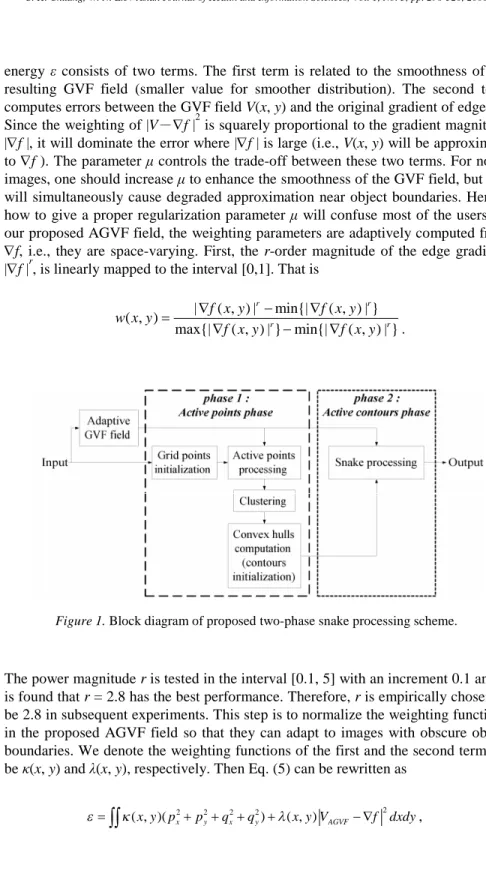
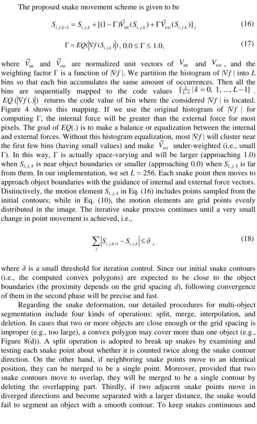
V~ are normalized unit vectors of Vint and Vext, and the weighting factor Γis a function of |f |. We partition the histogram of |f | into L bins so that each bin accumulates the same amount of occurrences. Then all the bins are sequentially mapped to the code values {Lk1|k0, 1, ...,L1} .
) (.) ( f
EQ returns the code value of bin where the considered |f | is located.
Figure 4 shows this mapping. If we use the original histogram of |f | for computing Γ, the internal force will be greater than the external force for most pixels. The goal of EQ(.) is to make a balance or equalization between the internal and external forces. Without this histogram equalization, most |f | will cluster near the first few bins (having small values) and make ext
V~ under-weighted (i.e., small Γ). In this way, Γis actually space-varying and will be larger (approaching 1.0) when Si, j, kis near object boundaries or smaller (approaching 0.0) when Si, j, kis far from them. In our implementation, we set L = 256. Each snake point then moves to approach object boundaries with the guidance of internal and external force vectors.
Distinctively, the motion element Si, j, kin Eq. (16) includes points sampled from the initial contours; while in Eq. (10), the motion elements are grid points evenly distributed in the image. The iterative snake process continues until a very small change in point movement is achieved, i.e.,
, , 1 , ,
i j k i j k
j
S S
, (18)where δis a small threshold for iteration control. Since our initial snake contours (i.e., the computed convex polygons) are expected to be close to the object boundaries (the proximity depends on the grid spacing d), following convergence of them in the second phase will be precise and fast.
Regarding the snake deformation, our detailed procedures for multi-object segmentation include four kinds of operations: split, merge, interpolation, and deletion. In cases that two or more objects are close enough or the grid spacing is improper (e.g., too large), a convex polygon may cover more than one object (e.g., Figure 8(d)). A split operation is adopted to break up snakes by examining and testing each snake point about whether it is counted twice along the snake contour direction. On the other hand, if neighboring snake points move to an identical position, they can be merged to be a single point. Moreover, provided that two snake contours move to overlap, they will be merged to be a single contour by deleting the overlapping part. Thirdly, if two adjacent snake points move in diverged directions and become separated with a larger distance, the snake would fail to segment an object with a smooth contour. To keep snakes continuous and
smooth, interpolation is applied to insert additional contour points. The condition is that if |Si, j, k-Si, j-1, k| ≥2 is satisfied, a new point Si j k, , 12(Si j k, , Si j,1,k) is inserted and the point indices are re-ordered. Besides, in cases that two non-adjacent snake points meet together or are disordered, a small loop may be formed. An interception point should be also detected to split the snake into two parts. After that, we delete short loops whose length is smaller than a threshold.
Furthermore, if a snake contains an incomplete object (e.g., Figure 8(d)) or noise, it will degenerate to an open curve or, extremely, a single point.
The computational complexity of our snake algorithm is then O(n) and faster than O(n2) of the traditional snake algorithm (Kass et al., 1988) and O(nh) of the previously proposed greedy snake (Williams & Shah 1992), where n is the number of points in the snake contour and h is the number of neighborhoods to be searched in each iteration, i.e. h=8 in Williams & Shah (1992) and h=4 in Lam and Yan (1994a).
(a) (b)
Figure 4. Histograms of (a) |f | (linearly mapped to [0,1.0]) and (b) EQ(|f |) (L=256;
equally mapped to [0,1.0]).
4. EXPERIMENTAL RESULTS
4.1. Criteria for Evaluation
Performance evaluation will be established on the average distance to the true object boundaries for each snake pixel. First, the manually segmented object boundary (e.g., the black circle in Figure 5(b)) is obtained as the reference. We assume that there are m and n contour points in the reference and computed snakes, respectively. Each contour point piin the computed snake will search for a contour point q(i) with the minimal distance in the reference snake. The average of these
to the reference one. Similarly, every contour point qjin the reference snake will search for a contour point p(j)with the minimal distance in the computed snake. We can calculate another error value er→cfor the reference snake with respect to the computed one. The average of ec→rand er→c and the maximal error that has ever occurred are used to evaluate the result of segmentation (i.e., the computed snakes).
These equations are
( ) ( )
avg
1{ }
2 2
i j i j
c r r c i j
q p p q
e e
error
n m
(19)
and
( ) ( )
max max{max( i i ), max( j j )}
i j
error p q q p
. (20)
4.2. Analysis of the AGVF Field
To make a performance comparison between the proposed AGVF and traditional GVF (Xu & Prince, 1998) fields, we create a series of noisy images, whose signal-to-noise ratios (SNRs) are from 14.6 dB down to 4.7 dB, for testing.
In this part of experiments, the active-points phase is not employed and the initial snake contours are manually provided so as to clarify the performance difference between these two GVF fields. Since the traditional GVF field is stable only with the Courant-Friedrichs-Lewy step-size restriction (Xu & Prince, 1998), the regularization parameter μwill be restricted to be within 0~0.25.
Figure 5(a)demonstratesa“circle”imagecorrupted with Gaussian random noise and Figure 5(b) shows its edge map obtained by gradient operation. In Figure 5(b), two concentric circles, the white one as the initial snake contour and the black one as the reference contour for comparison, are superimposed. In traditional snake model (Eq. (4)), the weighting parameters are set with α= 0.05, β= 0, γ= 0.6.
Figures 5(c) through 5(g) show the results of snake processing by using GVF fields of different μvalues ( μ= 0.01~0.25) and Figure 5(h) shows the snake result by using our AGVF field. It can be found that most of the GVF fields, except the one obtained with μ= 0.25, produce inferior detection of object boundaries than our proposed AGVF field.
Figures 6(a) and 6(b) plot the curves presenting the relation between μand segmentation errors (as defined in Section 4.1) in images of different SNRs. Here, μ is extended to 0.3 to show the instability of traditional GVF field when μ> 0.25. In Figure 6, the solid lines are curves of errors resulting from traditional GVF fields, while the dotted ones represent errors (independent of μ) resulting from the AGVF field. The upper curves of both kinds represent the maximal errors evaluated by using Eq. (20) and the lower curves are average errors by using Eq. (19). The
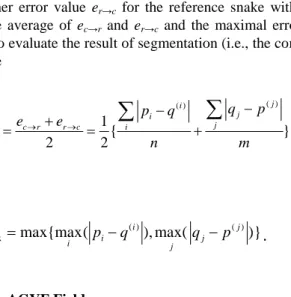
proposed AGVF field leads to errors of (1.0, 0.5) pixels and (0.9, 0.4) pixels for images of SNRs equal to 14.6 dB and 4.7 dB, respectively. It can be found that for images of high SNRs, e.g., Figure 6(a), a broader range of μis allowable (where errors are small) for traditional GVF field. When the images are noisy, e.g., Figure 6(b), the acceptable range of μis narrowed down and even located beyond μ= 0.25.
Contrarily, even though the images are much noisier, our AGVF field can still provide good attracting forces and result in small segmentation errors. Figures 6(c) and 6(d) show curves that represent relationships between SNRs and errors at different μ(0.01 and 0.25). It can be found that a small μ(e.g., 0.01) is hardly suitable to all range of SNRs (down to 4.7 dB). When μis increased up to 0.25, e.g., Figure 6(d), the resulting GVF field leads to a better segmentation but is still unsatisfactory for noisy images with SNRs smaller than 5 dB.
Obviously, there is a trade-off between choosing a small or large μvalue. For images of higher SNRs, more stress could be placed on the approximation of the GVF field to f (i.e., low μ). When the images are noisy, smoothness of the computed GVF field should be stressed (i.e., high μ) so that segmentation errors can be reduced. On the other hand, our AGVF field provides this trade-off automatically. It can achieve a uniform and stable performance (a maximal error of about 1.0 pixel and an average error of about 0.5 pixel) in a broad range of SNRs (4.7~14.6 dB).
(a) (b) (c) (d)
(e) (f) (g) (h)
Figure 5. (a) Original image (SNR= 5.0 dB); (b) edge map of (a) superimposed with initial (white circle) and reference (black circle) contours; (c)–(g) resultant snakes (the white curves) by using traditional GVF fields with μ= 0.05, 0.1, 0.15, 0.2, 0.25, respectively; (h) resultant snake by using our proposed AGVF field.
(a) (b)
(c) (d)
Figure 6. (a)–(b) Relations of errors (maximum and average) vs. μat different SNRs (14.6 dB and 4.7 dB); (c)–(d) relations of errors (maximum and average) vs. SNR at different μ(0.01 and 0.25).
4.3 Experiments of Proposed Two-Phase Snake Processing Scheme
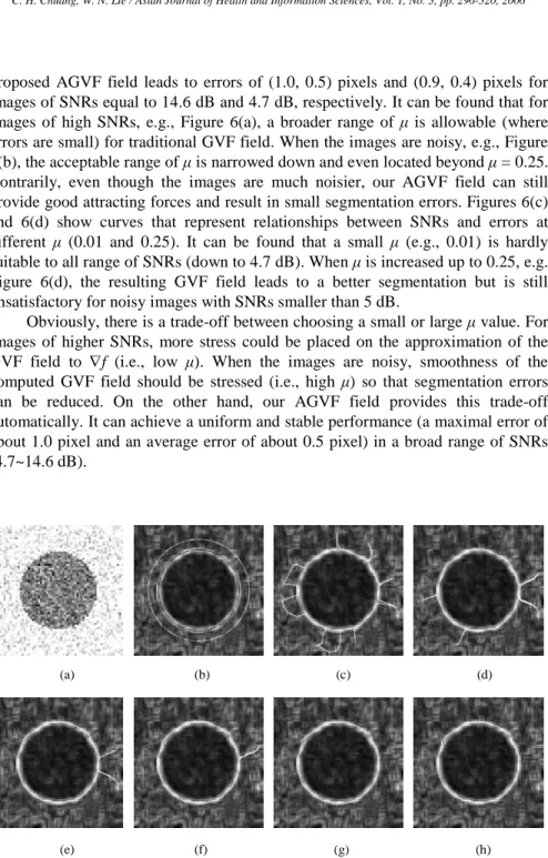
Wefirstexperimentwith aseriesofartificial“Annulus”images(256256 pixels) corrupted with noise. Intensities of the background and annulus areas are added with different amounts of Gaussian noise so that the SNRs are 13.60, 10.64, 6.93, 4.46, and 2.51 dB, respectively. Accordingly the grid spacings for initial active points are chosen to be 8, 8, 6, 4, and 4-pixel, respectively, which are fine enough to distinguish two concentric circle boundaries (an image with a smaller SNR should have a smaller grid spacing). After several processing iterations, the converged active points are then grouped into two clusters (the inner and outer rings), from which the minimum enclosing polygons can be figured out and adopted as the initial snake contours. Figure 7(b) demonstrates the result of Figure 7(a) (SNR = 2.51 dB) after active-points processing with a deliberately larger clustering distance threshold dthd. We perform, in the following active-contours phase, the greedy (Williams & Shah, 1992) and traditional GVF snake (Xu &
Prince, 1998) for comparison. The weighting parameters (α, β, γ) are set with (0.5,
0.5, 1.0) (for greedy) and (0.1, 0.3, 0.6) (for GVF), respectively. Figures 7(c) through 7(e) give the final snake contours by the greedy, traditional GVF, and our proposed algorithms, where the maximal errors are 15.61, 6.00, and 3.92 pixels and the mean errors are 1.74, 1.41, and 1.22 pixels, respectively. The result convinces us that even with a high noise (SNR = 2.51 dB) or a far initial snake, our method can faithfully extract the boundaries of the annulus. The CPU time spent for the three snake algorithms is about 0.01, 0.05, and 0.01 sec on a Pentium III 1G Hz processor (the minimum computing time unit is 0.01 sec), respectively. Figures 7(f) and 7(g) plot the curves of the maximal and mean errors vs. SNRs, respectively, for the initial snake contour and the outputs of the three snake algorithms. Note that the convergence of snakes, especially the greedy snake, is certainly affected by the positions of initial contours.
For applications to real images, we use biomedical (Figures 8–10) and military (Figures 11 and 12) images for simulations. Figure 8 shows the experiment for human blood cells. Considering possible proximity between cells, the grid spacing is set to 2 pixels only (Figure 8(b)). Figure 8(c) shows the converged active points around boundaries of cells. They are grouped into 4 major clusters and result in 4 initial snakes (those enclosing complete cells) as shown in Figure 8(d). Figures 8(e) through 8(g) show the snake results by using the greedy, traditional GVF, and proposed algorithms. Although one of the initial snakes contains three cells, they can be separated successfully by our method, but not by the greedy and the traditional GVF snakes. For noisy dots and incomplete cells around the image border, our algorithm rejects them without any by-product effects. Figure 9 shows the experiment for frog blood cells. The grid spacing is 6 pixels, leading to less time spent (about 0.06 sec) in the active-points process (Figures 9(b)–9(d)). Some artifacts occur in the results by using the greedy and the traditional GVF snakes, as shown in Figures 9(e) and 9(f). Another experiment (Figure 10) shows the robustness of the proposed algorithm in segmenting ventricles in CT brain images.
Although the boundary between the ventricle and the brain tissue is fuzzy, the target ventricle is enclosed successfully by active-points processing (Figures 10(b)–10(d)) and segmented approximately by active-contours processing (Figure 10(g)). Obviously, the greedy snake cannot approach the heavily concave part of the ventricle (Figure 10(e)) and the traditional GVF snake is easily trapped into local minima due to possibly improper weighting parameters (Figure 10(f)).
Figures11 and 12 show experimentsforthe“Truck”and “Multiplecars”images. Although many active points are caught by the brakes (Figures 11(b) and 12(b)), they are scattered and can be removed by a threshold number of clustered active points (i.e., nthdin Section 3.2), as shown in Figures 11(c) and 12(c). In these two cases, though the objects are located in noisy surroundings, our algorithm still outperforms others and gives satisfactory results. Table 1 compares the traditional snake, greedy snake, GVF snake, and proposed two-phase AGVF snake in several aspects to show the superiority of our algorithm.
(a) (b) (c)
(d) (e)
(f) (g)
Figure 7.Performancecomparison of“Annulus”imageswith varying SNRs. (a) Original image corrupted by noise (SNR = 2.51 dB), (b) initial snake curves after active-points processing with a deliberately larger clustering distance dthd, (c) greedy snake result (α= 0.5, β= 0.5, and γ= 1.0), (d) traditional GVF snake result (α= 0.1, β= 0.3, and γ= 0.6), (e) proposed snake result, (f) maximal error vs. SNR, (g) mean error vs. SNR.
(a) (b) (c) (d)
(e) (f) (g)
Figure 8. Experiments for the “human blood cells”image. (a) Original image (170156 pixels), (b) initial grid active points, (c) converged active points, (d) result of active-points phase (initial snakes), (e) result of greedy snake (α= 0.5, β= 0.5, and γ= 1.0), (f) result of traditional GVF snake (α= 0.1, β= 0.3, and γ= 0.6), (g) result of proposed snake.
(a) (b) (c)
(d) (e) (f) (g)
Figure 9.Experimentsforthe‘frog blood cells’image.(a)Originalimage(240190 pixels), (b) initial grid active points, (c) converged active points, (d) result of active-points phase (initial snakes), (e) result of greedy snake (α= 0.5, β= 0.5, and γ= 1.0), (f) result of traditional GVF snake (α= 0.1, β= 0.3, and γ= 0.6), (g) result of proposed snake.
(a) (b)
(c) (d)
(e) (f) (g)
Figure 10. Experimentsforthe‘Brain’CT image.(a)Originalimage(130140 pixels), (b) initial grid active points, (c) converged active points, (d) result of active-points phase (initial snakes), (e) result of greedy snake (α= 0.5, β= 0.5, and γ= 1.0), (f) result of traditional GVF snake (α= 0.1, β= 0.3, and γ= 0.6), (g) result of proposed snake.
(a) (b)
(c) (d)
(e) (f)
Figure 11.Experimentsforthe ‘Truck’image. (a) Original image (256256 pixels), (b) converged active points, (c) result of active-points phase (initial snakes) (dthd= 12 pixels, nthd= 15 points), (d) result of greedy snake (α= 0.5, β= 0.5, and γ= 1.0), (e) result of traditional GVF snake (α= 0.1, β= 0.3, and γ= 0.6), (f) result of proposed snake.
(a) (b)
(c) (d)
(e) (f)
Figure 12.Experimentsforthe‘Multiplecars’image.(a)Originalimage (256256 pixels), (b) converged active points, (c) result of active-points phase (initial snakes) (dthd
= 9 pixels, nthd= 15 points), (d) result of greedy snake (α= 0.5, β= 0.5, and γ=
1.0), (e) result of traditional GVF snake (α= 0.1, β= 0.3, and γ= 0.6), (f) result of proposed snake.
Table 1. A comparison of four kinds of snake algorithms for multi-object segmentation
Traditional snake Greedy snake Traditional GVF snake
Proposed two-phase AGVF snake
GVF field No No Yes Yes (Adaptive)
Snake initialization Manual Manual Manual Automatic
Noise resistance Low Low High High
Weighting parameters in snake model
Manual and fixed Manual and fixed Manual and fixed Space-varying or Adaptive
Snake movement search Yes (Global) Yes (Local) Yes (Global) No
Object segmentation Single Single Single Multiple
5. CONCLUSIONS AND REMARKS
In this research, a new automatic two-phase snake algorithm for segmenting multiple objects is proposed. The “automatic”comes from the distribution of grid active-points over the entire image so as to determine the initial snake contours at proper positions without manual interaction. Our algorithm is also capable of segmenting multiple or annular objects (more versatile than traditional snake algorithms). All processing is based on our proposed AGVF field which adopts space-varying weighting functions to provide a stable and uniform performance over a broad range of image SNRs. In the active-contours phase, a no-search strategy is adopted so as to increase processing speed and efficiency. The snake points move with the guidance of internal and external forces which are computed directly from the current snake contour status and AGVF vectors, respectively.
Hence, neither global nor local evaluation of the next movement is required.
One disadvantage of the GVF-based algorithm is that the GVF/AGVF fields must be obtained prior to snake deformation and it actually spends most CPU time, e.g., about 2 seconds on a Pentium III 1G Hz processor for a 256×256 image.
Fortunately, a multi-resolution GVF computing architecture has been recently proposed (Ntalianis, Doulamis, Doulamis, & Kollias, 2001) to speed up the computation significantly by nearly 40 times. Our two-phase AGVF snake processing can make use of a 2-level AGVF field to further improve the speed and efficiency.
The proposed algorithm will be versatile anywhere automatic detection or segmentation of multiple objects is required, e.g., in an image retrieval system and biomedical image processing and analysis.
REFERENCES
Chuang, C. H., & Lie, W. N. (2001). Automatic snake contours for the segmentation of multiple objects. Proceedings of IEEE International Symposium on Circuits and Systems II, Sydney, Australia, 389-392.
Davison, N. E., Eviatar, H., & Somorjai, R. L. (2000). Snakes simplified. Pattern Recognition, 33(10), 1651-1664.
Deng, J., & Tsui, H. T. (2002). A fast level set method for segmentation of low contrast noisy biomedical images. Pattern Recognition Letters, 23(1-3), 161-169.
Ji, L., & Yan, H. (2002a). Attractable snakes based on the greedy algorithm for contour extraction. Pattern Recognition, 35(4), 791-806.
Ji, L., & Yan, H. (2002b). Robust topology-adaptive snakes for image segmentation. Image and Vision Computing, 20, 147-164.
Kang, D. J. (1999). A fast and stable snake algorithm for medical images. Pattern Recognition Letters, 20(5), 507-512.
Kass, M., Witkin, A., & Terzopoulos, D. (1988). Snakes: active contour models.
International Journal of Computer Vision, 1(4), 321-331.
Lam, C. L., & Yuen, S. Y. (1998). An unbiased active contour algorithm for object tracking. Pattern Recognition Letters, 19(5-6), 491-498.
Lam, K. M. & Yan, H. (1994a). Fast greedy algorithm for active contours.
Electronics Letters, 30(1), 21-23.
Lam, K. M., & Yan, H. (1994b). Locating head boundary by snakes. Proceedings, International Symposium on Speech, Image Processing and Neural Networks, (ISSIPNN’94), Hong Kong, China, 17-20.
Lie, W. N., & Chuang, C. H. (2001). A fast and accurate snake model for object contour detection. Electronics Letters, 37(10), 624-626.
Looney, C. G. (1997). Pattern recognition using neural networks. New York, USA:
Oxford University Press.
Matsuda, Y., Sumi, Y., Kataoka, D., Ota, M., Yabuki, N., Fukui, Y., & Miki, S.
(2000). Proposal for a convergence criterion to the active net in two steps.
Proceedings of IEEE International Symposium on Circuits and Systems, Geneva, Switzerland, 313-316.
Mirhosseini, A. R., & Yan, H. (1997). An optimally fast greedy algorithm for active contours. Proceedings of IEEE International Symposium on Circuits and Systems, Hong Kong, China, 1189-1192.
Ntalianis, K. S., Doulamis, N. D., Doulamis, A. D., & Kollias, S. D. (2001).
Multiresolution gradient vector flow field: a fast implementation towards video object plane segmentation. Proceedings of IEEE International Conference on Multimedia and Expo, Tokyo, Japan, 1-4.
Osher, S., & Fedkiw, R. P. (2001). Level set methods: an overview and some recent results. Journal of Computational Physics, 169(2), 463-502.
Pardo, J. M., Cabello, D., & Heras, J. (1997). A snake for model-based segmentation of biomedical images. Pattern Recognition Letters, 18(14), 1529-1538.
Pardo, X. M., & Cabello, D. (2000). Biomedical active segmentation guided by edge saliency. Pattern Recognition Letters, 21(6-7), 559-572.
Park, J., & Keller, J. M. (2001). Snakes on the watershed. IEEE Transactions on Pattern Analysis and Machine Intelligence, 23(10), 1201-1205.
Precioso, F., & Barlaud, M. (2002). B-spline active contour with handling of topology changes for fast video segmentation. EURASIP Journal on Applied Signal Processing, 6, 555-560.
Sonka, M., Hlavac, V., & Boyle, R. (1999). Image processing, analysis, and machine vision. Pacific Grove, California, USA: Brooks/Cole, 228-289.
Velasco, F. A., & Marroquin, J. L. (2003). Growing snakes: active contours for complex topologies. Pattern Recognition, 36(2), 475-482.
Williams, D. J., & Shah, M. (1992). A fast algorithm for active contours and curvature estimation. CVGIP: Image Understanding, 55(1), 14-26.
Wong, Y. Y., Yuen, P. C., & Tong, C. S. (1998a). Contour length terminating criterion for snake model. Pattern Recognition, 31(5), 597-606.
Wong, Y. Y., Yuen, P. C., & Tong, C. S. (1998b). Segmented snake for contour detection. Pattern Recognition, 31(11), 1669-1679.
Xu, C., & Prince, J. L. (1998). Snakes, shapes, and gradient vector flow. IEEE Trans. Image Processing, 7(3), 359-369.
Yuen, P. C., Wong, Y. Y., & Tong, C. S. (1996). Contour detection using enhanced snakes algorithm. Electronics Letters, 32(3), 202-204.
Yuen, P. C., Feng, G. C., & Zhou, J. P. (1999). A contour detection method:
initialization and contour model. Pattern Recognition Letters, 20(2), 141-148.
Cheng-Hung Chuang received a B.S. degree in electrical engineering from Tatung Institute of Technology, Taiwan, in 1994, and M.S. and Ph.D. degrees in electrical engineering from National Chung Cheng University, Taiwan, in 1996 and 2003, respectively. From 2003 to 2007, he was a member of the Institute of Statistical Science, Academia Sinica, Taipei, Taiwan, as a postdoctoral fellow for human brain science research. In Feb. 2007, he entered the Department of Computer Science and Information Engineering, Asia University, Taiwan, as an assistant professor. His research interests include image/video processing, optical and biomedical signal processing, 3-D display systems, computer vision, and pattern recognition.
Wen-Nung Lie was born in Tainan, Taiwan, R. O.
C., in 1962. He received B.S., M.S., and Ph.D. degrees, all in electrical engineering, from National Tsing Hua University, Taiwan, R. O. C., in 1984, 1986, and 1990, respectively. From September 1990 to June 1996, he served as an assistant scientist in Chung Shan Institute of Science and Technology (CSIST), Taiwan, R. O. C., where he was devoted to the development of an infrared imaging system and target tracker for military applications.
In August 1996, he joined the Department of Electrical Engineering, National Chung Cheng University, Taiwan, R. O. C., as an associate professor. From July 2000 to Jan. 2001, he was a visiting scholar in the University of Washington, Seattle, WA, USA. His research interests include image/video compression, networked video transmission, audio/image/video watermarking, multimedia content analysis, standard-compliant multimedia encryption, infrared image processing, 3-D stereo virtual reality by image-based rendering, and industrial inspection by computer vision techniques.
![Figure 4. Histograms of (a) |f | (linearly mapped to [0,1.0]) and (b) EQ(|f |) (L=256;](https://thumb-ap.123doks.com/thumbv2/9libinfo/9502831.596408/12.774.154.624.452.655/figure-histograms-f-linearly-mapped-b-eq-l.webp)