景氣循環、通貨膨脹衡量及聯邦資金利率期貨三論

國立臺灣大學 經濟學系 博士論文

景氣循環、通貨膨脹衡量及聯邦資金利率期貨三論

顏承暉

撰

99/2

國立臺灣大學社會科學學院經濟學系 博士論文

Department of Economics College of Social Sciences

National Taiwan University Doctoral Dissertation

景氣循環、通貨膨脹衡量及聯邦資金利率期貨三論 Three Essays on Business Cycles,

Inflation Measurement and Fed Funds Rate Futures

顏承暉 Chen-Hui Yen

指導教授﹕梁國源 教授

Advisor: Kuo-Yuan Liang, Professor.

中華民國 99 年 2 月

February, 2010

To my dear family, Julie and good friends:

Thanks for your support and encouragement in my student career.

To dear Prof. Liang, Prof. Chou and committee members:

Your guidance and comments contributes this dissertation.

Yen, Chen-Hui February, 2010

中文摘要

研究總體時間序列資料並據以提供其實務上的應用及意涵是總體經濟學家的 重要工作。然而，和其他領域實證研究相較，景氣循環在投資組合上的應用、

Kitchin、Juglar 以及 Kuznets 循環間的交互作用、通貨膨脹衡量以及聯邦資金利率 期貨對美國貨幣政策的預測能力等方面的研究在文獻中屬於相對少數。基於此原 因，本論文將針對這些實務上重要的總體經濟議題從實證的角度分析，並據此提 出其意涵。

本論文第一章應用頻譜分析（spectral analysis）來探討景氣循環以及資產價格 的循環現象。第一節將介紹頻譜分析如何應用在景氣循環研究上。第二節則探討 景氣循環對不同類別資產價格的意涵。首先，本節將利用 Canova (1996)所提出的 檢定方法驗證債券市場、股票市場、商品市場是不是具有相似的循環現象。其次，

本節還應用 Fuller (1996)的檢定方法，透過交叉頻譜分析驗證各資產價格與景氣循 環的領先落後關係。研究顯示：(1) 債券、股票以及商品市場具有和景氣循環相似 的循環週期，週期介在 3.5~7.5 年間；(2)債券、股票、景氣循環以及商品市場間存 在四個具統計上顯著的領先或落後的關係：分別是景氣循環領先商品市場，然而 卻同時落後債券市場以及股票市場，又債券市場領先商品市場。此外，本節還透 過實際的資料指出，應用這樣的領先落後關係，在不同景氣循環階段持有相對強 勢的資產類別，有助於增加投資組合的獲利。

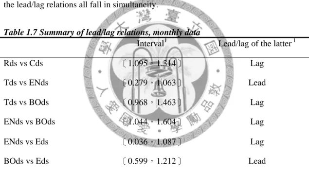
第三節則更進一步分析九大類的共同基金報酬是否也具備有循環上的關連 性。研究結果指出：(1) 不同種類的基金類別的確也存在類似的循環現象；(2) 其 中存在三種領先或落後的關係，分別是債券型基金領先股票型基金、股票型基金 領先能源型基金；債券型基金領先科技型基金、科技型基金領先能源型基金；貨 幣型基金領先地產型基金。

第四節將利用 1870 至 2008 年 15 個 OECD 國家的資料，並應用 Canova (1996) 所提出的檢定方法證明，除了大家所熟悉的 3~5 年 Kitchin 循環外，這段期間大多 數的 OECD 國家同時也經歷具有規律性的 7~11 年之 Juglar 循環，以及 15~25 年的 Kuznets 循環。除此之外，本節還比對歷次 OECD 所認定的景氣循環高峰與谷底日 期以及其所處 Juglar 循環以及 Kuznets 循環的該當階段發現，當經濟同時處於 Juglar

及 Kuznets 循環的上升階段時，OECD 所認定的循環擴張期通常會比較長。而當經 濟同時處於 Juglar 及 Kuznets 循環的下降階段時，OECD 所認定的短循環景氣收縮 期通常會較長。值得注意的是，這一節還指出 Kitchin、Juglar 及 Kuznets 循環同時 進入收縮期是造成 1930 年經濟大蕭條以及 2008 年全球金融海嘯的共同原因之一。

鑑於通貨膨脹是總體經濟學的重要議題，而近年來各電子及平面媒體經常出 現官方公布之通貨膨脹與一般民眾生活經驗顯不相當的輿論。因此本論文的第二 章將探討如何衡量消費者物價指數（CPI）的可靠度。本章試圖建構一個新的迴歸 模型，透過模型的估計結果來衡量 CPI 的可靠性。更進一步來說，該模型是文獻 上指數隨機方法（the stochastic approach to index numbers）的擴充。本文認為，傳 統上的指數隨機方法中關於相對價格間系統性改變的機制應該要隨時間作改變。

因此，在這一章的模型中，將加入一般通貨膨脹率以及景氣循環階段等虛擬變數 來解決文獻上的不足。而這樣的延伸也更能夠回答凱因斯對於指數隨機方法的批 判。此外，本章還應用澳洲以及美國的資料，比對本論文與傳統設定方法的實證 差別，結果顯示，這一章的設定較傳統的方法更合適用來衡量 CPI 的可靠度。

聯邦資金利率期貨是否具有未來聯邦資金利率走勢的預測能力是文獻上重要 的議題之一，然而過去的研究對於這個議題大多以量化的預測能力來衡量，對於 質化（方向性）預測能力的討論則相對有限。但從 1989 年起聯邦資金利率的變動 即以 0.25%及其倍數的幅度調整，因此傳統文獻上的量化預測能力評估並不適當。

有鑑於此，本論文第三章將應用 Pesaran 及 Timmermann (1992, 1994)所提出的無母 數一般化 Henriksson-Merton (H-M)檢定驗證聯邦資金利率期貨對未來聯邦資金利 率走向是否具有方向性預測能力。主要實證結果表明，聯邦資金利率期貨對於 (1) 貨幣政策緊縮、寬鬆或中立，或(2)目前貨幣政策升息或降息循環的轉折點至少在 1 週之前就具有預測能力。此外，本章亦驗證，隨著 1994 年 2 月美國貨幣政策制定 過程更趨透明化，聯邦資金利率期貨的預測能力是否有所改善。結果顯示，利率 期貨的預測能力的確隨著聯準會政策制定過程的更為透明化而有所增進。

關鍵字：景氣循環、投資組合管理、頻譜分析、指數隨機方法、聯邦資金利率期 貨、方向性預測準確性

英文摘要

Macroeconomists carry the duty of providing insights and creating application value for practitioners based on studying macroeconomic time series data. However, compared with empirical studies in other areas, application of the business cycle concept on investment portfolios, the interplay between the Kitchin, Juglar and Kuznets cycles, the measurement of inflation rates, and the predictability of Fed Funds futures on U.S.

monetary policy are all relatively underrepresented in literature. To bridge the gap in literature, this dissertation aims to study these practically important issues with a formal statistical procedure.

The first chapter applies the spectral analysis to discuss the cyclical patterns of business cycles and asset prices. Section 1 briefly introduces the application of spectral analysis on the study of business cycles. Section 2 uses spectral analysis to discuss the implication of the business cycle concept on the investment of multiple asset classes. In this section, Canova’s (1996) test is applied to test whether if the bonds market, stock market and commodities market have similar cyclical features as the business cycle.

Moreover, the test in Fuller (1996) is applied to verify if lead or lag relationships exist between asset prices of the three markets, respectively, and the business cycle with cross spectrum analysis. Empirical results indicate that (1) Bond, stock and commodity markets all have similar cyclical patterns as the business cycles, which are about 3.5~7.5 years in length. (2) There are four statistically significant pairs of lead or lag relationships among the bonds, stocks and commodities market, respectively, and the business cycle, they are: the business cycle leads the commodities market, and lags both the bonds market and stock market, respectively, and the bonds market leads the commodities market. In addition, we have verified through actual data that applying

such lead or lag relationship to hold the relative stronger asset class in each corresponding phase of the business cycle can help improve the returns of a portfolio.

Then, section 3 analyzes whether 9 types of mutual funds also possess similar connections in their cyclical patterns. Empirical results indicate that (1) These mutual fund types exhibit similar cyclical patterns. (2) Among them, there are three types of lead or lag relationships, in which bond funds lead stock market funds, stock market funds lead energy funds; bond funds lead technology funds, technology funds lead energy funds; and money market funds lead real estate funds.

Section 4 uses data from 15 OECD countries from 1870 thru 2008 and apply Canova’s (1996) test to prove that, other than the well recognized 3~5 year Kitchin cycle, most OECD countries have experienced regular 7~11 year Juglar cycles and 15~25 year Kuznets cycles as well during the same period. In addition, as we compare the business cycle peaks and troughs dates recognized by the OECD with the Juglar cycle and Kuznets cycle patterns identified in our model, we found that when the economy is in the upswing of Juglar and Kuznets cycles, the expansions of the short cycle identified by the OECD are usually longer. Also, when the economy is in the downswing of Juglar and Kuznets cycles, the contractions of the short cycle identified by the OECD are usually longer. This section further points out that the joint downswing of the Kitchin, Juglar and Kuznets cycle is one of the common causes of the 1930 Great Depression and the 2008 global financial crisis.

Inflation has always been a core issue in macroeconomics. Recent media highlighted the issue that the official inflation rates may not match public experience.

Therefore in Chapter II, we shall discuss the measurement of the reliability of CPI. Here we try to construct a new regression model that can measure the reliability of CPI, which model is an extension of the stochastic approach to index numbers. Therefore,

the mechanism of systematic change in relative prices in the literature of stochastic approach to index numbers is allowed to vary with time in this chapter. Then we included inflation rate and phases of business cycle dummies in our model to allow for time varying. Such an extension can answer the Keynes’s critic on stochastic approach to index numbers. Moreover, we used US and Australian data, and compared the results from our setting with those from the traditional setting, and further confirmed that our setting was more appropriate than the conventional.

Whether the Fed Funds rate futures have the ability to predict future Fed Funds rates is a significant issue in literature. However, most past research evaluates predictive ability with quantitative measurements, while its qualitative (directional) accuracy was less emphasized. Since changes in Fed Funds rates were in multiples of 0.25% since 1989, therefore the quantitative evaluation used in traditional literature may not be adequate. Hence in Chapter III, the non-parametric generalized Henriksson-Merton (H-M) test proposed by Pesaran and Timmermann (1992, 1994) is applied to verify the directional predictive ability of FF futures on FF rates. The major empirical results are (1) predicting the tightening, easing, or maintaining of monetary policy (2) when the monetary policy reaches a probable turning point, the futures based predictors are reliable for at least one week. In this chapter, we also investigate the effects of practice changes of the US monetary policy process made in February 1994.

The results show that the reliability of futures based predictors have improved since then, which was marked a time when the FOMC decisions were made more open and transparent.

Keywords: Business cycles, portfolio management, spectral analysis, stochastic

approach to index numbers, Fed Funds futures, directional forecasting accuracy

目 錄

口試委員會審定書 ... I 誌謝 ...II 中文摘要 ... III 英文摘要 ...V 目 錄 ...VIII 圖目錄 ... XI 表目錄 ...XII

Introduction ... 1

Chapter 1 Dissecting of Business Cycles: Applications of Spectral Analysis ... 4

I. Introduction to the Spectral Analysis on Analyzing Business Cycle... 4

1.1 Introduction ... 4

1.2 Univariate Spectral Analysis ... 5

1.2.1 Detrending and Signal Extraction ... 5

1.2.2 Testing for Business Cycle... 8

1.3 Multivariate Spectral Analysis ... 9

II. An Intermarket Investigation and its Implications to Portfolio Reallocation ... 11

2.1 Introduction... 11

2.2 A Review of Earlier Studies... 13

2.2.1 The Relationship between Different Asset Prices and the Business Cycle 13 2.2.2 The Applicability of Intermarket Framework... 15

2.3 Rationales and Empirical Verification of the Existence of Intermarket Relationships... 17

2.3.1 Rationales of the intermarket relationships ... 17

2.3.2 Data... 20

2.3.3 The existence of cyclical behavior ... 21

2.3.4 Lead-lag relationship between markets ... 23

2.4 Portfolio Return within Business Cycles ... 26

2.5 Conclusions and Remarks... 31

III. Cycle and Performance of Mutual Funds. ... 33

3.1 Introduction... 33

3.2 Data and methodology ... 33

3.2.1 Data... 33

3.2.2 Uni-spectral analysis ... 34

3.2.3 Cross-spectral analysis ... 35

3.3 Empirical results ... 36

IV. Interplay among Business Cycles Reconsidered: Implications for the 2008 Global Recession. ... 40

4.1 Introduction ... 40

4.2 Early Inquiry of Interplay Between Business Cycles ... 41

4.3 Data ... 45

4.4 The Existence of Kitchin, Juglar, and Kuznets Cycles ... 47

4.5 Phases of the Kitchin, Juglar, Kuznets, and Kondratieff Cycle ... 51

4.5.1 Interplay Between Business Cycles ... 51

4.5.2 Experience in the Great Depression and this Time Recession ... 56

4.6. Concluding Remarks... 59

Appendix 1.1 ... 60

Chapter 2 Measuring CPI’s Reliability: the Stochastic Approach to Index Numbers Revisited... 64

I. Introduction ... 64

II Brief Introduction of Stochastic Approach to Index Numbers... 67

III Specification of the Full model ... 72

IV Empirical Evidence ... 75

V Concluding Remarks ... 84

Appendix 2.1: Estimated Standard Errors of CPI of Australia and US by Crompton’s Method... 85

Appendix 2.2: Estimated Standard Errors of CPI of Australia and US by Adding Economic Environment Dummies ... 87

Chapter 3 An Application of Henriksson-Merton Test: Are Fed Funds Rate Futures Valuable in Predicting US Monetary Policy? ... 89

I. Introduction... 89

II. A Review of Earlier Studies... 92

2.1. Rationality Testing and Forecasting Accuracy Evaluation... 92

2.2. Importance of Directional Accuracy... 93

2.3. Monetary Policy Cycle... 94

2.4. Changes in FOMC Disclosure Practices ... 94

III. Silent Features of the FF Future Rate ... 96

IV. Usefulness of Futures for Predicting Fed Funds Rate... 98

V. Concluding Remarks ... 104

Appendix 3.1. Contingency tables regarding “tighten, ease or unchanged”... 105

Appendix 3.2. Contingency tables regarding the turning point of the monetary policy cycle ... 108

References ... 111

圖目錄

Figure 1.1 An idealized diagram of how bond, stock and commodity interact during a

typical business cycle ... 12

Figure 1.2 Spectral density, S&P500, 10 years gov. bond, RJ/CRB, industrial production ... 22

Figure 1.3 Filtered series of 10-years gov. bond, S&P 500, industrial productions and commodity futures... 24

Figure 1.4 The significant lead/lag relations between different markets ... 25

Figure 1.5 The partition of each fund for X category funds... 36

Figure 1.6 The lead/lag relations of monthly data... 39

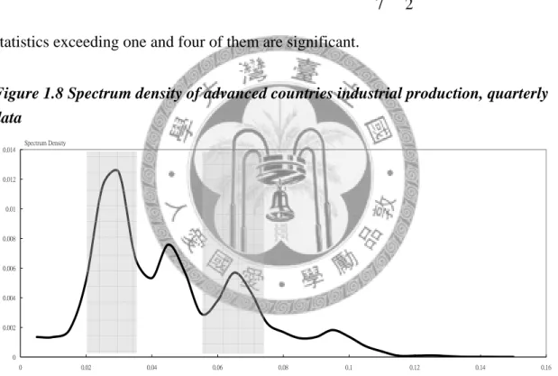
Figure 1.7 Spectrum density of aggregate GDP, yearly data... 49

Figure 1.8 Spectrum density of advanced countries industrial production, quarterly.... 50

Figure 1.9 CF-filter decomposition of World GDP cycles, 1870-2008, yearly data ... 51

Figure 1.10 CF-filter decomposition of World IP cycles, Q1/1961-Q1/2009, quarterly data ... 52

Figure 2.1 Estimated standard errors of Crompton’s method and the absolute difference values between the inflation rate at time t with general inflation mean, Australia 76 Figure 2.2 Estimated standard errors of Crompton’s method and the absolute difference value between the inflation rate at time t with the general inflation mean, US .... 77

Figure 2.3 Estimated standard errors after adding dummies and the absolute difference values between the inflation rate at time t with general inflation mean, Australia 82 Figure 2.4 Estimated standard errors after adding dummies and the absolute difference values between the inflation rate at time t with the general inflation mean, US .. 82

Figure 3.1 1995~2007 Average FF futures Open Interests... 96

Figure 3.2 Forecast and actual change of FF target rate... 100

Figure 3.3 Forecast and actual change of policy cycle turning point... 103

表目錄

Table 1.1 Univariate spectral statistic... 22

Table 1.2 Square coherence and average lead/lad time ... 25

Table 1.3 Average annual return of portfolio (May, 1960－December, 2007)... 27

Table 1.4 Portfolio return over individual business cycles... 31

Table 1.5 Numbers of funds in each category ... 34

Table 1.6 Univariate spectral statistic, monthly data... 37

Table 1.7 Summary of lead/lag relations, monthly data ... 38

Table 1.8 Canova test for short, medium and long term Cycle ... 48

Table 1.9 Matching the OECD business cycle reference dates and Kitchin cycle turning points ... 53

Table 1.10 Average duration of expansion and contraction during long cycle upturn and downturn (quarters) ... 54

Table 1.11 Nearest turning points of each cycles before the Great Depression of 1930 57 Table 1.12 Nearest turning points before the 2008 World Recession... 58

Table A.1.1 Reference business cycle date of 15 OECD countries... 60

Table 2.1 Number of months with high standard errors during different business cycle phases of Australia using Cromptom (2000)’s method ... 79

Table 2.2 Number of months with high standard errors during different business cycle phases of US using Cromptom (2000)’s method ... 79

Table 2.3 The total number of months where “high standard errors of estimated CPI” occurred in different business cycle phases in the US after adding dummies ... 83

Table 2.4 Summary statistic results before and after the inclusion of dummies ... 83

Table A.2.1 Estimated standard errors of CPI of Australia by Cromptom (2000)’s method... 85

Table A.2.2 Estimated standard errors of CPI of US by Cromptom (2000)’s method ... 86

Table A.2.3 Estimated standard errors of CPI of Australia by adding dummies... 87

Table A.2.4 Estimated standard errors of CPI of US by adding dummies ... 88

Table 3.1 Market timing statistics of FF futures rates ... 101

Table 3.2 Market timing statistics of policy cycle turning points ... 103

Table A.3.1 Forecast and actual change regarding “tighten, ease or unchanged” (full range)... 105

Table A.3.2 Forecast and actual change regarding “tighten, ease or unchanged” (pre 1994/2... 106 Table A.3.3 Forecast and actual change regarding “tighten, ease or unchanged” (after

1994/2) ... 107 Table A.3.4 Forecast and actual change of policy cycle turning point (full range)... 108 Table A.3.5 Forecast and actual change of policy cycle turning point (pre 1994/2).... 109 Table A.3.6 Forecast and actual change of policy cycle turning point (after 1994/2)...110

Introduction

Macroeconomists carry the duty of providing insights and creating application value for practitioners based on studying macroeconomic time series data. However, compared with empirical studies in other areas, application of the business cycle concept on investment portfolios, the interplay between the Kitchin, Juglar and Kuznets cycles, the measurement of inflation rates, and the predictability of Fed Funds futures on U.S.

monetary policy are all relatively underrepresented in literature. To bridge the gap in literature, this dissertation aims to study these practically important issues with a formal statistical procedure.

The first chapter applies the spectral analysis to discuss the cyclical patterns of business cycles and asset prices. Section 1 briefly introduces the application of spectral analysis on the study of business cycles. Section 2 uses spectral analysis to discuss the implication of the business cycle concept on the investment of multiple asset classes. In this section, Canova’s (1996) test is applied to test whether if the bonds market, stock market and commodities market have similar cyclical features as the business cycle.

Moreover, the test in Fuller (1996) is applied to verify if lead or lag relationships exist between asset prices of the three markets, respectively, and the business cycle with cross spectrum analysis. Empirical results indicate that (1) Bond, stock and commodity markets all have similar cyclical patterns as the business cycles, which are about 3.5~7.5 years in length. (2) There are four statistically significant pairs of lead or lag relationships among the bonds, stocks and commodities market, respectively, and the business cycle, they are: the business cycle leads the commodities market, and lags both the bonds market and stock market, respectively, and the bonds market leads the

such lead or lag relationship to hold the relative stronger asset class in each corresponding phase of the business cycle can help improve the returns of a portfolio.

Then, section 3 analyzes whether 9 types of mutual funds also possess similar connections in their cyclical patterns. Empirical results indicate that (1) These mutual fund types exhibit similar cyclical patterns. (2) Among them, there are three types of lead or lag relationships, in which bond funds lead stock market funds, stock market funds lead energy funds; bond funds lead technology funds, technology funds lead energy funds; and money market funds lead real estate funds.

Section 4 uses data from 15 OECD countries from 1870 thru 2008 and apply Canova’s (1996) test to prove that, other than the well recognized 3~5 year Kitchin cycle, most OECD countries have experienced regular 7~11 year Juglar cycles and 15~25 year Kuznets cycles as well during the same period. In addition, as we compare the business cycle peaks and troughs dates recognized by the OECD with the Juglar cycle and Kuznets cycle patterns identified in our model, we found that when the economy is in the upswing of Juglar and Kuznets cycles, the expansions of the short cycle identified by the OECD are usually longer. Also, when the economy is in the downswing of Juglar and Kuznets cycles, the contractions of the short cycle identified by the OECD are usually longer. This section further points out that the joint downswing of the Kitchin, Juglar and Kuznets cycle is one of the common causes of the 1930 Great Depression and the 2008 global financial crisis.

Inflation has always been a core issue in macroeconomics. Recent media highlighted the issue that the official inflation rates may not match public experience.

Therefore in Chapter II, we shall discuss the measurement of the reliability of CPI. Here we try to construct a new regression model that can measure the reliability of CPI,

which model is an extension of the stochastic approach to index numbers. Therefore, the mechanism of systematic change in relative prices in the literature of stochastic approach to index numbers is allowed to vary with time in this chapter. Then we included inflation rate and phases of business cycle dummies in our model to allow for time varying. Such an extension can answer the Keynes’s critic on stochastic approach to index numbers. Moreover, we used US and Australian data, and compared the results from our setting with those from the traditional setting, and further confirmed that our setting was more appropriate than the conventional.

Whether the Fed Funds rate futures have the ability to predict future Fed Funds rates is a significant issue in literature. However, most past research evaluates predictive ability with quantitative measurements, while its qualitative (directional) accuracy was less emphasized. Since changes in Fed Funds rates were in multiples of 0.25% since 1989, therefore the qualitative evaluation used in traditional literature may not be adequate. Hence in Chapter III, the non-parametric generalized Henriksson-Merton (H-M) test proposed by Pesaran and Timmermann (1992, 1994) is applied to verify the directional predictive ability of FF futures on FF rates. The major empirical results are (1) predicting the tightening, easing, or maintaining of monetary policy (2) when the monetary policy reaches a probable turning point, the futures based predictors are reliable for at least one week. In this chapter, we also investigate the effects of practice changes of the US monetary policy process made in February 1994.

The results show that the reliability of futures based predictors have improved since then, which was marked a time when the FOMC decisions were made more open and transparent.

Chapter 1.

Dissecting of Business Cycles: Applications of Spectral Analysis

Economic history in the past two centuries had experienced a consistent pattern of recurrent booms and busts that were known as the business cycle. The experience is not only limited to the United States but also shared among all countries with regularity (Reiter and Woitek, 1999; A’Hearn and Woitek, 2005). As significant a matter as business cycles is to the overall economy, what implications it would have on portfolio investment and what features it would display are very rich issues to dig in. This chapter will apply the spectral analysis to discuss these two significant issues.

I. Introduction to the Spectral Analysis on Analyzing Business Cycle

1.1. Introduction

Among the numerous instruments developed by econometricians, spectral analysis is the most proper analytical tool for identifying cyclical patterns and verifying whether lead-lag relationships exist between two different series. Following its promotion by Granger (1966, 1969) and Granger and Hatanaka (1964), the method has gradually been widely applied to the research of cyclical patterns in financial and macroeconomic variables. In which, univariate spectral analysis can formally picture the cycles in the

variable of interest (Baxter and King, 1999; Christiano and Fitzgerald, 2003)1 and cross-spectral analysis has turned out to be the crucial tool for verifying whether there are lead or lag relationships between pairs of variables. There are also numerous formal statistical tests for spectral analysis that can verify cyclical lead or lag relationships between variables (Fuller, 1996; Canova, 1996). Even though spectral analysis is not a tool for forecasting, it can portray the relationships between cycles in asset prices and business cycles. This kind of information is potentially helpful for investors as it may help improve their performance.

Therefore, in this section, we will introduce how to apply the spectral analysis technique on the analysis of business cycles.

1.2. Univariate Spectral Analysis

1.2.1. Detrending and Signal Extraction

One of the major aims of this thesis is to verify the existence of the Kitchin, Juglar and Kuznets cycles. However, verifying them is statistically difficult, since economic fluctuations as a whole involve various forces. That is, a time series can be perceived as a linear sum of signals as the following.

Time Series = Signal 1 + Signal 2 + ...+ Signal N +... (1)

1

For example, if different economic time series followed a common cyclical pattern, say 4~6 years, one

can separate out the 4~6 years cyclical patterns via spectral filters such as Baxter and King filter (1999)

and Christiano and Fitzgerald filter(2003). Furthermore, by analyzing the filtered series, one can detect

Thus, the analysis of cycles requires the elimination of the non-cyclical components, such as trend and noise. Earlier literature took care of this using two-sided moving average with varying time windows to single out cyclical components (Shinohara, 1990; Dujim, 1985). However, it is now well known that such treatments may generate statistical artifacts (Bird et al., 1965) and hence were rarely used in more recent studies. In this thesis, we will use a more generalized method in the trend-cycle decomposition of our data in order to offer a better description of historical fluctuations.

Discussions in this thesis focus on specific economic cycles, i.e. Kitchin, Juglar and Kuznets cycles or some specific union of frequencies. Therefore, the statistical procedure that we use not only can identify possible existing trends and cycles, but also extract signals belonging to specific cycle frequencies from a given time series. To satisfy dual requirements of trend removal and preserving fluctuations of different cycle frequencies in economic time series over time, we apply the band pass filter proposed by Christiano and Fitzgerald (2003) and Baxter and King (1999) to decompose our time series data sample. The so called band-pass filter is derived from the “Spectral Representation Theorem”, according to which any time series within a broad class can be decomposed into different frequency components. Thus, such theory provides a tool for extracting signals from a specific frequency by eliminating signals from all other frequencies.

More specifically, we can perceive the longer cycle as the trend of a time series and shorter fluctuations as random noise. For example, in section IV of this chapter, as we didn’t intend to discuss the 40~60 years Kondratieff cycle, all oscillations ranging from infinity to 40 years is treated as trend in this section. And, fluctuations under frequencies of 2 years are often regarded as seasonal patterns or random noise.

Consequently, the oscillations ranging from 2 to less than 40 years are defined as possible cyclical frequencies that we will consider in section IV. Therefore a filter that allows time series components with periodic fluctuations between 2 and 40 years to pass through while removing components of higher and lower frequencies will be applied in the next section. We can also obtain specific spans of frequency that we desire in a series, such as 3~5 years, 7~11 years and 15~25 years.

However, since the exact band-pass filter is a moving average of infinite order, an approximation is necessary for practical application. In literature, the Baxter-King band-pass filter (Baxter and King, 1999, the BK filter in abbreviation) and the Christiano-Fitzgerald full sample asymmetric filter (Christiano and Fitzgerald, 2003, the CF filter in abbreviation) are the most commonly used to deal with this problem.

During our choice of filtering technique, we have also considered other trend-cycle filters, such as the Hodrick-Prescott (H-P) filter (Hodrick and Prescott, 1997) and the unobserved components (UC) structural model of time series decomposition (Harvey, 1985, 1989). The H-P filter, which has been widely employed recently in the business cycle literature, was not considered appropriate as it is incapable of separating cycles with different frequencies. On the other hand, the reason not to employ the UC structural model is mainly due to our perception that each of the cycles is a quasi-periodic oscillation.

1.2.2. Testing for Business Cycle

The conventional test for the existence of cycles is Fisher’s g-test for the significance of the highest peak in the periodgram (Warner, 1998). However, the test is not suitable in this chapter for two reasons. First, our intention is to verify the traditional views to the business cycle, which is the coexistence of multiple kinds of cycles, namely, the Kitchin, Juglar and Kuznets cycles. But, the g-test is for the identification of peaks in the spectrum, not for verifying cycles in pre-specified frequencies. Second, we consider cyclical fluctuations as quasi-periodic, which mean cycles occur in some union of frequencies and not at a particular frequency. That is, we are not searching for peaks in the spectrum, but for cyclical components over bands of periods (3~5 years, 7~11 years and 15~25 years). Therefore, for our special purpose, we shall apply the third test statistic proposed by Canova (1996) to test for the existence of cycles.

According to his work, define

^{Ω ∈} [ ] ^{0, π}

to be the union of the intervals of frequencies that we have interest to verify the existence of cycles, Ω and ₁ Ω are ₂ subsets of Ω such that Ω ∩ Ω = ∅ and _{1 2} Ω ∪ Ω = Ω . Let _{1 2}

⋅

denote the Lebesque measure and

h

( )

ω

the spectral density of a stochastic process. Then the null hypothesis of no cycles within Ω can be defined as:

₀ ^{1 2}

1 2

( ) ( )

h d h d

H

ω ω ω ω

Ω Ω

= =

Ω Ω

∫ ∫

(2)

The test derived from Canova (1996) takes the form

1

2

( ) 1

( ) 2

( ) / ( ) /

N F

F

N F

F

I

D I

ω

ω

ω ω

∈ Ω

∈ Ω

= Ω

Ω

∑ ∑

(3)

where ( )

I

_N

ω

is the sample periodogram estimate at frequency ω as defined in Priestley (1981),

F

(Ω is the set of all Fourier frequencies in _i) Ω for _i

i = 1 and 2

, while

Ω

_{i F} is the number of Fourier frequencies in Ω . Canova (1996) has shown _i that, under

H , D is asymptotically distributed as

₀ χ²

(2 Ω

_{1 F}

)

. However, the statistic is a large sample test, but the time series used in this thesis are very short, where for smaller samples, the distribution of the test statistics would be very different than its asymptotic form. To deal with this problem, we follow the procedures of Reiter and Woitek (1999) to derive the small sample distribution of the test statistics that satisfy the null hypothesis of no cycles at business cycle frequencies by Monte-Carlo experiment.

1.3. Multivariate Spectral Analysis

Cross-spectrum analysis is the generalization of the power spectrum to the two series case and provides an advanced method for interpreting the relationship between a pair of series. The cross-spectrum is a complex valued function of the frequencyω :

( ) ( )

jk jk jk

f

=

c ω

−

iq ω

, (4)

where ( )

c

_jk

ω

refers to 1

( ) cos( ) 2τ ^jk

τ ωτ

∞

=−∞

∑

Γ ^and

^q

^{jk( )}

^ω

refers to 1 ( ) sin( )

2τ ^jk

τ ωτ

∞

=−∞

∑

Γ ^{and Γjk( )}

^τ

is the covariance between j and k series. Note that (4) is quite difficult to interpret, and therefore it is usual to define two further functions that are much easier to interpret, phase shift (

φ ω

_jk( )) and squared coherency (

sc

_jk( )

ω

),

( ) arctan( / ( ))

jk

q

jk

c

jk

φ ω

= −

ω

(5)

( )2

( ) ( ) ( )

jk jk

jj kk

sc f

f f

ω ω

ω ω

= (6)

The “phase shift” measures the change in lead or lag relationships and squared coherency the correlation between the two series at frequency ω . A positive phase shift shows that the second series lags the first series and vice versa. According to Fuller (1996), the lead or lag relationships of two series have meaning only if the square coherence is significantly above zero. A test of the hypothesis that

sc

_jk( )

ω

= is 0 given by the statistic

2 4

4 ( )

2[1 ( )]

jk d

jk

F dsc

sc ω

=

ω

− (7),

where d is the parameter to construct a smoothed estimator of spectrum density, where in this thesis, d is 5. Therefore, any

sc

_jk( )

ω

larger than 0.349 indicates the two series are not independent in frequency ω .

II. An Intermarket Investigation and its Implications to Portfolio Reallocation

2.1. Introduction

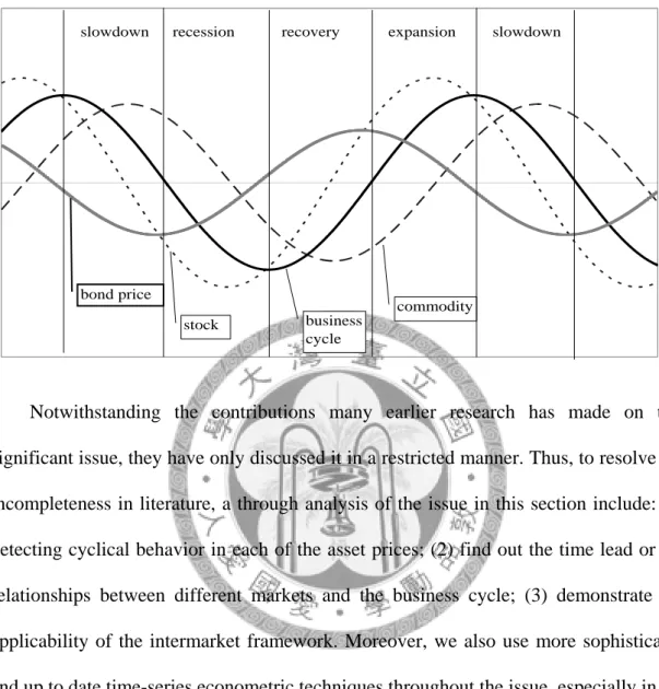
Intermarket analysis is the study of multiple asset classes in an integrated manner. Such an analytic framework has been widely used by finance practitioners and has been recognized as useful². The main reason why intermarket analysis can help investors enhance their profit is that peaks and troughs of a particular asset price cycle possesses a time lead or lag relationship corresponding to business cycle. In addition, the lead or lag relationships can be arranged orderly in a time sequence. Typically, in expansions, bond prices peak and then stock prices peak, followed by the peak of business cycle and then finally the peak of commodity prices, while also bottoming in the same order during contractions as well (Pring, 1992, 2002; Murphy, 2004)³. This stylized sequence is shown in Figure 1.1. By understanding this rotation chronology via intermarket analysis, an investor can have the bigger picture and would be able to see significant market and economic changes earlier than other investors only with a single market focus.

2

The Journal of Technical Analysis (Summer-Autumn 2002) had asked the membership of the Market Technicians to rate the relative importance of technical disciplines for an academic course on technical analysis. Of the fourteen disciplines included in the poll, intermarket analysis ranked fifth, while the cycle analysis ranked sixth (Charlton and Earl, 2006).

3

For example, the 10 years government bond prices and S&P 500 has reached its peak in March and September, 2007 that is nine and three months before the business cycle peak recognized by NBER.

Besides, the RJ/CRB commodity price index has reached its peak in June, 2008, which is six months after

Figure 1.1 An idealized diagram of how bond, stock and commodity interact during a typical business cycle

bond price

stock business

cycle

commodity

slowdown recession recovery expansion slowdown

Notwithstanding the contributions many earlier research has made on this significant issue, they have only discussed it in a restricted manner. Thus, to resolve the incompleteness in literature, a through analysis of the issue in this section include: (1) detecting cyclical behavior in each of the asset prices; (2) find out the time lead or lag relationships between different markets and the business cycle; (3) demonstrate the applicability of the intermarket framework. Moreover, we also use more sophisticated and up to date time-series econometric techniques throughout the issue, especially in the verification of cyclical relationships, with formal statistical testing.

The main purpose of the section is to apply the spectral analysis to detect cyclical behaviors in bond, stock and commodity markets and the business cycle and find out the lead or lag relationships among them. We will also demonstrate the applicability of the intermarket analysis based on the result of our spectral analysis.

2.2. A Review of Earlier Studies

A lot of literature has discussed the relationship between prices of various assets and the business cycle and also the applicability of such a framework. We first review the relationship between prices of different assets and the business cycle, and then we discuss the applicability of such framework in literature.

2.2.1. The Relationship between Different Asset Prices and the Business Cycle

Intermarket relationship between prices of different assets and the business cycle is not a new issue. In the influential book Turning Points in Business Cycles, Ayres (1939) raise the idea that intermarket analysis is an important way to better gauge the position of the economy relative to the business cycle:

…business cycles never repeat. Each one is an historical individual. … Because all business cycles are highly individualistic, and each is different from all the others, a typical cycle is of necessity a kind of mathematical abstraction….It is worth while to attempt to construct a typical cycle … It promotes understanding of the changing relationships that are always going forward between and among the major financial series that participate in the successive phases as the cycle expands from depression to prosperity, and then contracts from prosperity back down again to depression.

Therefore, he reviewed the five series that covered the histories of 24 complete

short term interest rates, bond prices, stock prices and security issues. He found that bond price and stock price peak before the business activity reach the peak.

Ayres’s work inspired many following researchers to find the typical sequence of the business cycle. The most eye catching follower was Geoffrey Moore (1975, 1990), once the chairman of National Bureau of Economic Research (NBER). In his book entitled Leading Indicators for the 1990s, Moore presented research supporting the chronological sequence between bonds and stocks as leading indicators of turns in the business cycle at peaks and troughs. He verified the lead or lag relationships between stock prices and the business cycle and also between bond prices and the business cycle by investigating simple accumulated returns on stocks and bonds, with the reference business cycle turning points recognized by NBER. What he found was that bonds turn first at peaks and troughs (with an average lead time of 17 months), and then stock (with an average lead time of 7 months). Moore’s research supports one of the basic premises of intermarket analysis, namely those bonds and stocks are not only linked, but peak and trough in a predictable rotational sequence. Following Moore’s method, Oppenlander (1997) also obtained the same conclusion.

Similar results were also obtained by Stock and Watson (1999) in their work

Business Cycles Fluctuations in US Macroeconomic Time Series which is a chapter in Handbook of Macroeconomics. They examines the empirical relationship in the post

war United States between the business cycle and various aspects of economic time series including bond prices and stock prices. This is done by calculating cross correlation between cyclical components of different economic time series. Note that the cyclical components are derived by BK filter.

Since commodity prices have become the issue in recent year, Pring (1992, 2002)

and Murphy (2004) have shown the intermarket relationships between bonds, stocks and commodities markets with the business cycle through graphic analysis, but they failed to include statistical analysis. They found that in expansions, bond prices peak and then stock prices peak, followed by the peak of business cycle and then finally the peak of commodity prices, while also bottoming in the same order during contractions as well.

2.2.2. The Applicability of Intermarket Framework

There was also a lot of research on the applicability of the intermarket framework, such as Pring (1992, 2002), Brocato and Steed (1998), Siegel (1991) and Gorton and Rouwenhorst (2006).

Even though he didn’t demonstrated the application of intermarket framework, Pring (1992, 2002) was the one of the earliest to illustrate how to allocate assets among bonds, stocks and commodities over the business cycle. Pring describes six stages of the business cycle and what happens to each asset class during each stage. Stage 1 (during recession) sees rising bond prices. Stage 2 is characterized by rising stocks. Stage 3 sees rising commodities. Stage 4 has bond prices peaking. Stage 5 shows stocks peaking.

Stage 6 is identified by falling commodities (during the onset of recession). He suggests a rotation where bonds turn first at peaks and troughs, stocks second and commodities last.

Brocato and Steed (1998) compared the performance of two portfolios. One is dynamic a portfolio which include bonds and stocks and would be cyclically relocated.

The other is a static portfolio which includes the same assets in a hypothetical

buy-and-hold strategy. They found that cyclically reallocating the portfolio consisted of equity and bond considering the business cycle can improve the return to risk ratio and make the portfolio more efficient.

As demonstrated by Siegel (1991), common stock returns can be significantly enhanced by a strategy that relies on correctly forecasting the turning points of the business cycle and reacting to it before the formal announcement of business cycle peaks and troughs by NBER.

Based on basic statistical analysis⁴, Gorton and Rouwenhorst (2006) had illustrated the negative correlation between commodity returns and equity and bond returns as probably due to the different price behavior of bond, equity and commodity assets throughout the business cycle. Therefore, inclusion of commodity assets as an option can enhance the efficiency of investment portfolios.

However, the discussions above were in restricted manner with only the stock market and the bond market (Brocato and Steed, 1998; Siegel 1991), some were also presented with only basic statistic operations (Gorton and Rouwenhorst 2006).

Therefore, in the next two sections, we should provide more rigorous evidence on this significant issue.

4

They use NBER business cycle dates to divide the business cycle into four phases－early expansion,

late expansion, early recession and late recession. Phases are identified by dividing the number of months

form peak to trough (trough to peak) into equal halves to indicate early recession and late recession (early

expansion and late expansion). Hence, they compare average returns of different assets over these four

business cycle phases.

2.3. Rationales and Empirical Verification of the Existence of Intermarket Relationships

2.3.1. Rationales of the intermarket relationships

In order to get a better handle on this concept, we will explain how and why these relationships exist and how the business cycle influences market activities. Among the different markets and the business cycle of our interest in this section, the business cycle is the focal point of the intermarket chain (Moore, 1990; Harvey, 1989; Stock and Watson, 1999). If we separate a complete business cycle into four phases－expansion, slowdown, recession and recovery phases just as Schumpeter (1939) did, we will find out lead or lag relationships of these three markets in relation to the business cycle are due to their different behaviors in each business cycle phase. As illustrated in Figure 1.1, the horizontal line is the potential growth path that separate positive output gap and negative output gap of economic activity. The curved line labeled business cycle shows the economy activity during alternating periods of expansion, slowdown, recession and recovery phases. When the curve line is above the horizontal line but increasing (decreasing), the economy is in its expansion (slowdown) phase. While the curve line is below the potential growth path but decreasing (increasing), the economy is in its recession (recovery) phase.

In the expansion phase, utilization rate of the economy is high, with booming investment activities and inflation pressure. In such circumstances, central banks would tighten their monetary policies and cause interest rates to rise, making bond markets bearish. In addition, commodity prices will rise at this phase due to strong demand induced by flourishing investment activities. Even stock markets would be bullish with

interest rates are likely to have an unfavorable effect on stock price (Moore, 1983; Pring, 1992, 2002; Murphy, 2004). The higher the yield on bonds, the more attractive they become as an alternative to holding stocks. Furthermore, higher interest rates and the accompanied reduce on availability of credit may diminish the propensity of investors to borrow money for buying stocks. Moreover, higher interest rates increase the cost of doing business, notably the cost of holding inventory, and hence may adversely affect profit margins even at a time the economy is still in its expansion phase (Moore, 1975).

In the slowdown phase, inflation remains high at beginning of this phase and utilization rate starts to deteriorate from its highest level. Profit margins of corporations shrink as economic growth slows down, making stock markets bearish. However, commodity markets may remain prosperous at the start of this stage despite economic activities are slowing down for two reasons. First, commodity demands are usually closely related to investment activities. Even when the economy has started to slowdown, since investments take time to build, it may prove difficult for involved parties to discontinue investment projects halfway, which will in order keep demand for commodities on a plateau. Second, commodity suppliers have time lags in their response to commodity price changes. Hence, despite the initiating economic downturn, suppliers have yet fully responded to the strong commodity demand, creating an elongated period of excess demand. Eventually, weaker economic performance finally form the peak of the commodity markets and the economy enters a low inflation environment in most cases, implying that interest rates may be falling, which will lead to bullish bond markets at the end of this stage,.

Regarding the recession phase, low inflation rates keeps interest rates low and makes the bond markets stay bullish. However, when nearing the end of this stage, the

fall in interest rates helps the market for stocks, and if the customary early upturn in profits also occurs, optimism among investors in common stocks is doubly justified even though business activity is still depressed and sliding downwards (Moore, 1983).

Notably, with the slack utilization rate of the economy, investment demand is low at this stage, keeping the commodity markets bearish.

As for the recovery phase, stock markets are still bullish due to improvement of profit and low interest rates. On the other hand, the low utilization rate keep firms reluctant to invest, which further keeps the commodity markets bearish at the beginning of this stage. Nevertheless, since economic recovery has took place for a period of time, forward looking central banks starts to initiate tightening monetary policies that directs interest rates to climb, which makes bond prices to reach its peak at the end of this stage.

In sum, the peaks (troughs) of the stock market usually occur at the end of expansion (end of recession phases), which all lead the turning points of the business cycle. The peaks (troughs) of the bond markets usually occur at the end of recovery (end of slowdown phases), which not only lead the turning points of the business cycle but also lead the corresponding turning points of the stock markets. However, the peaks (troughs) of the commodity markets usually come at the end of the slowdown (end of the recovery) phase, which not only lags behind the turning points of the business cycle but also the corresponding points of the other two markets.

2.3.2. Data

The data we use in this section includes the 10 year US Treasury bond prices, industrial production index (both downloaded from FRB St. Louis), S&P 500 stock price index (from the Bloomberg terminal), and the equally-weighted index of commodity futures (from NBER)⁵, covering data from May, 1960 thru December, 2007. In order to compare the performance of multiple assets, we transform the three market indexes into total return indexes.

To satisfy the stationary requirement of spectral analysis, our data is processed by the BK filter, so that the frequencies 18~180 months remain⁶. Furthermore, previous studies about the lead or lag relationships between asset prices and economic activity often use the accumulated return (or annual growth rate) of assets and reference business cycle dates to interpret their relationships. However, such comparison is statistically inappropriate, since reference dates of business cycles in practice is the date where absolute decline in the level of either the reference series or the detrended reference series initiate. However, the peak of growth rate in such reference series may have already been passed. Therefore, even if previous literature has verified the lead or lag relationships between asset prices and economic activity, the relationship may be an artifact. But we can avoid the aforementioned drawback by filtering the economic series

5

The total return index of the equally-weighted index of commodity is constructed by Gorton and Rouwenhorst (2008). It is available on the website at

http://www.nber.org/data-appendix/w10595/EqWtdTR_Jan_2008.xls.

6

Since the original series is only 52 years and 7 month in length and thus insufficient to discuss the

15-25 year Kuznets cycle and the 40-60 year Kondratieff cycle, all oscillations ranging from infinity to

15 years are treated as trends in this paper. Furthermore, fluctuations under 18 months are often regarded

as seasonal patterns or random noise. Consequently, the oscillations ranging from less than 15 to 1.5

years are defined as possible cyclical lengths of the cycles that we discuss in this section.

and asset prices with the same BK filter.

2.3.3. The existence of cyclical behavior

The characteristics of the cycles in each of the markets are first analyzed individually.

Our aim is to find out whether all these markets display the same propensity for cyclical fluctuations, and also whether they share the same regularity in those fluctuations. We apply the third test statistic proposed by Canova (1996) to test for the existence of cycles.

The results from spectral analysis show that the spectral density of S&P 500 is enlarged between two cyclical components, a shorter one at cycle length of 45 months, and another longer one with cycle length of 90 months. As for the 10 year Treasury bond, spectral density also magnify between two cyclical components, each with cycle lengths of 41.5 months and 90 months. Spectral densities of Commodity futures and industrial production, respectively, enlarge around the peaks in their spectrum density at 67.5 months (see Figure 1.2 and column 2 and 3 of Table 1.1). In other words, the four series seems to have similar cyclical behaviors, respectively.

Figure 1.2 Spectral density, S&P500, 10 years gov. bond, RJ/CRB, industrial production

0 0.05 0.1 0.15 0.2 0.25 0.3

0 0.01 0.02 0.03 0.04 0.05 0.06

S&P500 Spectrum Density

0 0.01 0.02 0.03 0.04 0.05 0.06 0.07 0.08 0.09

0 0.01 0.02 0.03 0.04 0.05 0.06

10Yr T-bond Spectrum Density

0 0.05 0.1 0.15 0.2 0.25 0.3 0.35 0.4 0.45

0 0.01 0.02 0.03 0.04 0.05 0.06

commodity Spectrum Density

0 0.005 0.01 0.015 0.02 0.025 0.03 0.035 0.04 0.045

0 0.01 0.02 0.03 0.04 0.05 0.06

industrial production Spectrum Density

Note: Shaded areas cover the frequencies

2 2

( , )

90 41

π π

Table 1.1 Univariate spectral statistic

Note: 1.Industrial production, S&P 500, 10 years government bond and commodity are named by IP, SP, Gov and Com respectively.

2. Sig. Freq and Sig. of Duration refers to frequency and corresponding duration of peak of spectrum.

3.

^*

,

^**

,

^***

denote the 90%, 95% and 99% of significant.

Whether the four series share the similar cyclical pattern in statistical sense is of

Peak Freq. Peak. Duration

(months) D

IP 0.0148 67.5 7.557

^***

SP 0.0111 & 0.0222 90 and 45 3.702

^***

Gov 0.0111 & 0.0241 90 and 41.5 3.208

^***

Com 0.0148 67.5 6.828

^***

interest and will be tested as follows. Define 2 2

( , )

90 41.5

π π

as Ω which is the union of ₁

frequencies with cycles, while 2 2 2 2

( , ) ( , )

180 90 41.5 18

π π π π

∪ is Ω . Applying the Canova ₂

test, the corresponding D statistics are shown on the column 4 of Table 1.1. To be sure, 2 2

( , )

90 41.5

π π

is significant at 99% confidence, which means the four markets

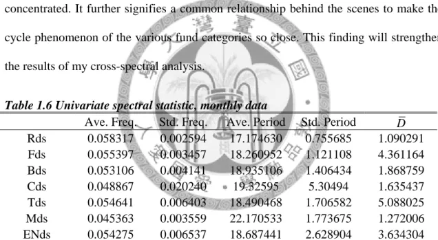
follow similar cyclical mechanisms in the span of 3.5 years to 7.5 years. In fact, the short cycle peaks of 41.5 months in the S&P 500 and 10 years Treasury bond, and 67.5 months in commodity futures and industrial production are interesting, since these frequencies are within the range of the well known 3~5 year Kitchin cycle (Kitchin, 1923). Besides, the long cycle peaks of 90 months in S&P 500 and Treasury bond all are within the frequencies of 7~11 year Juglar cycle (1862). Such results also provide evidence for the existence of Kitchin cycles and Juglar cycles in those markets.

In summary, we use Canova (1996)’s test to verify the existence of the cycles in various markets. It has especially shown that the frequency peaks of the power spectrum in these markets are rather coincident. It further hints that there are common relationships behind the scenes that link the seemingly independent markets altogether.

This finding will strengthen the results of our cross-spectral analysis.

2.3.4. Lead-lag relationship between markets

Before statistically verifying the lead or lag relationships between different markets, let’s take a look at the cyclical behavior in each of the markets. Figure 1.3 shows the filtered series of these markets with frequencies 2 2

( , )

90 41.5

π π

. The arrows of Figure 1.3

show quite clearly that the momentum of the bond prices leads the stock prices, the stock prices lead the industrial production, and the commodity futures lag behind all of them for most of the time.

Figure 1.3 Filtered series of 10-years gov. bond, S&P 500, industrial productions and commodity futures

Table 1.2 and Figure 1.4 is the summary of the cross-spectrum within the frequency of 2 2

( , )

90 41.5

π π

. Instead of SP/Gov and SP/Com failing to have significant

lead or lag relationship, the other four square coherences are all above the 0.349 mark, indicating significant lead or lag relationship in these four cases. Among them, industrial production has significant lead or lag relationships with the other three

Bond

-0.15 -0.1 -0.05 0 0.05 0.1 0.15

S&P 500

-0.20 -0.10 0.00 0.10 0.20 0.30

Industrial Production

-0.08 -0.06 -0.04 -0.02 0 0.02 0.04 0.06 0.08

Commodity

-0.25 -0.2 -0.15 -0.1 -0.05 0 0.05 0.1 0.15 0.2 0.25

1962 1964 1966 1968 1970 1972 1974 1976 1978 1980 1982 1984 1986 1988 1990 1992 1994 1996 1998 2000 2002 2004

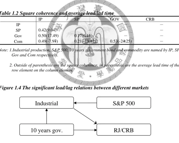
markets, in which it leads commodities for an average of 7.97 months and lags behind S&P 500 and treasury bonds for an average of 9.42 and 17.49 months, respectively.

This result indicates that economic fluctuation does influence financial markets. On the other hand, government bonds also lead commodities for 24.25 months. Noteworthy, the relationship between stock markets and economic activity and the relationship between bond markets and economic activity are similar to the results of Moore (1978), where he found that, on average, stock price peaks lead business cycle peaks for 5 months, while bond price peaks lead business cycle peaks for 14 months within the sample period 1943-73.

Table 1.2 Square coherence and average lead/lad time

IP SP GOV CRB

IP － － － －

SP 0.42(9.04) － － －

Gov 0.50(17.49) 0.17(6.15) － －

Com 0.49(-7.97) 0.21(-19.12) 0.53(-24.25) －

Note: 1.Industrial production, S&P 500, 10 years government bond and commodity are named by IP, SP, Gov and Com respectively.

2. Outside of parenthesis are the square coherence, in parenthesis are the average lead time of the row element on the column element

Figure 1.4 The significant lead/lag relations between different markets

Note: Arrows point to the lagging market

Nevertheless, although we cannot find significant lead or lag relationships between the S&P 500 index and government bond prices, and between the S&P 500 index and commodities, by indirect inferring the lag time of industrial production with S&P 500

Industrial

RJ/CRB S&P 500

10 years gov.

and with government bonds, we can find a weak support that bond prices lead the stock prices for roughly 8 months, which is similar to Moore’s (1975) results of 11 month lead. As for S&P 500 and commodities, even though the relationships are insignificant, we can also find a weak support that S&P 500 lead the commodities by indirectly inferring their individual lead or lag relationships with industrial production.

In summary, through the study of cross spectrum analysis, we verified that the commodities lag behind the other three markets, while the stock and bond markets, even tough their relationship with each other is ambiguous, both lead industrial production and commodities. Thus, our results give some evidence to Murphy (2004) and Pring’s (2002) idea that the order of lead or lag relationships among these four markets is bond market, equity market, economic activity and commodity market. Besides, the result can also reinforce the conclusion of Gorton and Rouwenhorst (2004).

2.5. Portfolio Return within Business Cycles

Are investors capable to increase their returns by implementing the aforementioned cyclical sequence among those markets? Actually, the implication of the cyclical sequence assumes investors can perfectly gauge their position in business cycles, where they should increase their stock positions before the economy reaches the trough, then switch to commodity assets before the economy reaches the peak, and then to bonds throughout most of the recession. If the investor can only choose between stocks and bonds, then the strategy is to increase stock positions before the trough and then reallocate to bonds nearing the peak. Noteworthy, the strategy with only stock and bond is similar to Siegel (1991), who has shown that portfolio returns can be enhanced significantly by switching between bonds and stocks before turning points in the

business cycle.

Table 1.3 is the summary results about whether commodity assets are a proper asset choice in the reallocation strategy based on the stages of business cycles. The first nine rows of Table 1.3 shows the summarized data of the US business cycle and the average annual return from investing in stocks, bonds and commodities over the business cycle. Over the entire period of May 1960 to December 2007, the seven recessions averaged 10.71 months in length, and expansions averaged 70.76 months in length, so that almost one-eighth of the time the economy in a recession.

Table 1.3 Average annual return of portfolio (May, 1960 － December, 2007)(bps)

(1) Average length of recession (months) 10.71

(2) Average Length of Expansion 70.67

(3) Average Length of Business cycle 81.38

(4) % of Time Economy in Recession 13.17

(5) % of Time Economy in Expansion 86.83

(6) Average Annual Return for Stock (%) 11.42 (7) Average Annual Return for Bonds (%) 7.59 (8) Benchmark Returns (6) X (5)+(7)X(4) (%) 10.92

(9) Average Annual Return for Com 12.36

(10) Average Returns of Portfolio (%)

Without Com With Com

0-month 1-month 2-month 3-month 4-month 5-month 6-month 6-month lead 14.01 15.35 15.71 16.16 15.64 15.19 15.47 15.67 5-month lead 13.85 14.93 15.47 15.93 15.26 14.82 14.96 15.02 4-month lead 14.31 14.66 15.21 15.45 14.78 14.38 14.53 14.59 3-month lead 14.22 14.34 14.89 15.13 14.37 13.97 13.91 13.97 2-month lead 14.69 14.60 15.15 15.39 14.63 14.14 14.08 13.99 1-month lead 13.54 14.05 14.59 14.83 14.08 13.59 13.52 13.43 concurrent 12.65 － 13.19 13.43 12.68 12.20 12.13 12.25

1-month lag 12.00 － － 12.23 11.49 11.02 10.95 11.06

2-month lag 11.29 － － － 10.55 10.08 10.02 10.13

3-month lag 10.88 － － － － 10.40 10.34 10.45

4-month lag 10.21 － － － － － 10.15 10.26

5-month lag 9.72 － － － － － － 9.84

6-month lag 9.82 － － － － － － －

From May 1960 thru December 2007, the average annual nominal return from

investing in the stock market is 11.42%, while the average return is 7.59% and 12.36%

from investing in 10-year Treasury bonds and the commodity index, respectively. The risk-adjusted return, the “benchmark” or “traditional asset class” return, is defined as the weighted average return with only stocks and bonds in the portfolio for the period and weighted according to the time the economy is in expansion (for stocks) and recession (for bonds), is 10.92%.

The column labeled “without Com” in the lower part of Table 1.3 is the return of reallocating only between stock and bond assets throughout the business cycle. The slot labeled “concurrent” reports returns from being 100% long in equities during economic expansion and 100% long in Treasury bonds during economic contractions. The returns calculated in “h-month lead” assumes an investor who leads the business cycle peaks for h-months in switching from stocks to bonds in business cycle expansions and leads the business cycle troughs also for h-months in switching from bonds to stocks in recessions. In contrast, an investor who lags the business cycle turning points to switch out of, and then into stocks an equal number of months after the peak and trough of the business cycle are labeled “h-month lag”. Actually, the results in the column labeled

“without Com” is similar to Siegel (1991), that investors can increase their returns by switching into bonds before the peak of the business cycle and into stocks before the trough of the business cycle.

The remaining part of Table 1.3 shows whether investors can increase returns by including commodity assets in their portfolio in some stages of the business cycle.

Noteworthy, as previous subsections have shown, bull commodity markets can go on even after the economy has passed its peak. Therefore, the investor can switch from stock assets to commodity assets before the peak of the business cycle and switch to