A Parallelized Learning Algorithm for Monotonicity Constrained Support Vector
Machines
Hui-Chi Chuang
Institute of Information Management National Cheng Kung University
Tainan City, Taiwan, R.O.C. e-mail: [email protected]
Chih-Chuan Chen
Interdisciplinary Program of Green and Information Technology
National Taitung University Taitung, Taiwan, R.O.C. e-mail: [email protected]
Chi Chou
Institute of Information Management National Cheng Kung University
Tainan City, Taiwan, R.O.C. e-mail: [email protected]
Yi-Chung Cheng
Department of International Business Management Tainan University of Technology
Tainan City, Taiwan, R.O.C. e-mail: [email protected]
Sheng-Tun Li
Institute of Information Management, Department of Industrial and Information Management
National Cheng Kung University Tainan City, Taiwan, R.O.C. e-mail: [email protected]
Abstract—Various efforts have been made to improve support vector machines (SVMs) based on different scenarios of real world problems. SVMs are the so-called benchmarking neural network technology motivated by the results of statistical learning theory [1], [2]. Among them, taking into account experts' knowledge has been confirmed to help SVMs deal with noisy data to obtain more useful results. For example, SVMs with monotonicity constraints and with the Tikhonov regularization method, also known as Regularized Monotonic SVM (RMC-SVM) incorporate inequality constraints into SVMs based on the monotonic property of real-world problems and the Tikhonov regularization method is further applied to ensure that the solution is unique and bounded. These kinds of SVMs are also referred to as knowledge-oriented SVMs. However, solving SVMs with monotonicity constraints will require even more computation than SVMs. In this research, a parallelized learning strategy is proposed to solve the regularized monotonicity constrained SVMs. Due to the characteristics of the parallelized learning method, the dataset can be divided into several parts for parallel computing at different times. This study proposes a RMC-SVMs with a parallel strategy to reduce the required training time and to increase the feasibility of using RMC-SVMs in real world applications.
Keywords-support vector machines; monotonic prior knowledge; learning algorithm; parallel strategy
I. INTRODUCTION
It is well-known that we are currently in the Big Data and Internet of Things (IOT) era. The progress in data processing and analyzing ability of computer hardware has fallen behind the growth of information such that the datasets are becoming too large to handle on a single hardware unit. In response, in this study we introduce an algorithm to deal with large-scale data by using a parallel strategy.
Many advanced data mining methods are being rapidly developed. Support Vector Machines (SVMs), were pioneered by Vapnik in 1995, and constitute a state-of-the-art artificial neural network (ANN) based on statistical learning [1], [2]. SVMs have been widely applied in many fields over the past few years, such as corporate distress, consumer loan evaluation, text categorization, handwritten digit recognition, speaker verification and many others.
Knowledge engineering is a process of developing an expert system that utilizes stored knowledge to achieve a higher performance, especially focusing on the knowledge provided by human experts in a specific field; in contrast, data mining focuses on data available in an organization. Recently, Li and Chen proposed a regularized monotonic SVM (RMC-SVM) for classification to a broader aspect of SVM by incorporating domain related intelligence in support vector learners for mining actionable knowledge for real-world applications [3], [4].
SVMs have high computing-time costs during the training procedure. The time complexity of SVMs is O (n2m) where m
represents the number of attributes and n represents the amount of data. So, if the data scale increases, SVM training becomes more complex and so requires more computational time. In addition, the SVMs model with regularized monotonic (RMC-SVM) causes change the structure of quadratic programming problem of SVMs and time complexity is more complicated. However, traditional training algorithms for SVMs, such as chunking and sequential minimal optimization (SMO) [5], [6], have computation complexity dependent on the amount of data, and become infeasible when dealing with large scale problems [7] and SVMs with monotonicity constraints. We chose the numerical analysis method with parallel strategy to solve the aforementioned problems.
The learning algorithm, proposed by Hestenes and Stiefel (1952), is an efficient numerical analysis method that converges quickly to find optimal solutions. With the characteristic of the parallelized learning algorithm, the dataset can be easily divided into P parts for parallel computing at different times or in separate computer hardware units. The parallelized learning algorithm is highly efficient in solving RMC- SVM and enhances the RMC-SVM algorithm making it more practical to use.
II. LITERATURE REVIEW
This section provides a review of the Support Vector Machines and the related literature to build the foundation of our study.
SVMs are the so-called benchmarking neural network technology motivated by the results of statistical learning theory [2], [8]. SVMs are primarily designed for binary classification, attempting to find out the optimal hyper-plane that separates the negative datasets from the positive datasets with maximum margin. They were originally developed for pattern recognition [9], and used a typically small subset of all training examples called the support vector to represent the decision boundary [10]. The optimal hyper-plane will accurately separate the data if the problem is linearly separable. However, since most of the datasets are non-separable, SVMs first map the same points onto a high-dimensional feature space to successfully separate non-separable data by the linear decision boundary in the input space. Moreover, SVMs use inner-product to overcome the high-dimensionality problems that machine learning methods are too difficult to solve [11].
For the purpose of improving the effectiveness or efficiency of SVMs, several theoretical studies have been conducted to modify or reformulate the conventional SVM model. Kramer et al. [12] presented a fast compression method to scale up SVMs to handle large datasets by applying a simple bit-reduction method to reduce the cardinality of the data by weighting representative examples. Also, Yu et al. [13] proposed two implementations of the block minimization framework for primal and dual SVMs, and then analyzed the framework for data which is larger than the memory size. At each step, a block of data is loaded from the disk and handled by certain learning methods. In recent years, the applications of SVM methods still exist over a wide range of fields.
Monotonicity is considered as a common form of prior knowledge and it can be constructed by lots of properties. Practically, people hope that the predictor variable and responding variable can satisfy the monotonicity property in problems. Pazzani et al. [14] addressed the importance of using monotonicity constraints in classification problems. Doumpos and Zopounidis [15] proposed a monotonic support vector machine. The virtual examples in this approach are generated from using the monotonicity “hints” to impose monotonic conditions, which represent prior knowledge associated with the problem. Finally, the model can reach a higher prediction accuracy and have a better prediction ability. Li and Chen [4] formulated a knowledge-oriented classification model by directly adding monotonicity constraints into the optimization model. To ensure the solution is unique and bounded, they applied Tikhonov regularization to alleviate the predicament caused by adding monotonicity constraints that might lead to
the loss of convexity [16], [17]. With the above study, we find that prior knowledge can increase the accuracy and bring up more valuable knowledge from data. We construct a SVM with monotonicity constraints and improve the result of the classification problem.
The learning method is one of the most useful techniques for solving large linear systems of equations, and it can also be adapted to solve nonlinear optimization problems. Besides, it is an iterative way to solve linear systems or nonlinear optimization problems and was introduced by Hestenes and Stiefel [18]. Thus, we can see that the parallelized learning method is very well suited for solving large problems.
The LS-SVM is an iterative training algorithm which is based on the parallelized learning method [19]. Moreover, the parallelized learning with SVMs is also used for intrusion detection [20]. Recently, Kaytez et al. [21] used LS-SVM to forecast the electricity consumption.
In many practical SVM applications, standard quadratic programming (QP) solvers based on the explicit storage of the Hessian matrix G may be very inefficient or even inapplicable due to excessive memory requirements. When facing large scale problems, exploiting the inherent parallelism of data mining algorithms provides a direct solution by using the large data retrieval and processing power of parallel architectures. On parallelization of SVM, several issues must be addressed to achieve good performance, such as limiting the overhead for kernel evaluations and choosing a suitable inner QP solver. Zanghirati and Zanni [22] obtained an efficient sub-problem solution by a gradient projection-type method, which exploits the simple structure of the constraints, exhibits good convergence rate and is well suited for a parallel implementation. Other parallel approaches to SVMs have been proposed, by splitting the training data into subsets and distributing them to processors [23], [24]. Zani et al. [25] implemented a parallel software for solving the quadratic programming arising in training SVMs for classification.
III. RESEARCH METHODOLOGY
Let N be the data number, and n be the number of attributes. A dataset 𝔍 = {(𝑥𝑖, 𝑦𝑖) | 𝑖 = 1,2, … , N }, with input data 𝑥𝑖∈ ℛ𝑛 and output data 𝑦
𝑖∈ ℛ. Then, the function ℱ(𝑥) ∶ ℛ𝑛→ ℛ is to stand for using input variables to classify the output variable. A partial ordering ≤ is defined over input space ℛ𝑛. A linear ordering ≤ is defined over the space ℛ with class labels as integer values 𝑦𝑖. The classified function is monotonic if it satisfies the following statement:
𝑥𝑖 ≤ 𝑥𝑗 ⇒ ℱ(𝑥𝑖) ≤ ℱ(𝑥𝑗), for any 𝑥𝑖 and 𝑥𝑗 (1) In this paper, we define the partial order on the input space ℛ𝑛 in an intuitive way such that for 𝑥 = (𝑥
1, 𝑥2, … , 𝑥𝑛) and 𝑥′= (𝑥
1′, 𝑥2′, … , 𝑥𝑛′), we say 𝑥 ≤ 𝑥′ if and only if 𝑥 ≤ 𝑥′ for 𝑖 = 1,2, … , n. For a classification problem, we say a target function has a monotonicity property if the experts perceive it as monotonic.
This study adopted a heuristic approach to enhance the monotonicity of an SVM classifier. To incorporate the monotonic prior knowledge into a problem, we denote a number of random pairs of virtual examples as
The predicted outcomes of the SVM classifier should satisfy the monotonicity constraints, ℱ(𝑥𝑖) ≤ ℱ(𝑥𝑗) for 𝑘 = 1, … , 𝑀, as closely as possible.
The idea of creating monotonicity constraints is straightforward since this kind of prior knowledge is provided by human experts from a specific field. Due to the expectation that the respective predicted classes 𝑦 and 𝑦′ satisfy the condition 𝑦 ≤ 𝑦′, constraints 𝒘𝑻𝝋(𝒙) ≤ 𝒘𝑻𝝋(𝒙′) can be added into a model for each pair of input vectors 𝒙 ≤ 𝒙′ to hold the monotonicity.
The primal SVM model is presented as min J(𝒘, 𝛆) = 1 2‖𝒘‖ 2+ 𝐶 ∑ 𝜀 𝑖 𝑁 𝑖=1 , 𝑠𝑢𝑏𝑗𝑒𝑐𝑡 𝑡𝑜 𝑦𝑖(𝒘𝑻𝝋(𝒙𝒊) + 𝑏) ≥ 1 − 𝜀𝑖, 𝑖 = 1, … , 𝑁, (2) 𝜀𝑖≥ 0, 𝑖 = 1, … , 𝑁
From the previous section, we know how monotonicity constraints can be constructed; and here, they are expressed as the following inequality:
𝒘𝑻𝝋(𝒙) ≤ 𝒘𝑻𝝋(𝒙), for observation 𝒙 ≤ 𝒙. (3)
By adding the monotonicity constraints to SVM, the model becomes as shown below and it is called MCSVM.
min J(𝒘, 𝛆) = 1 2‖𝒘‖ 2+ 𝐶 ∑ 𝜀 𝑖, 𝑁 𝑖=1 𝑠𝑢𝑏𝑗𝑒𝑐𝑡 𝑡𝑜 𝑦𝑖(𝒘𝑻𝝋(𝒙𝒊) + 𝑏) ≥ 1 − 𝜀𝑖, 𝑖 = 1, … , 𝑁, 𝒘𝑻𝝋(𝒙 𝑘) ≤ 𝒘𝑻𝝋(𝒙𝑘), for observations (4) 𝒙𝑘≤ 𝒙𝑘, 𝑘 = 1, … , 𝑀, 𝜀𝑖≥ 0, 𝑖 = 1, … , 𝑁.
Note that both the objective function and constraints are nonlinear in the above optimization problem. Since it is quite complicated to directly solve the problem in (5) with the possibility of 𝝋(𝒙) and 𝒘 being infinite dimensional, this problem can be solved in the dual space of a Lagrangian multiplier. When the kernel does not satisfy Mercer’s condition, it is possible that the matrix G is indefinite depending on the training data, and in this case the quadratic programming is non-convex and may have no solution [11]. Accordingly, the well-known Tikhonov regularization approach is applied to avoid this situation [16], [17]. A penalty term, δ which is set to be two times the absolute value of the minimal negative eigenvalue of matrix G is added to the objective function, after which the regularized model becomes
min 𝜶,𝜷 𝑄̃(𝜶, 𝜷) = 1 2[𝜶 𝑇 𝜷𝑇](G + 𝛿𝚰) [𝜶 𝜷] − 1𝑇𝜶, 𝑆𝑢𝑏𝑗𝑒𝑐𝑡 𝑡𝑜 ∑ 𝛼𝑖𝑦𝑖= 0, 𝑁 𝑖=1 0 ≤ 𝛼𝑖≤ 𝐶, 𝑖 = 1, … , 𝑁, (5) 𝛽𝑘≥ 0, ∀𝑘 = 1, … , 𝑀.
where 𝚰 is the identity matrix. With an appropriate choice of 𝛿, the quadratic programming problem would be convex and have a global solution. The resulting model is called a Regularized Monotonic SVM (RMC-SVM) model.
Finally, with an appropriate choice of kernel 𝐾 , the nonlinear RMC-SVM classifier takes the form:
𝑦(𝒙) = 𝑠𝑖𝑔𝑛 [∑𝑖=1𝑁 𝛼𝑖𝑦𝑖𝐾(𝑥𝑖, 𝒙) + ∑𝑀𝑘=1𝛽𝑘(𝐾(𝑥𝑘, 𝒙) − 𝐾(𝑥𝑘, 𝒙)) + 𝑏] (6)
where the 𝛫(𝒙𝒊, 𝒙𝒋) = 𝝋(𝒙𝒊)𝑇𝝋(𝒙𝒋)
The solutions, 𝛼𝑖′𝑠 and 𝛽𝑘′𝑠, are derived from the quadratic programming problem in (6).
The parallelized learning method, introduced by Hestenes and Stiefel [18], is an iterative method and one of the most useful techniques for solving large linear systems of equations; additionally, it can also be adapted to solve nonlinear optimization problems. The Parallelized learning method proceeds by generating vector sequences of iterates, residuals corresponding to iterates, and search directions used in updating iterates and residuals. In every iteration of the method, two inner products are performed in order to compute update scalars that are defined to ensure the vector sequences satisfy certain orthogonality conditions. On a symmetric positive definite linear system, these conditions imply that the distance to the true solution is minimized in some norm.
We take the parallelized learning method to solve the RMC-SVM model which is one of the numerical analysis methods used in this paper. The original RMC-SVM model is a quadratic programming problem with the constraints, including the equality constraint and the box constraint.
The box constraint restricts the range of estimate solutions, which has upper and lower bounds. Due to the parallelized learning method being used to solve unconstrained optimization problems, we modified it. We used the Lagrangian multiplier to transform the equality constraint into an objective function. Furthermore, we restrict the upper and the lower bounds of the estimate solution to deal with the box constraint in each iteration. We use the Lagrangian multiplier to transform equality constraint into an objective function. ℒ̃(𝜶, 𝜷, 𝝀) = 1 2[𝜶 𝑇 𝜷𝑇](G + 𝛿𝚰) [𝜶 𝜷] − 𝑒𝑇𝜶 + 𝛌𝑻(𝜶𝑦) = 12[𝜶𝑇 𝜷𝑇](G + 𝛿𝚰) [𝜶 𝜷] − (𝑒𝑇− 𝛌𝑻𝑦) 𝜶 (7) The details of parallelized learning method to solve the
RMC-SVM are shown in Figure 1.
Figure 1. Process of parallelized learning method to solve the RMC-SVM
Due to the structure of the SVM model with monotonicity constraints, the model becomes increasingly complicated. As such, we take the parallel strategy to solve the complex RMC-SVM model. It is similar to the Divide-and-Conquer algorithm. First, the dataset is averagely divided into m parts, which is called divide. Second, each part of the dataset is individually
Let the objective function 𝐹(𝑥) = 1 2 𝑥
𝑇𝑄𝑥 − 𝑒𝑇𝑥 where x is an n by n matrix with the equality constraint 𝐺(𝑥) = 𝑦𝑥 Initiate vector, including the number of executions, the estimate solution, and search direction
Repeat
1. Compute the scalar 𝛼 and update the next estimate solution
2. Compute the Lagrangian multiplier 𝜆 and ∇𝐿(𝑥)=∇𝐹(𝑥) + λ ∇𝐺(𝑥)
3. Update the search direction 𝑑(𝑘+1)= ∇𝐿(𝑥) + 𝑟𝑘𝑑(𝑘) where 𝑟𝑘= ∇L(𝑥𝑘+1)∗ ∇L(𝑥𝑘+1)
𝑇
∇L(𝑥𝑘)∗∇L(𝑥𝑘)𝑇
operated, which is called conquer. Finally, the mixture algorithm is used to integrate the results of different parts. To parallelize RMC-SVM, we first split the dataset and apply the parallelized learning algorithm proposed in the previous subsection. For data splitting, the parallel mixture of SVMs for large scale problems [23] is adopted for solving RMC-SVM. The idea is to divide the training set into m random subsets of approximately equal size. Each subset, called an expert, is then trained separately and the optimal solutions of all sub- SVMs are combined into a weighted sum, called "gater" module, to create a mixture of SVMs.
Finally, another optimization process is applied to determine the optimal mixture. The idea of mixtures has given rise to very popular SVM training algorithms.
The output of the mixture is defined as follow
𝑓(𝑥) = [ℎ ∑𝑃𝑗=1𝜔𝑗(𝑥)𝑆𝑗(𝑥)] (8)
where h is a transfer function which could be, for instance, the hyperbolic tangent for classification tasks. ωi (x) is the gater weight, and is trained to minimize the cost function:
𝜔 = ∑𝑁𝑖=1[𝑓(𝑥𝑖) − 𝑦𝑖 ] (9)
𝑆𝑖(𝑥) is the output of each expert, and the output in RMC-SVM is as follows:
𝑆𝑖(𝑥) = ∑𝑖=1𝑁 𝛼𝑖𝑦𝑖𝐾(𝑥𝑖, 𝒙) + ∑𝑀𝑘=1𝛽𝑘(𝐾(𝑥𝑘, 𝒙) − 𝐾(𝑥𝑘, 𝒙)) + 𝑏 (10)
IV. EXPERIMENTAL RESULTS AND ANALYSIS
We evaluate the performance of the proposed parallel strategy algorithm to solve the RMC-SVM problem and discuss comparisons of the prediction results obtained by RMC-SVM, Mixture SVM and Mixture RMC-SVM on three real-world datasets.
Due to the dataset being too large for us to handle at one time, in this research we propose a more efficient algorithm that can accelerate the training time. In the experiment, we used three real-world datasets as presented in next subsection, the codes of which are executed in MATLAB R2015a on an Intel Core i7-4770 CPU 3.2 GHz with 16 GB RAM running Window Server 2008. Additionally, we use the same RBF kernel function with different methods.
In the experiment, we have nine steps, for which the details are listed as follows.
Step1. Preprocess the data and normalize each data element in the dataset.
Step2. Randomly partition the dataset into a two-one-split training set and a testing set.
Step3. In the same partitioned dataset, respectively train the data with RMC-SVM Mixture SVM and Mixture RMC-SVM.
Step4. In the Mixture RMC-SVM, divide the training set into
m parts, and each part respectively constructs
monotonic constraints.
Step5. For each part use grid search to find the optimal parameters C and σ.
C = {0.01 0.05 0.1 0.5 1 5 10 50 100 500 1000}, σ = {0.5 5 10 15 25 50 100 250 500}.
Step6. Use the output of each part to calculate the gater weight.
Step7. Compute the parameter mixture to integrate the output from each part and classify the data of the testing data.
Step8. Repeat step2 to step7 for 30 times.
Step9. Analyze the average performance result of the 30 times.
Our research conducted the experiments with one real-world dataset from the UCI [26] machine learning repository: Wisconsin Diagnostic Breast Cancer (WDBC). The WDBC dataset is computed from digitized images of fine needle-aspirated (FNA) breast mass, in which characteristics of the cell nuclei present in the images are described. For the WDBC dataset, there were 683 instances after removing missing values. Furthermore, each instance consists of nine attributes and distinguishes the class label for whether the cell is malignant or benign.
In this research, we compare our proposed parallel strategy algorithm with MCSVM. The performance results are examined in terms of Accuracy, F-measure, frequency monotonicity rate (FMR) and training time.
Accuracy is the most intuitive measurement criterion, which directly defines the predictive ability based on the proportion of the tested data that are correctly classified, and is defined as follows:
𝐴𝑐𝑐𝑢𝑟𝑎𝑐𝑦 = 𝑇𝑃 + 𝑇𝑁
𝑇𝑃 + 𝐹𝑃 + 𝑇𝑁 + 𝐹𝑁 (11)
Recall, also called Sensitivity, measures the proportion of actual positives that are correctly identified as such, and is defined as follows:
𝑅𝑒𝑐𝑎𝑙𝑙 = 𝑇𝑃
𝑇𝑃 + 𝐹𝑁 (12)
The precision rate, also named Positive Predictive Value (PPV), is the proportion of test instances with positive predictive outcomes that are correctly predicted. It is the most important measure of a predictive method, as it reflects the probability that a positive test reflects the underlying condition being tested for. It is defined as:
𝑃𝑟𝑒𝑐𝑖𝑠𝑖𝑜𝑛 = 𝑇𝑃
𝑇𝑃 + 𝐹𝑃 (13)
The traditional F-measure is the harmonic mean of recall (Sensitivity) and precision (PPV), and is defined as:
𝐹 − 𝑚𝑒𝑎𝑠𝑢𝑟𝑒 = 2 ∙ 𝑃𝑃𝑉 ∙ 𝑆𝑒𝑛𝑠𝑖𝑡𝑖𝑣𝑖𝑡𝑦
𝑃𝑃𝑉 + 𝑆𝑒𝑛𝑠𝑖𝑡𝑖𝑣𝑖𝑡𝑦 (14) The F-measure takes both recall and precision into account, thereby avoiding a situation with low recall and high precision, or vice versa.
We use the Frequency Monotonicity Rate (FMR) to measure the monotonicity of the dataset ℑ = {(x𝑖, 𝑦𝑖)|𝑖 = 1,2, … , 𝑁}, which is defined as the proportion of data pairs in a dataset that do not violate the monotonicity condition. It is defined as:
𝐹𝑀𝑅 =𝐹𝑀
𝑃 =
Number((𝑥𝑖≥ 𝑥𝑗) ∧ (𝑦𝑖≥ 𝑦𝑗))
C2𝑁 (15)
where 𝑃 is the number of observed pairs, and 𝐹𝑀 is the number of pairs that do not violate the monotonicity condition. Note that the monotonicity measure FMR can also be applied to a classifier in order to measure its capability of retaining monotonicity in an unseen dataset.
In the experiment, we conducted each process in the same training dataset. Both RMC-SVM and Mixture RMC-SVM used the hierarchy method to construct monotonicity constraints. It should be noted that the experiments carried out in this research have the following two different numbers of constraints:
number of constraints={63,127}
In this paper, we use the parallel strategy to solve the quadratic programming problem of RMC-SVM. We have two diverse directions to construct monotonicity constraints. We can use the whole training dataset or the dataset that divides the whole training dataset into different parts to construct monotonicity constraints. In the parallel strategy, the dataset is divided into different parts. Thus, the experiments selected three different numbers of parts to divide the whole dataset:
number of parts={2,4,6}
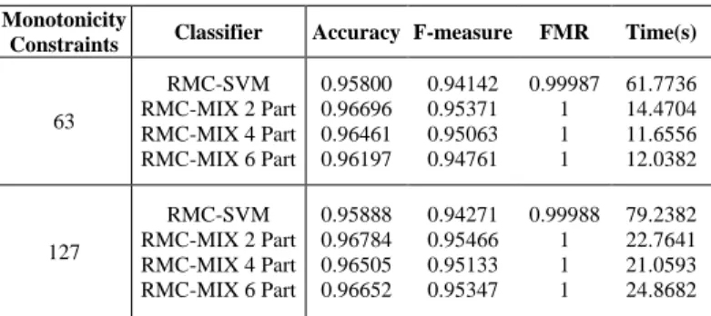
TABLEI. WDBC DATASET RESULTS Monotonicity
Constraints Classifier Accuracy F-measure FMR Time(s)
63 RMC-SVM RMC-MIX 2 Part RMC-MIX 4 Part RMC-MIX 6 Part 0.95800 0.96696 0.96461 0.96197 0.94142 0.95371 0.95063 0.94761 0.99987 1 1 1 61.7736 14.4704 11.6556 12.0382 127 RMC-SVM RMC-MIX 2 Part RMC-MIX 4 Part RMC-MIX 6 Part 0.95888 0.96784 0.96505 0.96652 0.94271 0.95466 0.95133 0.95347 0.99988 1 1 1 79.2382 22.7641 21.0593 24.8682
V. CONCLUSIONS AND SUGGESTIONS
In this paper, parallel strategy was used to solve SVMs with monotonicity constraints (RMC-SVM) in which the whole training dataset was partitioned into smaller subsets and then RMC-SVM was parallelly applied to each of the partitioned subsets. Furthermore, a mixture method was used to integrate the results from all subsets and to classify the testing dataset. Our experiment on two real world datasets demonstrated the efficiency of the parallel strategy RMC-SVM.
We explored the efficiency of the predictive performance of the parallel strategy to solve RMC-SVM with different numbers of parts to divide the whole training dataset in, as well as diverse directions to construct the monotonicity constraints. The experiment showed that the efficiency of the parallel strategy RMC-SVM decreases as the number of parts increases. It is because there is more communication and integration time with the use of more parts. Moreover, most of the experimental results showed that the proposed method had a better performance if the whole training dataset was used to construct monotonicity constraints as compared with using the subsets to construct monotonicity constraints. In the further, we will implement more experiments to verify our method.
ACKNOWLEDGMENT
This research was supported in part by the Ministry of Science and Technology, ROC, under contract MOST 105-2410-H-006-038-MY3. The authors also thank Mr. Chi Chou for his help on the experimentation.
REFERENCES
[1] Vapnik, “The Nature of Statistical Learning Theory,” 1995. [2] V. Vapnik, “Statistical learning theory,” Wiley: New York,Vol.
1, 1998.
[3] C. C. Chen, and S. T. Li, “Credit rating with a monotonicity-constrained support vector machine model. Expert Systems with Applications,” Vol. 41(16), 7235-7247, 2014.
[4] S. T. Li, and C. C. Chen, “A regularized monotonic fuzzy support vector machine model for data mining with prior knowledge,” IEEE Transactions on Fuzzy Systems, vol. 23(5), 1713-1727, 2015.
[5] C. C. Chang, and C. J. Lin, “LIBSVM: a library for support vector machines,” ACM Transactions on Intelligent Systems and Technology (TIST), vol. 2(3), 27, 2011.
[6] C. J. Platt, “12 fast training of support vector machines using sequential minimal optimization,” Advances in kernel methods, 185-208, 1999.
[7] A. K. Menon, “Large-scale support vector machines: algorithms and theory,” Research Exam, University of California, San Diego, 1-17, 2009.
[8] C. Cortes, and V. Vapnik, “Support-vector networks,” Machine learning, vol. 20(3), 273-297, 1995.
[9] B. E. Boser, I. M. Guyon, and V. N. Vapnik, “A training algorithm for optimal margin classifiers,” Paper presented at the Proceedings of the fifth annual workshop on Computational learning theory, 1992.
[10] B. SchiilkopP, C. Burgest, and V. Vapnik, “Extracting support data for a given task.” no. x, 1995.
[11] C. J. Burges, “A tutorial on support vector machines for pattern recognition,” Data mining and knowledge discovery, vol. 2(2), 121-167, 1998.
[12] K. Kramer, L. O. Hall, D. B. Goldgof, A. Remsen, and T. Luo, “Fast support vector machines for continuous data,” Systems, Man, and Cybernetics, Part B: Cybernetics, IEEE Transactions on, vol. 39(4), 989-1001, 2009.
[13] H. F. Yu, C. J. Hsieh, K. W. Chang, and C. J. Lin, “Large linear classification when data cannot fit in memory,” ACM Transactions on Knowledge Discovery from Data (TKDD), vol. 5(4), 23, 2012.
[14] M. J. Pazzani, S. Mani, and W. R. Shankle, “Acceptance of rules generated by machine learning among medical experts,” Methods of information in medicine, vol. 40(5), 380-385, 2001. [15] M. Doumpos, and C. Zopounidis, “Monotonic support vector
machines for credit risk rating,” New Mathematics and Natural Computation, vol. 5(3), 557-570, 2009.
[16] C. M. Maes, “A regularized active-set method for sparse convex quadratic programming,” Citeseer, 2010.
[17] A. N. Tikhonov, and V. I. A. k. Arsenin, “Solutions of ill-posed problems: Vh Winston,” 1977.
[18] M. R. Hestenes, and E. Stiefel, “Methods of learnings for solving linear systems,” 1952.
[19] J. Suykens, L. Lukas, P. Van Dooren, B. De Moor, and J. Vandewalle, “Least squares support vector machine classifiers: a large scale algorithm,” Paper presented at the European Conference on Circuit Theory and Design, ECCTD, 1999. [20] S. Mukkamala, G. Janoski, and A. Sung, “Intrusion detection
using neural networks and support vector machines,” Paper presented at the Neural Networks, 2002. IJCNN'02. Proceedings of the 2002 International Joint Conference on, 2002.
[21] F. Kaytez, M. C. Taplamacioglu, E. Cam, and F. Hardalac, “Forecasting electricity consumption: a comparison of regression analysis, neural networks and least squares support vector machines,” International Journal of Electrical Power and Energy Systems, vol. 67, 431-438, 2015.
[22] G. Zanghirati, and L. Zanni, “A parallel solver for large quadratic programs in training support vector machines,” Parallel computing, vol. 29(4), 535-551, 2003.
[23] R. Collobert, S. Bengio, and Y. Bengio, “A parallel mixture of SVMs for very large scale problems,” Neural computation, vol. 14(5), 1105-1114, 2002.
[24] J. x. Dong, A. Krzyżak, and C. Y. Suen, “A fast parallel optimization for training support vector machine Machine Learning and Data Mining in Pattern Recognition,” Springer, 96-105, 2003.
[25] L. Zanni, T. Serafini, and G. Zanghirati, “Parallel software for training large scale support vector machines on multiprocessor systems,” The Journal of Machine Learning Research, vol. 7, 1467-1492, 2006.
[26] C. L. Blake and C.J. Merz, UCI repository of machine learning databases. from http://www.ics.uci.edu/~mlearn/MLRepository. html, 1998, [accessed June 2017].