Stability analysis of neural networks with interval time-varying delays
Yi-You Hou and Teh-Lu Liaoa兲
Department of Engineering Science, National Cheng Kung University, Tainan 701, Taiwan
Chang-Hua Lien
Department of Marine Engineering, National Kaohsiung Marine University, Kaohsiung 811, Taiwan
Jun-Juh Yan
Department of Computer and Communication, Shu-Te University, Kaohsiung 824, Taiwan
共Received 18 October 2006; accepted 23 July 2007; published online 21 September 2007兲 The global exponential stability is investigated for neural networks with interval time-varying delays. Based on the Leibniz-Newton formula and linear matrix inequality technique, delay-dependent stability criteria are proposed to guarantee the exponential stability of neural networks with interval time-varying delays. Some numerical examples and comparisons are provided to show that the proposed results significantly improve the allowable upper and lower bounds of delays over some existing ones in the literature. © 2007 American Institute of Physics.
关DOI:10.1063/1.2771082兴
The stability analysis of a class of neural networks, such as Hopfield neural networks, cellular neural networks, and Cohen-Grossberg neural networks, has been exten-sively investigated; these particular networks have been applied to image processing and signal processing prob-lems. However, in this class of neural networks, the inter-actions between neurons are generally asynchronous, which inevitably results in time delay. The existence of time delay may cause oscillations and instability in neural networks. Therefore, the stability analysis of neural net-works with time delay is an important issue. The criteria for time-delay systems can be classified into two catego-ries; namely, independent criteria and delay-dependent criteria. Generally speaking, the latter group is less conservative than its counterpart when the time-delay values are small. In both of these analysis problems, the time delay is known to reside within an interval in-cluding zero, and the upper bound of the time derivative of time-varying delay is known and smaller than 1. In this paper, we propose a less conservative delay-dependent stability formula to guarantee the global expo-nential stability of neural networks with interval delays, which may exclude zero. Furthermore, the supplemen-tary requirement that the time derivative of time-varying delays must be smaller than one is not necessary in this study.
I. INTRODUCTION
Neural networks have great potential in practical appli-cations, such as static image processing, signal processing, etc. However, in the neural networks, the interactions be-tween neurons are generally asynchronous, which inevitably results in time-varying delays. Furthermore, time delay is frequently a source of instability and deterioration of a sys-tem’s performance; therefore, the stability analysis of
time-delayed systems has received considerable attention over the past several years. Recently, dynamical properties of delayed neural networks 共DNNs兲 have proven to be important in practical applications, such as image shadowing, system identification, and pattern recognition.1–5 Consequently, the stability analysis of DNNs has emerged as a new and attrac-tive research field in neural networks, such as delayed cellu-lar neural networks 共DCNNs兲, delayed Hopfield neural net-works 共DHNNs兲, and delayed Cohen-Grossberg neural networks 共DCGNNs兲. Many profound theories and method-ologies have been developed to deal with this issue.6–18The globally exponential stability,6,7 the existence of periodic solutions10–13of DCNNs and DCGNNs have been presented and the dynamic behaviors of DHNNs have been extensively investigated in Refs.14–18. In Refs.19and20, some suffi-cient conditions for global stability of DCGNNs have been provided, yet only constant delays are allowed in their re-sults. Hence, the stability of neural networks with time-varying delays has become more interesting than that of ones with constant time delays.21–32 However, the constraint ˙共t兲⬍1 on time-varying delay was imposed in Refs. 21–32. Such a restriction is very conservative and has physical limitations.
On the other hand, interval time-varying delays 0ⱕm
ⱕj共t兲ⱕMare used to indicate that the propagated speed of
signals is finite and uncertain in systems, such as network control systems.33 Under the interval time-delay condition, the robust H⬁control design for linear systems was studied in Ref.34, the delay-dependent robust stability for uncertain linear systems was proposed in Ref. 35, and the stability analysis and control synthesis of uncertain systems via Takagi-Sugeno fuzzy modes were presented in Ref. 36. Therefore, this paper contributes to the development of glo-bally exponential stability criteria for the neural networks with interval time-varying delays. The obtained results are derived based on the Lyapunov theory, the linear matrix in-equality 共LMI兲 technique, and the Leibniz-Newton formula.
a兲Electronic mail: tlliao@mail.ncku.edu.tw
共2007兲
Furthermore, the requirement˙共t兲⬍1 is not necessary in the proposed scheme. Finally, two illustrative examples are pro-vided to verify that our results are less conservative than that reported in the literature.21,22,24,25
Notation. Note that throughout the remainder of this pa-per, the notation Rn denotes the n-dimensional real space,
Rm⫻n is the set of all real m⫻n matrices, I is the identity matrix of appropriate dimension, C共关−M, 0兴,Rn兲 denotes the
set of all differentiable vector functions from关−M, 0兴 to Rn,
ATdenotes the transpose of matrix A,储x储 represents the
Eu-clidean norm of vector x, AⱕB means that B−A is a positive semi-definite matrix, P = PT⬎0 denotes that P is a
symmet-ric positive definite matrix, P = PT⬍0 denotes that P is a
symmetric negative definite matrix, min共P兲 denotes the minimal eigenvalue of the matrix P, andmax共P兲 denotes the maximal eigenvalue of the matrix P. The notation “*” in symmetric block matrices or long matrix expressions throughout the paper represents an ellipsis for terms that are induced by symmetry, e.g.,
冋
A B * C册
=冋
A B
BT C
册
.II. PROBLEM FORMULATION AND MAIN RESULTS
The dynamics of the neural networks with interval time-varying delays are described by the following differential equation: x˙i共t兲 = − cixi共t兲 +
兺
j=1 n aijfj关xj共t兲兴 +兺
j=1 n bijfj兵xj关t −j共t兲兴其 + Ji, tⱖ 0, i = 1, ... ,n. 共1兲System共1兲 can be rewritten in the following form:
x˙共t兲 = − Cx共t兲 + Af关x共t兲兴 + Bf兵x关t −共t兲兴兲 + J, t ⱖ 0 共2兲 where x共t兲=关x1共t兲¯xn共t兲兴T苸Rn and x关t−共t兲兴=兵x1关t
−1共t兲兴¯xn关t−n共t兲兴其T苸Rn, C = diag兵c1, c2, . . . , cn其 is a
positive diagonal matrix, while A =关aij兴n⫻n and B =关bij兴n⫻n
are known constant matrices, A is referred to as the feedback matrix, B represents the delayed feedback matrix with the time-varying delayj共t兲 and J is the external bias vector. In 共1兲 and 共2兲, it is assumed that 0ⱕmⱕj共t兲ⱕM and˙j共t兲
ⱕD, for all 1ⱕ jⱕn and tⱖ0. The initial condition of共2兲is
given by x共t兲=共t兲苸C共关−M, 0兴,Rn兲. f关x共t兲兴
=兵f1关x1共t兲兴, f2关x2共t兲兴, ... , fn关xn共t兲兴其T denotes the activation
function vector of the neurons whose components are con-tinuous with respect to x. Regarding the function fi, we make
the following assumption:
Assumption 1. Each function fi: R→R, i
苸兵1,2, ... ,n其 is monotonically nondecreasing, bounded, and satisfies the Lipschitz condition with a Lipschitz constant Li⬎0, i.e., 兩fi共u兲− fi共v兲兩 ⱕLi兩u−v兩 for all u,v苸R.
Remark 1. Several neural networks satisfy Assumption 1; in fact, if fi共x兲=tanh共xi兲, then共2兲 represents the Hopfield
neural networks with time-varying delays. Furthermore, if fi共x兲=共兩xi+ 1兩−兩xi− 1兩兲/2, then共2兲describes the cellular
neu-ral networks with time-varying delays.
Assume that an equilibrium point of 共2兲 exists and is given as x*=关x 1 *, x 2 *, . . . , x n *兴T.29–32
The aim of the paper is to propose some sufficient conditions to ensure the globally ex-ponential stability with a convergence rate␣for the equilib-rium point x*of system共2兲. Therefore, we make the
follow-ing definition.
Definition 1 (global exponential stability). The equilib-rium point x* of system (2) is said to be globally
exponen-tially stable with a convergence rate␣if constants␣⬎0 and ⱖ1 exist such that
储x共t兲 − x*储 ⱕ·
共
sup −Mⱕⱕ0 储x共兲 − x*储 + sup −Mⱕⱕ0 储x˙共兲储兲
e−␣t for all tⱖ 0. Shifting the equilibrium point to the origin and defining z共t兲=x共t兲−x*, where z =关z1, z2, . . . , zn兴T, then共2兲can be
trans-formed into the following form:
z˙共t兲 = − Cz共t兲 + A关z共t兲兴 + B兵z关t −共t兲兴其, ∀ t ⱖ 0, 共3a兲 z共t兲 =共t兲, t 苸 关−M,0兴 共3b兲 where关z共t兲兴=关兵1关z1共t兲兴,2关z2共t兲兴, ... ,n关zn共t兲兴其T, 兵z关t −共t兲兴其 =关1兵z1关t −1共t兲兴其,2兵z2关t −2共t兲兴其, ... , n兵zn关t −n共t兲兴其兴T, i关zi共t兲兴 = fi关zi共t兲 + xi *兴 − f i共xi *兲, i兵zi关t −i共t兲兴其 = fi兵zi关t −i共t兲兴 + xi *其 − f i共xi *兲.
Note that the function f共·兲 satisfies Assumption 1, and we have T关z共t兲兴关z共t兲兴 = 储关z共t兲兴储2ⱕ zT共t兲⌺2z共t兲 共4a兲 and T兵z关t −共t兲兴其兵z关t −共t兲兴其 = 储兵z关t −共t兲兴其储2 ⱕ zT关t −共t兲兴⌺2z关t −共t兲兴, 共4b兲 where⌺=diag兵L1, L2, . . . , Ln其.
Clearly, z = 0 is an equilibrium point of the system共3兲. If the origin of the system 共3兲is globally exponentially stable, then the equilibrium point x* of system共2兲 is also globally exponentially stable. Let zˆ共t兲=e␣tz共t兲; then system共3兲can be
transformed into the following form:
zˆ˙共t兲 = − 共C −␣I兲zˆ共t兲 + A˜关zˆ共t兲兴 + B˜关zˆ关t −共t兲兴兴
= − C˜ zˆ共t兲 + A˜关zˆ共t兲兴 + B˜关zˆ关t −共t兲兴兴, ∀ t ⱖ 0, 共5a兲
zˆ共t兲 =ˆ共t兲, t 苸 关−M,0兴, 共5b兲
where C˜ =C−␣I, ˜关zˆ共t兲兴=e␣t关z共t兲兴, ˜兵zˆ关t−共t兲兴其 = e␣t兵z关t−共t兲兴其, and ˆ共t兲=e␣t共t兲, t苸关−M, 0兴. Since the
function共·兲 satisfies共4兲, we have
˜T兵zˆ关t −共t兲兴其˜兵zˆ关t −共t兲兴其 =储˜兵zˆ关t −共t兲兴其储2 =
兺
i=1 n e2␣t·i2兵zi关t −i共t兲兴其 =兺
i=1 n e2␣i共t兲e2␣关t−i共t兲兴· i 2兵z i关t −i共t兲兴其 =兺
i=1 n e2␣i共t兲·˜ i 2兵zˆ i关t −i共t兲兴其 ⱕ兺
i=1 n e2␣i共t兲zˆ i T关t − i共t兲兴Li 2 zˆi关t −i共t兲兴 ⱕ e2␣MzˆT关t −共t兲兴⌺2zˆ关t −共t兲兴, 共6b兲 where⌺=diag兵L1, L2, . . . , Ln其.Before presenting the main results, let us introduce the following lemma:
Lemma 1. For a n⫻n symmetric positive definite matrix M, 0ⱕmⱕ共t兲ⱕM, tⱖ0, and any differentiable vector
function x共t兲苸Rn, we have 共a兲
冉
冕
t−m t x˙共s兲ds冊
T M冉
冕
t−m t x˙共s兲ds冊
ⱕm·冕
t−m t x˙T共s兲Mx˙共s兲ds, t ⱖ 0, 共b兲冉
冕
t−共t兲 t−m x˙共s兲ds冊
T M冉
冕
t−共t兲 t−m x˙共s兲ds冊
ⱕ关共t兲 −m兴 ·冕
t−共t兲 t−m x˙T共s兲Mx˙共s兲ds ⱕ 共M−m兲 ·冕
t−M t−m x˙T共s兲Mx˙共s兲ds, t ⱖ 0.Proof. The second inequality of 共b兲 is a trivial result. Now the first inequality of共b兲 must be proven. For any scalar and vector共t兲苸Rn, we have
冕
t−共t兲 t−m 关x˙共s兲 −共t兲兴T M关x˙共s兲 −共t兲兴ds ⱖ 0, t ⱖ 0. This implies 2·关共t兲 − m兴T共t兲M共t兲 − 2·冕
t−共t兲 t−m x˙T共s兲dsM共t兲 +冕
t−共t兲 t−m x˙T共s兲Mx˙共s兲ds ⱖ 0, t ⱖ 0.Since the above inequality is satisfied for anyand tⱖ0, we can obtain the following condition:
冉
2冕
t−共t兲 t−m x˙T共s兲dsM共t兲冊
2 − 4关
关共t兲 −m兴T共t兲M共t兲兴
·冉
冕
t−共t兲 t−m x˙T共s兲Mx˙共s兲ds冊
ⱕ 0. Letting 共t兲=兰t−t−共t兲mx˙共s兲ds, then关
T共t兲M共t兲兴
2−关
关共t兲 − m兴T共t兲M共t兲兴
·冋
冕
t−共t兲 t−m x˙T共s兲Mx˙共s兲ds册
ⱕ 0.Surveying above inequality, it is clear that the first inequality of共b兲 is always true for both= 0 and⫽0. Thus, the proof of the first inequality of 共b兲 is completed, and via similar derivations, inequality 共a兲 is also satisfied. 䊐 In the second, a delay-dependent criterion for the glo-bally exponential stability of the system 共3兲 with the same time-varying delays, i.e.,i共t兲=ˆ共t兲, i=1,2, ... ,n, is given in
the following theorem.
Theorem 1. The equilibrium point x* of system (2)
as-sociated with Assumption 1 and mⱕi共t兲=ˆ共t兲ⱕM, ˆ˙共t兲
ⱕD, i = 1 , 2 , . . . , n is globally exponentially stable with
con-vergence rate ␣⬎0, if there are some symmetric positive definite matrices P, Q1, Q2, R1, R2, matrices F1, F2, F3, and
some positive constantsand, such that the following LMI condition holds: ⌽ =
冤
⌽11 ⌽12 ⌽13 ⌽14 ⌽15 ⌽16 * ⌽22 ⌽23 ⌽24 ⌽25 ⌽26 * * ⌽33 ⌽34 ⌽35 ⌽36 * * * ⌽44 ⌽45 ⌽46 * * * * ⌽55 0 * * * * * ⌽66冥
⬍ 0, 共7兲 where ⌽11= − PC˜ − C˜TP + Q1+ Q2− R1+·⌺2, ⌽12= R1− C˜TF2 T , ⌽13= − C˜TF3 T , ⌽14= − C˜TF1 T , ⌽15= PA, ⌽16= PB, ⌽22= − Q2− R1− R2, ⌽23= R2, ⌽24= − F2, ⌽25= F2A, ⌽26= F2B, ⌽33= −共1 −D兲Q1− R2+e2␣M·⌺2, ⌽34= − F3, ⌽35= F3A, ⌽36= F3B, ⌽44=m2 · R1+共M−m兲2R2− F1− F1 T , ⌽45= F1A, ⌽46= F1B, ⌽55= −· I, ⌽66= −· I.V共zˆt兲 = zˆT共t兲Pzˆ共t兲 +
冕
t−ˆ共t兲 t zˆT共s兲Q 1zˆ共s兲ds +冕
t−m t zˆT共s兲Q2zˆ共s兲ds +m ·冕
t−m t 关s − 共t −m兲兴zˆ˙T共s兲R1zˆ˙共s兲ds + 共M−m兲 ·冕
t−M t−m 关s − 共t −M兲兴zˆ˙T共s兲R2zˆ˙共s兲ds +共M−m兲2冕
t−m t zˆ˙T共s兲R 2zˆ˙共s兲ds, 共8兲where zˆt共兲=zˆ共t+兲,苸关−M, 0兴, P, Q1, Q2, R1, R2are some
symmetric positive definite matrices. From the Leibniz-Newton formula, we have
冕
t−m t zˆ˙共s兲ds = zˆ共t兲 − zˆ共t −m兲, 共9兲冕
t−ˆ共t兲 t−m zˆ˙共s兲ds = zˆ共t −m兲 − zˆ关t −ˆ共t兲兴.The derivatives of the quantities appear to the above functional 共8兲 along the system 共5兲 trajectories can be esti-mated by d dt关zˆ T共t兲Pzˆ共t兲兴 = zˆT共t兲Pzˆ˙共t兲 + zˆ˙T共t兲Pzˆ共t兲 = zˆT共t兲P
共
− C˜ zˆ共t兲 + A˜关zˆ共t兲兴 + B˜兵zˆ关t −ˆ共t兲兴其兲
+共
− zˆT共t兲C˜T+˜T关zˆ共t兲兴AT+˜T兵zˆ关t −ˆ共t兲兴其BT兲
Pzˆ共t兲 = − zˆT共t兲PC˜zˆ共t兲 + zˆT共t兲PA˜关zˆ共t兲兴 + zˆT共t兲PB˜兵zˆ关t −ˆ共t兲兴其 − zˆT共t兲C˜T Pzˆ共t兲 +˜T关zˆ共t兲兴ATPzˆ共t兲 +˜T兵zˆ关t −ˆ共t兲兴其BT Pzˆ共t兲 = zˆT共t兲共− PC˜ − C˜TP兲zˆ共t兲 + 兵zˆT共t兲PA˜关zˆ共t兲兴 +˜T关zˆ共t兲兴ATPzˆ共t兲其 + 共zˆT共t兲PB˜兵zˆ关t −ˆ共t兲兴其 +˜T兵zˆ关t −ˆ共t兲兴其BTPzˆ共t兲兲 = zˆT共t兲共− PC˜ − C˜TP兲zˆ共t兲 + 兵zˆT共t兲PA˜关zˆ共t兲兴 + 兵zˆT共t兲PA˜关zˆ共t兲兴其T其 + 兵zˆT共t兲PB˜兵zˆ关t −ˆ共t兲兴其 + 共zˆT共t兲PB˜兵zˆ关t −ˆ共t兲兴其兲T其 = zˆT共t兲共− PC˜ − C˜TP兲zˆ共t兲 + 2zˆT共t兲PA˜关zˆ共t兲兴 + 2zˆT共t兲PB˜兵zˆ关t −ˆ共t兲兴其, 共10a兲 d dt冉
冕
t−ˆ共t兲 t zˆT共s兲Q1zˆ共s兲ds冊
= zˆT共t兲Q1zˆ共t兲 − 关1 −ˆ˙共t兲兴zˆT关t −ˆ共t兲兴Q1zˆ关t −ˆ共t兲兴, 共10b兲 d dt冉
冕
t−m t zˆT共s兲Q2zˆ共s兲ds冊
= zˆT共t兲Q2zˆ共t兲 − zˆT共t −m兲Q2zˆ共t −m兲, 共10c兲 d dt冉
冕
t− m t 关s − 共t −m兲兴zˆ˙T共s兲R1zˆ˙共s兲ds冊
=关t − 共t −m兲兴zˆT共t兲R1zˆ共t兲 − 关共t −m兲 − 共t −m兲兴zˆT共t −m兲R1zˆ共t −m兲 −冕
t−m t zˆ˙T共s兲R1zˆ˙共s兲ds =m· zˆT共t兲R1zˆ共t兲 −冕
t−m t zˆ˙T共s兲R 1zˆ˙共s兲ds, 共10d兲 d dt冉
冕
t− M t−m 关s − 共t −M兲兴zˆ˙ T共s兲R 2zˆ˙共s兲ds冊
=关共t −m兲 − 共t −M兲兴zˆ˙T共t −m兲R2zˆ˙共t −m兲 − 关共t −M兲 − 共t −M兲兴zˆ˙T共t −M兲R2zˆ˙共t −M兲 −冕
t−m t−m zˆ˙T共s兲R2zˆ˙共s兲ds =共M−m兲 · zˆ˙T共t −m兲R2zˆ˙共t −m兲 −冕
t−M t−m zˆ˙T共s兲R2zˆ˙共s兲ds, 共10e兲 d dt冉
冕
t− m t zˆ˙T共s兲R2zˆ˙共s兲ds冊
= zˆ˙T共t兲R2zˆ˙共t兲 − zˆ˙T共t −m兲R2zˆ˙共t −m兲. 共10f兲V˙ 共zˆt兲 = zˆT共t兲共− C˜TP − PC˜ 兲zˆ共t兲 + 2zˆT共t兲PA˜关zˆ共t兲兴 + 2zˆT共t兲PB˜兵zˆ关t −ˆ共t兲兴其 + zˆT共t兲Q1zˆ共t兲 − 共1 −ˆ˙共t兲兲 · zˆT共t −ˆ共t兲兲Q1zˆ共t −ˆ共t兲兲 + zˆT共t兲Q 2zˆ共t兲 − zˆT共t −m兲Q2zˆ共t −m兲 +m·
冋
m· zˆ˙T共t兲R1zˆ˙共t兲 −冕
t−m t zˆ˙T共s兲R1zˆ˙共s兲ds册
+ 共M−m兲 ·冋
共M −m兲 · zˆ˙T共t −m兲R2zˆ˙共t −m兲 −冕
t−M t−m zˆ˙T共s兲R2zˆ˙共s兲ds册
+共M−m兲2·关zˆ˙T共t兲R2zˆ˙共t兲 − zˆ˙T共t −m兲R2zˆ˙共t −m兲兴 = zˆT共t兲共− C˜TP − PC˜ 兲zˆ共t兲 + 2zˆT共t兲PA˜关zˆ共t兲兴 + 2zˆT共t兲PB˜兵zˆ关t −ˆ共t兲兴其 + zˆT共t兲Q 1zˆ共t兲 − 关1 −ˆ˙共t兲兴 · zˆT关t −ˆ共t兲兴Q1zˆ关t −ˆ共t兲兴 + zˆT共t兲Q 2zˆ共t兲 − zˆT共t −m兲Q2zˆ共t −m兲 +m 2 · zˆ˙T共t兲R1zˆ˙共t兲 −m·冕
t−m t zˆ˙T共s兲R1zˆ˙共s兲ds + 共M−m兲2· zˆ˙T共t −m兲R2zˆ˙共t −m兲 − 共M−m兲 ·冕
t−M t−m zˆ˙T共s兲R 2zˆ˙共s兲ds + 共M−m兲2· zˆ˙T共t兲R2zˆ˙共t兲 − 共M− m兲2· zˆ˙T共t −m兲R2zˆ˙共t −m兲 = zˆT共t兲共− C˜TP − PC˜ + Q1+ Q2兲zˆ共t兲 + 2 · zˆT共t兲PA˜关zˆ共t兲兴 + 2 · zˆT共t兲PB˜兵zˆ关t −ˆ共t兲兴其 − 关1 −ˆ˙共t兲兴 · zˆT关t −ˆ共t兲兴Q1zˆ关t −ˆ共t兲兴 − zˆT共t − m兲Q2zˆ共t −m兲 + zˆ˙T共t兲关m 2 · R1+ 共M−m兲2· R2兴zˆ˙共t兲 − m·冕
t−m t zˆ˙T共s兲R1zˆ˙共s兲ds − 共M −m兲 ·冕
t−M t−m zˆ˙T共s兲R2zˆ˙共s兲ds.In the next step, the inequalities proven in Lemma 1 are used allowing to write for the two integrals of the previous equation, the expressions m·
冕
t−m t zˆ˙T共s兲R 1zˆ˙共s兲ds ⱖ冉
冕
t−m t zˆ˙共s兲ds冊
T R1冉
冕
t−m t zˆ˙共s兲ds冊
=关zˆ共t兲 − zˆ共t −m兲兴TR1关zˆ共t兲 − zˆ共t −m兲兴关from the inequality 共a兲 of Lemma 1兴 and 共M−m兲 ·
冕
t−M t−m zˆ˙T共s兲R2zˆ˙共s兲ds ⱖ冉
冕
t−ˆ共t兲 t−m zˆ˙共s兲ds冊
T R2冉
冕
t−ˆ共t兲 t−m zˆ˙共s兲ds冊
=兵zˆ共t −m兲 − zˆ关t −ˆ共t兲兴其TR2兵zˆ共t −m兲 − zˆ关t −ˆ共t兲兴其关from the inequality 共b兲 of Lemma 1兴. By putting together the previous equalities and inequalities and by substituting the time derivativeˆ˙共t兲 with its maximum valueD, the time derivative of the Lyapunov functional along the solution of the system共5兲
gets the form
V˙ 共zˆt兲 ⱕ zˆT共t兲共− C˜TP − PC˜ + Q1+ Q2兲zˆ共t兲 + 2 · zˆT共t兲PA˜共zˆ共t兲兲 + 2 · zˆT共t兲PB˜兵zˆ关t −ˆ共t兲兴其 − 共1 −D兲 · zˆT关t −ˆ共t兲兴Q1zˆ关t −ˆ共t兲兴
+ zˆ˙T共t兲共m
2
· R1+共M−m兲2· R2兲zˆ˙共t兲 − 关zˆ共t兲 − zˆ共t −m兲兴TR1关zˆ共t兲 − zˆ共t −m兲兴 − 兵zˆ共t −m兲 − zˆ关t −ˆ共t兲兴其TR2兵zˆ共t −m兲
− zˆ关t −ˆ共t兲兴其. 共11兲
From 共5a兲and共6兲, and for any matrices F1, F2, and F3, the quantity
·兵zˆT共t兲⌺2zˆ共t兲 −˜T关zˆ共t兲兴关zˆ共t兲兴其 +·共e2␣M· zˆT关t −ˆ共t兲兴⌺2zˆ关t −ˆ共t兲兴 −˜T兵zˆ关t −ˆ共t兲兴其˜兵zˆ关t −ˆ共t兲兴其兲 − zˆ˙T共t兲共F 1+ F1 T兲zˆ˙共t兲 + zˆ˙T共t兲F 1共− C˜zˆ共t兲 + A˜关zˆ共t兲兴 + B˜兵zˆ关t −ˆ共t兲兴其兲 + 共− C˜zˆ共t兲 + A˜共zˆ共t兲兲 + B˜兵zˆ关t −ˆ共t兲兴其兲TF1zˆ˙共t兲 +兵zˆT共t −m兲F2+ zˆT关t −ˆ共t兲兴F3其共zˆ˙共t兲 − C˜zˆ共t兲 + A˜关zˆ共t兲兴 + B˜兵zˆ关t −ˆ共t兲兴其兲 + 共zˆ˙共t兲 − C˜zˆ共t兲 + A˜关zˆ共t兲兴 + B˜兵zˆ关t −ˆ共t兲兴其兲T兵F 2 T zˆ共t −m兲 + F3 T zˆ关t −ˆ共t兲兴其 ⬅ ⌶ ⱖ 0 is identified. Therefore, we have
V˙ 共zˆt兲 ⱕ V˙共zˆt兲 + ⌶ = ⌿T共t兲 · ⌽ · ⌿共t兲, 共12兲
where⌿T=共zˆT共t兲 zˆT共t−
m兲 zˆT关t−ˆ共t兲兴 zˆ˙T共t兲˜T关zˆ共t兲兴˜T兵zˆ关t−ˆ共t兲兴其兲. The condition ⌽⬍0 in Eq.共7兲implies that V˙ 共zˆt兲ⱕ0 for all
min共P兲 · 储zˆ共t兲储2ⱕ V共zˆt兲 ⱕ V共zˆ0兲 ⱕ␦·
冉
sup −Mⱕⱕ0 储zˆ共兲储2+ sup −Mⱕⱕ0 储zˆ˙共兲储2冊
, where␦=max共P兲 +M·max共Q1兲 +m·max共Q2兲
+m3 ·max共R1兲 + 2共M−m兲3·max共R2兲. Hence, we have 储zˆ共t兲储2ⱕ ␦ min共P兲 ·
冉
sup −Mⱕⱕ0 储zˆ共兲储2+ sup −Mⱕⱕ0 储zˆ˙共兲储2冊
, tⱖ 0.Furthermore, from zˆ共t兲=e␣tz共t兲 and z共t兲=x共t兲−x*, we can
conclude the following result: 储x共t兲 − x*储 ⱕ 共1 +␣兲
冑
␦ min共P兲 ·共
sup −Mⱕⱕ0 储x共兲 − x*储2 + sup −Mⱕⱕ0 储x˙共兲储2兲
e−␣t.Now, by=共1+␣兲
冑
␦/min共P兲 and by Definition 1, theequi-librium point x*of system共4兲is globally exponentially stable
with convergence rate ␣. Therefore, this proof is
completed. 䊐
If the upper bound of the time derivative of time-varying delay 共D兲 is unknown, we can obtain the following result.
Corollary 1. The equilibrium point x* of system(2)
as-sociated with Assumption 1 and mⱕi共t兲=ˆ共t兲ⱕM, i
= 1 , 2 , . . . , n, is globally exponentially stable with conver-gence rate␣⬎0, if there exist some symmetric positive defi-nite matrices P, Q2, R1, R2, matrices F1, F2, F3, and some
positive constants andsuch that the following LMI con-dition holds: ⌽ =
冤
⌽ˆ11 ⌽12 ⌽13 ⌽14 ⌽15 ⌽16 * ⌽22 ⌽23 ⌽24 ⌽25 ⌽26 * * ⌽ˆ33 ⌽34 ⌽35 ⌽36 * * * ⌽44 ⌽45 ⌽46 * * * * ⌽55 0 * * * * * ⌽66冥
, 共13兲 where ⌽ˆ11= −PC˜ −C˜TP − R1+ Q2+·⌺2, ⌽ˆ33= −R2 +e2␣M·⌺2, other⌽ ij, j, k苸兵1,2, ... ,6其 are defined in(7).Proof. The result is easily derived from Theorem 1 by
letting Q1= 0. 䊐
Now we consider the delay-dependent criterion for the exponential stability of system 共2兲 associated with Assump-tion 1 but with different time delays, i.e.,i共t兲⫽j共t兲 if i⫽ j. Theorem 2. The equilibrium point x* of system (2) as-sociated with Assumption 1 and mⱕi共t兲ⱕM,˙i共t兲ⱕD, i
= 1 , 2 , . . . , n is globally exponentially stable with conver-gence rate␣⬎0, if there exist some symmetric positive defi-nite matrices P, R1, Q2, some positive diagonal matrices Q1,
R2, matrices F1, F2, F3, and some positive constantsand
such that the LMI(7) is satisfied.
Proof. Define the following Lyapunov functional:
V共zˆt兲 = zˆT共t兲Pzˆ共t兲 +
兺
i=1 n冕
t−i共t兲 t q1izˆi2共s兲ds +兺
i=1 n冕
t−m t q2izˆi 2共s兲ds + m ·冕
t−m t 共s − 共t −m兲兲zˆ˙T共s兲R1zˆ˙共s兲ds + 共M−m兲 ·兺
i=1 n冕
t−M t−m 共s − 共t −M兲兲关r2izˆ˙i 2共s兲兴ds + 共 M−m兲2 ·兺
i=1 n冕
t−m t 关r2izˆ˙i 2共s兲兴ds.In deriving the time derivative of the above function, the derivative of the term zˆT共t兲Pzˆ共t兲 has been calculated
previ-ously. Regarding the time derivative of the other quantities that are estimated as follows:
d dt
冉
兺
i=1 n冕
t−i共t兲 t q1izˆi2共s兲ds冊
=兺
i=1 n再
d dt冉
冕
t− i共t兲 t q1izˆi2共s兲ds冊
冎
=兺
i=1 n q1izˆi 2共t兲 −兺
i=1 n 关1 −˙i共t兲兴 · q1izˆi2关t −i共t兲兴 = zˆT共t兲Q1zˆ共t兲 −兺
i=1 n 关1 −˙i共t兲兴 · q1izˆi2关t −i共t兲兴, d dt冉
兺
i=1 n冕
t−m t q2izˆi2共s兲ds冊
=兺
i=1 n再
d dt冉
冕
t− m t q2izˆi2共s兲ds冊
冎
=兺
i=1 n 兵q2izˆi 2共t兲 − q 2izˆi 2共t − m兲其 =兺
i=1 n q2izˆi2共t兲 −兺
i=1 n q2izˆi2共t −m兲 = zˆT共t兲Q2zˆ共t兲 − zˆT共t −m兲Q2zˆ共t −m兲, d dt冉
冕
t− m t 关s − 共t −m兲兴zˆ˙T共s兲R1zˆ˙共s兲ds冊
=m· zˆ˙T共t兲 · R1· zˆ˙共t兲 −m·冕
t−m t zˆ˙T共s兲R1zˆ˙共s兲ds,d dt
冉
兺
i=1 n冕
t−M t−m 关s − 共t −M兲兴关r2izˆ˙i 2共s兲兴ds冊
=兺
i=1 n再
d dt冉
冕
t− M t−m 关s − 共t −M兲兴关r2izˆ˙i2共s兲兴ds冊
冎
=兺
i=1 n再
共M−m兲r2izˆ˙i 2共t − m兲 −冕
t−M t−m r2izˆ˙i 2共s兲ds冎
=共M−m兲兺
i=1 n r2izˆ˙i2共t −m兲 −兺
i=1 n冕
t−M t−m r2izˆ˙i2共s兲ds =共M−m兲 · zˆ˙T共t −m兲R2zˆ˙共t −m兲 −兺
i=1 n冕
t−M t−m r2izˆ˙i 2共s兲ds, d dt冉
兺
i=1 n冕
t−m t r2izˆ˙i2共s兲ds冊
=兺
i=1 n再
d dt冉
冕
t− m t r2izˆ˙i2共s兲ds冊
冎
=兺
i=1 n 兵r2izˆ˙i 2共t兲 − r 2izˆ˙i 2共t − m兲其 =兺
i=1 n r2izˆ˙i 2共t兲 −兺
i=1 n r2izˆ˙i 2共t − m兲 = zˆ˙T共t兲R 2zˆ˙共t兲 − zˆ˙T共t −m兲R2zˆ˙共t −m兲.By putting together all above expressions, we get the result V˙ 共zˆt兲 = zˆT共t兲共− C˜TP − PC˜ 兲zˆ共t兲 + 2 · zˆT共t兲PA˜关zˆ共t兲兴 + 2 · zˆT共t兲PB兵zˆ关t −共t兲兴其 + zˆT共t兲Q1z共t兲 − 关1 −˙i共t兲兴 ·
兺
i=1 n q1izˆi 2关t − i共t兲兴 + zˆT共t兲Q2z共t兲 − zˆT共t −m兲Q2zˆ共t −m兲 + zˆ˙T共t兲关2m· R1+共M−m兲2· R2兴zˆ˙共t兲 −m·冕
t−m t zˆ˙T共s兲R1zˆ˙共s兲ds − 共M −m兲 ·兺
i=1 n冕
t−M t−m r2izˆ˙i 2共s兲ds ⱕ zˆT共t兲共− C˜T P − PC˜ + Q1+ Q2兲zˆ共t兲 + 2 · zˆT共t兲PA˜共zˆ共t兲兲 + 2 · zˆT共t兲PB˜兵zˆ关t −共t兲兴其 − 共1 −D兲 · zˆT关t −共t兲兴Q1zˆ关t −共t兲兴 − zˆT共t −m兲Q2zˆ共t −m兲 + zˆ˙T共t兲 ⫻关m 2 · R1+共M−m兲2· R2兴zˆ˙共t兲 −m·冕
t−m t zˆ˙T共s兲R1zˆ˙共s兲ds − 共M −m兲 ·兺
i=1 n冕
t−M t−m r2izˆ˙i2共s兲ds,where Q1= diag兵q1i其, R2= diag兵r2i其. By using Lemma 1, we
have −共M−m兲 ·
兺
i=1 n冕
t−M t−m r2izˆ˙i 2共s兲ds ⱕ −兺
i=1 n冉
冕
t−i共t兲 t−m zˆ˙i共s兲ds冊
r2i冉
冕
t−i共t兲 t−m zˆ˙i共s兲ds冊
= −兺
i=1 n r2i冉
冕
t−i共t兲 t−m zˆ˙i共s兲ds冊
2 = −兺
i=1 n r2i兵zˆi共t −m兲 − zˆi关t −i共t兲兴其2 = −兵zˆ共t −m兲 − zˆ关t −共t兲兴其TR2兵zˆ共t −m兲 − zˆ关t −共t兲兴其.By the similar developments in the proof of Theorem 1, we can conclude that V˙ 共zˆt兲ⱕ0 for all tⱖ0, which implies that
the equilibrium point x* of system 共4兲 is globally exponen-tially stable with convergence rate ␣. Hence, we can
com-plete this proof. 䊐
Remark 2. As shown in Corollary 1, a delay-dependent criterion for the system 共2兲 with unknown D and different
time-varying delays can be obtained from Theorem 2, in which the matrix Q1 is set to zero, i.e., Q1= 0.
Remark 3. By setting␣= 0 in Theorems 1, 2, and Corol-lary 1, we can obtain the globally asymptotic stability result of system共2兲.
Remark 4. To ensure the global exponential stability of
system 共2兲 with a set of given parameters
共C,A,B,m,M,D,␣兲, two constants ⬎0, ⬎0, some
symmetric positive definite matrices P, Q1, Q2, R1, R2, and
matrices F1, F2, F3must be solved such that the LMI of the
main theorem is held. The feasible solution of the LMI can be easily obtained by an efficient convex optimization algo-rithm such as the LMI Toolbox inMATLAB.
III. NUMERICAL EXAMPLES
In the section, two numerical examples are given to show the effectiveness and feasibility of the proposed results. Example 1. Consider the system共2兲 associated with the following parameters, which are adopted from the Example of Refs.22and25: C =
冋
1 0 0 1册
, A =冋
− 0.1 0.1 0.1 − 0.1册
, B =冋
− 0.1 0.2 0.2 0.1册
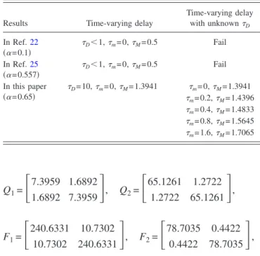
, 共14兲 fi共xi兲 = 0.5共兩xi+ 1兩 − 兩xi− 1兩兲, i = 1,2.Applying the conditions in Theorem 1 with convergence rate ␣= 0.5 and m= 0, M=D= 1.5, a feasible solution is
given by = 54.6014, = 14.2029, P =
冋
125.4731 11.3513 11.3513 125.4731册
, R1=冋
209.9502 − 18.2986 − 18.2986 209.9502册
, R2=冋
104.5948 6.4486 6.4486 104.5948册
,Q1=
冋
7.3959 1.6892 1.6892 7.3959册
, Q2=冋
65.1261 1.2722 1.2722 65.1261册
, F1=冋
240.6331 10.7302 10.7302 240.6331册
, F2=冋
78.7035 0.4422 0.4422 78.7035册
, F3=冋
− 50.0202 − 0.6362 − 0.6362 − 50.0202册
.In order to show the significant contributions of this pa-per, we summarize the comparisons between the obtained results with that of Refs.22and25in TableI.
Example 2. Consider the neural network 共2兲 associated with the following parameters, which are adopted from Ex-amples 1 and 2 of Refs.21and24.
Example 1 of Ref.21: C =
冋
1 0 0 1册
, A =冋
− 0.1 0.3 0 − 0.1册
, 共15兲 B =冋
0.5 0.4 0.15 0.5册
, ⌺ =冋
0.1 0 0 0.1册
. Example 2 of Ref.21: C =冋
1 0 0 1册
, A =冋
− 0.25 0.3 0.15 − 0.25册
, 共16兲 B =冋
0.25 0.3 0.15 0.25册
, ⌺ =冋
0.1 0 0 0.1册
.Some comparisons on upper bounds of time delay guar-anteeing the global exponential stability of these systems are made in TableII.
From the above comparisons, we conclude that the ob-tained results are less conservative than those derived in ex-isting results.
IV. CONCLUSIONS
In this paper, several sufficient conditions guaranteeing the globally exponential stability for neural networks with interval time-varying delays have been proposed. Delay-dependent criteria have been derived to guarantee the expo-nential stability of the considered neural networks. From the numerical comparisons, significant improvements over the recent existing results have been observed.
1L. O. Chua and L. Yang, IEEE Trans. Circuits Syst. 35, 1257共1988兲. 2L. O. Chua and T. Roska, Cellular Neural Networks and Visual Computing
9共Cambridge University Press, Cambridge, 2002兲.
3T. Roska and L. O. Chua, Int. J. Circuit Theory Appl. 20, 469共1992兲. 4T. Roska, C. W. Wu, M. Balsi, and L. O. Chua, IEEE Trans. Circuits Syst.,
I: Fundam. Theory Appl. 39, 487共1992兲.
5J. Cao and D. Zhou, Neural Networks 11, 1601共1998兲.
6S. Arik and V. Tavsanoglu, IEEE Trans. Circuits Syst., I: Fundam. Theory Appl. 47, 571共2000兲.
7V. Singh, IEE Proc.: Control Theory Appl. 151, 125共2004兲. 8V. Singh, Electron. Lett. 40, 9共2004兲.
9V. Singh, IEEE Trans. Neural Netw. 15, 223共2004兲. 10M. Dong, Phys. Lett. A 300, 49共2002兲.
11J. Cao, Phys. Lett. A 267, 312共2000兲. 12Z. Gui and W. Ge, Chaos 16, 033116共2006兲.
13B. Liu and L. Huang, Chaos, Solitons Fractals 32, 617共2007兲. 14C. M. Marcus and R. M. Westervelt, Phys. Rev. A 39, 347共1989兲. 15P. Baldi and A. F. Atiya, IEEE Trans. Neural Netw. 5, 612共1994兲. 16K. Gopalsamy and X. He, Physica D 76, 344共1994兲.
17Y. J. Cao and Q. H. Wu, IEEE Trans. Neural Netw. 7, 1533共1996兲. 18X. S. Yang and Y. Huang, Chaos 16, 033114共2006兲.
19L. Wang and X. Zou, Neural Networks 15, 415共2002兲.
20W. Wang and J. Cao, IEE Proc.: Control Theory Appl. 153, 397共2006兲. TABLE I. Comparisons for some bounds of time delay that guarantee the
exponential stability of system共14兲共Example 1兲.
Results Time-varying delay
Time-varying delay with unknownD In Ref.22 共␣= 0.1兲 D⬍1,m= 0,M= 0.5 Fail In Ref.25 共␣= 0.557兲 D⬍1,m= 0,M= 0.5 Fail In this paper 共␣= 0.65兲 D= 10,m= 0,M= 1.3941 m= 0,M= 1.3941 m= 0.2,M= 1.4396 m= 0.4,M= 1.4833 m= 0.8,M= 1.5645 m= 1.6,M= 1.7065
TABLE II. Comparisons of the upper bounds of time delay for Example 2. Some bounds of time delay that guarantee the exponential stability of sys-tem共15兲
Results Time-varying delay
Time-varying delay with unknownD In Ref.21 D⬍1,m= 0,M= 0.3623 Fail In Ref.24 共␣= 0.7437兲 D⬍1,m= 0,M= 1 Fail In this paper 共Remark 3兲 D = 5,m= 0,M= 12.6426 m= 0,M= 12.6426 m= 0.5,M= 13.0907 m= 1,M= 13.5907 m= 5.5,M= 18.0907 m= 12,M= 24.5907 In this paper 共␣= 0.8兲 D= 5,m= 0,M= 2.0500 m= 0,M= 2.0500 m= 0.5,M= 2.1464 m= 1,M= 2.2379 m= 1.5,M= 2.3246 m= 2,M= 2.4084 Some bounds of time delay that guarantee the exponential stability of system共16兲 In Ref.21 D⬍1,m= 0,M= 1.5947 Fail In Ref.24 共␣= 0.3958兲 D⬍1,m= 0,M= 4 Fail In this paper 共Remark 3兲 D = 10,m= 0,M= 20.5690 m= 0,M= 20.5690 m= 0.5,M= 21.0348 m= 1,M= 21.5348 m= 4,M= 24.5348 m= 8.5,M= 29.0348 In this paper 共␣= 0.4兲 D= 10,m= 0,M= 4.0414 m= 0,M= 4.0414 m= 0.5,M= 4.1345 m= 1,M= 4.2821 m= 2,M= 4.6634 m= 3.5,M= 5.2838 m= 5,M= 5.9025
21G. J. Yu, C. Y. Lu, J. S. H. Tsai, T. J. Su, and B. D. Liu, IEEE Trans. Circuits Syst., I: Fundam. Theory Appl. 50, 677共2003兲.
22Q. Zhang, X. Wei, and J. Xu, Chaos, Solitons Fractals 23, 1363共2005兲. 23S. Arik, Neural Networks 17, 1027共2004兲.
24T. L. Liao, J. J. Yan, C. J. Cheng, and C. C. Hwang, Phys. Lett. A 339, 333共2005兲.
25J. H. Park, Appl. Math. Comput. 183, 1214共2006兲. 26V. Singh, Chaos, Solitons Fractals 32, 609共2007兲. 27J. Cao and J. Liang, J. Math. Anal. Appl. 296, 665共2004兲. 28Z. Liu and L. Liao, J. Math. Anal. Appl. 290, 247共2004兲.
29X. Liao, G. Chen, and E. N. Sanchez, IEEE Trans. Circuits Syst., I:
Fun-dam. Theory Appl. 49, 1033共2002兲.
30T. Ensari and S. Arik, IEEE Trans. Autom. Control 50, 1781共2005兲. 31T. Ensari and S. Arik, IEEE Trans. Circuits Syst., I: Fundam. Theory Appl.
52, 126共2005兲.
32J. Cao, K. Yuan, and H. X. Li, IEEE Trans. Neural Netw. 17, 1646共2006兲. 33D. Yue, Q. L. Han, and C. Peng, IEEE Trans. Circuits Syst., I: Fundam.
Theory Appl. 51, 640共2004兲.
34X. Jiang and Q. L. Han, Automatica 41, 2099共2005兲. 35X. Jiang and Q. L. Han, Automatica 42, 1059共2006兲. 36E. Tian and P. A. Peng, Fuzzy Sets Syst. 157, 544共2006兲.