行政院國家科學委員會專題研究計畫成果報告
利用階層式時-空拆解法的多重參數估量極其在信號處理及無線 通訊的應用
Joint Parameter Estimation via Hierarchical Space-Time Decomposition in signal Processing and Wireless Communication
計畫編號: NSC 96-2221-E-011-012 執行期限:96/08/01 - 97/07/31 國立臺灣科技大學電子系 主持人:方文賢
計畫參與人員: 林俊宏、黃家成、陳冠宇、彭建榮
一、 中文摘要
本計畫發展一種基於平面天線陣列的階層式時 -空拆解(HSTD)之快速演算法則,可同時估測通訊 系統中信號進入之二維方位角和載波頻率等重要參 數。基於 HSTD 階層樹狀之架構下,此演算法交錯 運用一連串一維正么信號參數轉置恆定估測技術 (Unitary- ESPRIT)進行參數估測,在每一 Unitary- ESPRIT 運用前,透過時域濾波及空間波束組合等 步驟,將信號進行較佳化的分群,藉以提高參數估 測之正確性,同時抑制雜訊對估測之干擾。此外,
各參數在估量的過程中,將可自動完成配對,無需 額外的計算。模擬結果驗證,本計畫所發展之演算 法在達到既有演算法相同性能下,可有效降低原有 演算之計算複雜度。
關鍵詞︰二維方位角估測,陣列信號處理,多維度 信號處理
Abstract
In this project, we develop a fast algorithm for joint estimation of the azimuth and elevation angles, and frequencies of the incoming signals using a hierarchical space-time decomposition (HSTD) technique. Based on the HSTD, the proposed algorithm makes use of a sequence of one-dimensional (1-D) Unitary Estimation of Signal Parameters via Rotational Invariance Techniques (ESPRIT) algorithms to estimate these parameters alternatively in a hierarchical tree structure. Also, in between every
other 1-D Unitary ESPRIT, a temporal filtering process or a spatial beamforming process is invoked to partition the signals into finer groups to enhance the estimation accuracy and to alleviate the contaminated noise. Furthermore, the pairing of these parameters is automatically determined. Simulation results show that the new algorithm provides satisfactory performance but with drastically reduced computations compared with previous works. Simulation results show that the new algorithm provides satisfactory performance but with drastically reduced computations compared with previous works.
Keywords: 2-D DOA Estimation, array signal processing, multidimensional signal processing 二、 計畫緣由與目的
Joint estimation of azimuth and elevation angles, and carrier frequencies of multiple sources is of importance in wireless communications. For example, these parameters can be applied to locating the mobiles and to allocating pilot tones in space division multiple access systems [1]. Also, a precise estimation of these parameters is helpful in obtaining a better channel estimate and thus enhances the system performance. Therefore, joint estimation of these parameters has received lots of attention recently.
Various higher-dimensional subspace based algorithms such as Multiple Signal Classification (MUSIC) [2] or ESPRIT [3]-based algorithms have
been reported to jointly estimate these three parameters. The latter are in particular computationally attractive, as they are free of higher-dimensional search on the azimuth-elevation frequency plane. For example, Haardt et al. [1]
addressed a 3- D unitary-ESPRIT to estimate these three parameters by extending the computationally efficient 1-D Unitary ESPRIT to 3-D scenarios.
Strobach [4] incorporated a total least squares phased averaging method in the 3-D ESPRIT for signal subspace estimates to increase the estimation accuracy.
Despite the effectiveness of [1, 4], they call for high computational overhead due to higher-dimensional data stacking and eigendecomposition. On the other hand, an efficient ESPRIT algorithm was recently considered in [5], which, however, needs special antenna array geometry.
In order to yield high estimation accuracy with low computational complexity, this paper proposes an HSTD-based algorithm for joint estimation of the azimuth and elevation angles, and frequencies of the incoming signals. The essence of the proposed algorithm lies in a succinct combination of the parameter estimation and temporal filtering/spatial beamforming processes, in which the parameters are estimated alternatively in a hierarchical tree structure.
More specifically, the proposed algorithm makes use of a sequence of 1-D Unitary ESPRIT algorithms to estimate these parameters in a coarse-fine manner. In addition, to enhance the estimation accuracy, in between every other 1-D ESPRIT algorithm, a temporal filtering process or a spatial beamforming process is invoked to partition the incoming signals into finer groups. Based on such an HSTD technique, not only the estimation accuracy is enhanced, but the pairing of these parameters is automatically achieved without extra computations. Simulation results show that the new algorithm provides satisfactory performance but with drastically reduced computations compared with previous works.
三、 研究方法及成果 Data Model
Consider a uniform rectangular array (URA) with M × N omni-directional antennas. Assume that there are K uncorrelated narrowband sources { ( )}s tk , each of which is carried by the frequency fk, impinging on the URA, where each antenna is followed by a tapped delay line with L time delay elements of delay Ts, as shown in Fig.1.
By sampling the output of each antenna at a rate fs =1/Ts, the observed signal at time t at the lth delay element output of the (m,n)th antenna element can be expressed as
1 1
2 ( ) 2 ( )
2 2
1
2 ( 1 )
2
( ) ( )[ , ,...,
] ( ), (1)
k k
k s
M N
K j m u j n v
mnl k
k
j L l f T
mnl
x t s t e e
e n t
π π
π
− −
− − − −
=
− −−
=
+
∑
where uk d fksin kcos k
c φ θ
= and
k k
v d f
= c ⋅ sinφksinθk in which φk and θk are the elevation and azimuth angles of the kth signal, respectively, c is the wave propagation speed, and d is the antenna spacing which is equal to half of the wavelength. nmnl(t) denotes the white noise with power σn2 at the lth delay element of the (m,n)th antenna. Note that for the employment of the Unitary ESPRIT, the reference point is set at the center of the URA and, without loss of generality, M N, and L are all assumed to be even.
PROPOSED FAST ALGORITHM:
The proposed algorithm begins with the estimation of the frequencies of the incoming signals, as in general we have more temporal data to render a precise frequency estimate. To achieve this, we first construct Xf( )t by stacking xmnl( )t as
11 1 1
( ) [ ( ), , ( ) , ( ), , ( )]
f t = w t L wM t MLM w N t L wMN t
X x x x x (2)
where xwmn( )t =[xmn1( ),t L,xmnL( )]t , m =1,…,M, n = 1,…,N. Based on (1), it can be readily shown that
1
( ) ( ) ( ) ( )
K
T
f k k k k f
k
t s t t
=
=∑ ⊗ +
X g v u N (3)
where
1 1
2 2
2 2
[ k s, , k s]
L L
j f T j f T
T
k e π e π
− −
= − L
g ,
2 1
[ 2 k
j M u
k e π
− −
= u
2 1
, , 2 k]
j M u T
e π
−
L ,
1 1
2 2
2 2
[ k, , k]
N N
j v j v T
k e π e π
− −
= − L
v ,
and ⊗ denote the Kronecker product [6]. Also, the noise matrix Nf( )t is constructed by {nmnl( )}t in the same way as Xf( )t from {xmnl( )}t given in (2).
We then consider the frequency covariance matrix of Xf( )t , 1
[ ( ) H( )]
f E f t f t
=MN
R X X , with
( )⋅ H being the Hermitian operation. Based on (3), R can be shown as f
2 H
f = +σn
R GΛG I (4)
where we have the fact that (vk⊗uk) (T vk ⊗uk)*
=MN [6], and that the noise nmnl( )t is white and independent with the impinging signals.
[ ,...,1 K]
=
G g g is the frequency signature matrix and Λ=E[ ( )S St H( )]t , in which
( )t =diag s t{ ( ),...,1 sK( )}t
S . Note that R and G f
share the same column space and thus the 1-D Unitary ESPRIT can be employed to estimate the frequencies.
However, the Unitary ESPRIT can not well resolve closely spaced parameters [7], as the related signature matrix tends to be ill-conditioned. To overcome this setback, we employ the HSTD technique [8, 9] to partition the signals into smaller groups based on the resolvable carrier frequencies estimated above before proceeding to estimate u and v.
To achieve this, suppose that after carrying out the 1-D Unitary ESPRIT with respect to R , we obtain a set f of estimates of frequency estimates, say, { ,...,fˆ1 fˆq}, where q is the number of resolvable frequencies, we construct a set of temporal projection matrices
fi
P given by
( ) 1
i
H H
f i i i i
= − −
P I G G G G (5) for i=1,…,q, where Gi =[g g gˆ1,...,ˆ ˆi, i+1,...,gˆq]. We then use these projection matrices to obtain the filtered data matrices ( ) ( )
i i
f t = f f t
X P X , i=1,…,q, which, based on the data model in (3), can be re-written as.
, , , ,
1
( ) ( ) ( ) ( )
i
i i
r
T
f i j i j i j i j f f
j
t s t t
=
≅∑ ⊗ +
X g v u P N (6)
where ri is the number of signals in the ith group,
, i ,
i j = f i j
g P g . Note that the incoming sources except those in the ith group will be approximately annihilated by such a temporal filtering process. And that the filtered data matrix only contains signals whose frequencies are close to ˆ
fi but with diverse (u,v)’s.
Next, in order to estimate u by using the 1-D Unitary ESPRIT with the filtered data matrix, we partition ( )
fi t
X into a set of L×M sub-block matrices and then rebuild them into ( )
ui t X as
( ) [ ( )(:,1: ) ( )(:, ( 1) 1: ) ]
i i i
T T
u t = f t M MLM f t N− M+ NM
X X X
(7) Based on (7), it can be readily shown that ( )
ui t X renders
, , , ,
1
( ) ( ) ( ) ( )
i
i i
r
T
u i j i j i j i j u
j
t s t t
=
=∑ ⊗ +
X u v g N (8)
Where ( )
ui t
N is constructed ( )
fi f t
P N in the same way as (7), whose covariance matrix is given by
[ ( ) ( )] 2
i i i
H
u u n
E N t N t =σ I (9)
where 2 1 2
ni n
L q
σ = − +L σ , which implies that the noise components in ( )
ui t
N remains to be white and that the noise power is reduced after the filtering process.
Next, we compute the covariance matrices of
i( )
u t
X , 1
[ ( ) ( )]
i i i
H
u E u t u t
= LN
R X X . Based on (8), it can be shown that
2
i i
H
u = i i i +σn
R U Λ U I (10) where we have used the fact that
*
, , , ,
(vi j⊗gi j) (T vi j⊗gi j) =LN. [ ,1,..., , ]
i= i i ri
U u u is
the signature matrix of u and i j, Λi=E[ ( )Si t SiH( )]t , in which ( ) { ,1( ),..., , ( )}
i t =diag si t si ri t
S . Carrying out
the 1-D unitary ESPRIT, we can get a set of estimates of u, say, u , i = 1,…,q, j =1,…,rˆi j, j. Thereafter, we use these estimates to construct a set of spatial projection matrices given by
,
1
, ( , ) ,
i j
H H
u i j i j i i j
= − −
P I U U U U (11)
for i = 1,…,q, j =1,…,rj and Ui j, =[uˆi,1,...,uˆi j−, 1,
, 1,..., ,
ˆ ˆ ]
i j+ i ri
u u . Pre-multiplying data ( )
ui t X by
,
ui j
P yields a set of finer group of data as
,
, , , , , , , , , , ,
1
( ) ( ) ( ) ( )
i j
i j i j i j
z
T
u i j l i j l i j l i j l u u
l
t s t t
=
≅∑ ⊗ +
X u v g P N (12)
where z is the number of signals in the ji j, th subgroup of the ith group and
, , i j, , ,
i j l = u i j l
u P u . Note that the incoming rays, except those in the (i, j)th groups, will be approximately eliminated by
,
ui j
P .
Note that the incoming signals in the (i, j)th subgroup, which posses close u components (close to ui,j), will have diverse v’s. As such, the v components for the signals in each subgroup can be well resolved.
To estimate v, we stack the filtered matrix
, ( )
ui j t X by
, ,
,
( ) [ ( ( )(:,1: ) )
( ( )(:, ( 1) 1: ) )]
i j i j
i j
T
v u
T T
u
t vec t L
vec t N L NL
=
− +
X X MLM
X (13)
where vec( )⋅ denotes vector stacking operation [6].
Based on (13), it can be shown that
, ( )
vi j t
X renders
,
, , , , , , , , , ,
1
( ) ( ) ( ) ( )
i j
i j i j
T
v i j l i j l i j l i j l v
l
t s t t
ρ
=
≅∑ ⊗ +
X v u g N (14)
where
, ( )
vi j t
N is obtained from
, , , ( )
i j i j l
u t
P u in the same way as (13). Next, we determine the covariance matrix of
, ( )
vi j t X ,
, , ,
1 [ ( ) ( )]
i j i j i j
H
v E v t v t
= LM
R X X .
Based on (14), it can be shown that
,
2
, , , ,
i j
H v ≅ i j i j i j+σi j
R V Λ V I (15)
where 2 2
,
( 1)( i 1)
i j n
L q M r σ = − +LM − + σ ,
, [ , ,1,..., , , , ]
i j = i j i j zi j
V v v
is the signature matrix of vi j l, , , and Λi j, =E[S Si j, Hi j, ], in which
, ( ) { , ,1( ),..., , , , ( )}
i j t =diag si j t si j zi j t
S . Along the
same line as above, the 1-D Unitary ESPRIT can be applied to estimate v.
Note that the f’s and u’s estimated above are rather rough when these parameters are closely spaced.
Consequently, we can get a more precise estimate of f’s and u’s by carrying out the 1-D Unitary ESPRIT again based on the finer groups of data. For this, we construct another set of spatial projection matrices given by
, ,
1
, , ( , , , , ) , ,
i j l
H H
v i j l i j l i j l i j l
= − −
P I V V V V (16)
where
, , [ˆ , ,1 ˆ , , 1 ˆ , , 1 ˆ , , , ]
i j l = i j L i j l− i j l+ L i j zi j
V v v v v , and
then premultiply
, ( )
vi j t
X by the projection matrix
, , i j l
Pv to render
, , ( ) , , , ( )
i j l i j l i j
v t = v v t
X P X , which will
annihilate the impinging signals those do not belong to the (i, j, l)th subgroup. Based on (13), the new data matrix can be expressed as
, ,( ) , , ( ) , ,( , , , ,) , , ( )
i j l i j l
T
v t ≅si j l t i j l i j l⊗ i j l + v t
X v u g N (17)
where
, , , , , ,
i j l i j l
v = v i j l
v P v and
, , ( ) , , , ( )
i j l i j l i j
v t = v v t
N P N .
For a more accurate estimation of f, we partition
, , ( )
i j l
v t
X into M N×L sub-block matrices and stack them as
, , ,
, ,
, , , , , , , , , ,
( ) [ ( ( )(:,1: ) )
( ( )(:, ( 1) 1: ) )]
( ) ( ) ( )
i j i j l
i j l
i j l
T
u v
T T
v
T
i j l i j l i j l i j l u
t vec t L
vec t M L ML
s t t
=
− +
= ⊗ +
X X MLM
X
u v g N
(18)
where
, , ( )
i j l
Nu t is obtained from
, , ( )
i j l
Nv t in the same way as
, , ( )
i j l
u t
X from
, , ( )
i j l
v t
X in (18). Next, we partition the data matrix
, , ( )
i j l
v t
X into N M×L sub-block matrices and stack them as
, , ,
, ,
, , , , , , , , , ,
( ) [ ( ( )(:,1: ) )
( ( )(:, ( 1) 1: ) )]
( ) ( ) ( )
i j i j l
i j l
i j l
T
v v
T T
v
T
i j l i j l i j l i j l v
t vec t L
vec t M L ML
s t t
=
− +
= ⊗ +
X X MLM
X
u v g N
(19)
Note that gi j l, , in (19) does not possess the Vander- monde structure. To overcome this setback, we utilize the fact that gi j l, ,(vi j l, , ⊗ui j l, , )T belongs to the subspace spanned by the normalized eigenvector
, , i j l
ef
associate with the largest eigenvalue of covariance matrix
, , i j l
Rf , where
, , , , , ,
1 [ ( ) ( )]
i j l i j l i j l
H
f E f t f t
=MN
R X X .
Therefore,
, , , , , , , , , ,
( ) ( )
i j l i j l i
H T
f f f i j l i j l i j l
− ⊗ =
I e e P g u v 0
belongs to the subspace spanned by
, , i j l
Ξf =
, , , ,
( )
i j l i j l i
H
f f f
− −
I I e e P . Denote Gi j l, , =[G gi i j l, , ], then it can be shown that
, ,
1
, ,( , , , ,) , ,
i j l
H H
f i j l i j l i j l i j l
Ξ = G G G − G (20)
Note that Gi j l, , retains the Vandermonde structure and shares the same column space as
, , i j l
Ξf , so the 1-D Unitary F-ESPRIT can be utilized and we can get more precise estimates of f’s. Similarly, working with
, , i j l
Xu results in more precise estimates of ui,j,l’s.
To sum up, the overall steps of the proposed tree-structured 1-D Unitary ESPRIT based algorithm can be summarized as follows:
Step 1: (Rough Frequency Estimation) Estimate the covariance matrix
1
ˆ 1 ( ) ( )
S
H
f f s f s
s
t t
SMN =
= ∑
R X X where
S is the number of snapshots, and then invoke the 1-D Unitary ESPRIT to yield a set of group frequency estimates { ,...,fˆ1 fˆq}, where q is the number of resolvable frequencies.
Step 2: (Temporal Filtering) Employ { ,...,fˆ1 fˆq} to construct the projection matrix
fi
P by (5) and then use Pfi to obtain the filtered data matrix ( )
fi t = X
i ( )
f f t
P X , i = 1,…, q.
Step 3: (Rough Estimation of u) Stack the data
i( )
f t
X , i = 1,…, q, based on (6) and then estimate the covariance matrix
1
ˆ 1 ( ) ( )
i i i
S
H
u u s u s
s
t t
SLN =
= ∑
R X X .
Thereafter, use the 1-D Unitary ESPRIT to estimate the u’s,
1,1 1,1 ,1 ,
ˆ ˆ ˆ ˆ
{ ,..., ,..., ,..., }
r q q rq
u u u u , where ri; i = 1,…, q, is the number of u’s resolvable in the ith group.
Step 4: (Spatial Beamforming (I)) Employ {uˆi j, } obtained above to construct the projection matrix
,
ui j
P by (11) and then use
,
ui j
P to obtain the filtered data matrix
, ( ) , ( )
i j i j i
u t = u u t
X P X , i=1,…,q, j=1,…,rq. Step 5: (Estimation of v) Re-stack data
, ( )
ui j t X based on (13) to form
, ( )
vi j t
X and then use
, ( )
vi j t X to estimate the covariance matrix
,
ˆ 1
vi j
= SLM R
, ,
1
( ) ( )
i j i j
S
H
v s v s
s
t t
∑= X X . Thereafter, use the 1-D Unitary ESPRIT to estimate the v’s to get {vˆi j l, ,}.
Step 6: (Spatial Beamforming (II)) Employ {vˆi j l, ,} to construct the projection matrices
, , i j l
Pv as given in
(16), then use
, , i j l
Pv to obtain filtered data matrix
, , ( ) , , , ( )
i j l i j l i j
v t = v v t
X P X , i =1,…,q, j=1,…,rq, l=1,…, zi,j.
Step 7: (Precise u and Frequency Estimation) Partition and restack
, , ( )
i j l
v ts
X as (18) and (19) to obtain
, , ( )
i j l
u ts
X and
, , ( )
i j l
f ts
X , respectively.
Estimate the covariance matrix
, ,
ˆ 1
i j l
f = SMN
R
, , , ,
1
( ) ( )
i j l i j l
S
H
f s f s
s
t t
∑= X X , and utilize the normalized eigenvector
ˆ , , i j l
ef corresponding to the largest eigenvalue and the projection matrix
fi
P to form
, , ( , , , , )
i j l i j l i j l i
H
f f f f
Ξ = − −I I e e P . Use the 1-D Unitary ESPRIT to obtain precise frequency estimates from
, , i j l
Ξf . Following the above procedures based on
, , ( )
i j l
u ts
X renders precise estimates of u. Note that since every subgroup in this step only contains one signal, the pairing process is automatically achieved.
Finally, we can obtain the estimate of elevation and azimuth angles, ˆ sin 1 ˆ2 ˆ2
ˆ
c u v
φ = − fd + and
1 ˆ ˆ tan
ˆ v θ= − u.
Note that the number of groups, q, the number of signals in each group, ri, and the number of signals in each subgroup, zi,j are known or have been perfectly estimated, say by the AIC or MDL criterion addressed in [10]. Based on the above steps, the total number of real multiplications required by the proposed algorithm is then about 4LMNSK(L+M+N) if we assume that S≥M N L, , >K.
Simulations and Discussions
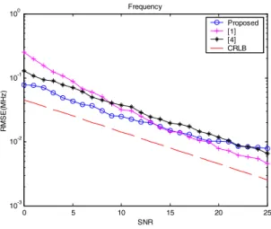
Some simulations are conducted in this section to assess the proposed approach. Assume that there are K
= 4 users, and they are received by a 6×6 (M = N = 6) element URA which spaced a half wavelength apart, where each antenna is followed by a tapped line with L
= 12 delay elements and the sampling frequency is fs = 400 MHz. The azimuth and elevation angles of the users are [63; 29; 75; 63]o and [23; 44; 46; 13]o,
respectively, with the center frequencies [100; 103;
103; 180] MHz. S = 200 symbols are employed to estimate the temporal and spatial covariance matrices.
For each specific SNR, 200 Monte Carlo trials are carried out. The comparison of the root-mean-square-error (RMSE) of frequencies, elevation and azimuth angles based on the proposed algorithm and [1] and [4] is shown in Figs. 3, 4 and 5, respectively, where the Cramer-Rao lower bound (CRLB) is also provided for reference.
We can note from Figs. 3-5 that the proposed algorithm produces close performance as the algorithms in [1, 4] in all of the estimates. Meanwhile, [1] and [4] need to stack the data to simultaneously estimate these parameters and thus roughly require (6S +2/3MNL)M2N2L2 and (8S+8/3MNL+34K)M2N2L2 real multiplications, respectively, which are far more computationally expensive than the proposed algorithm. In contrast, the proposed algorithm only involves 1-D unitary ESPRIT and thus the computational overhead is substantially reduced.
四、 計畫成果自評
Compared with current estimation algorithms for joint estimations of the 2-D DOAs and carrier frequencies in existing literature, the proposed algorithms possess the following attractive attributes: (1) it only employes the 1-D Unitrary ESPRIT to estimate these three parameters, so the computation complexity is substantially reduced; (2) the pairing of parameters is automatically reached without extra complexity; (3) With the ingenious incorporation of the temporal filtering and spatial beamforming processes, the noise power is reduced which results in enhanced estimation accuracy. Simulation results are also furnished to justify the proposed approach. This research result has been submitted to Signal Processing and is currently under the review process.
Right now, we are working on the extension of this HSTD technique to other similar signal processing or
communication problems
五、 參考文獻
[1] M. Haardt and J. A. Nossek, ”3-D unitary ESPRIT for joint 2-D angle and carrier estimation,” in Proc.
IEEE Int’l Conf., Acoustics, Speech, and Signal Processing, pp. 255-258, 1997.
[2] R. O. Schmidt, “Multiple emitter location and signal parameter estimation,” in Proc. RADC Spectral Estimation Workshop, pp. 243-258, Rome, NY. 1979.
[3] R. Roy and T. Kailath, “ESPRIT-Estimation of signal parameters via rotational invariance techniques,” IEEE Tran. ASSP, vol. 37, pp.
984-995, July 1989.
[4] P. Strobach, “Total least squares phased averaging and 3-D ESPRIT for joint azimuth-elevation-carrier estimation,” IEEE Tran.
Signal Processing, vol. 49, pp. 54-62, Jan. 2001.
[5] C.-Y. Qi, Y.-L.Wang, Y.-S. Zhang and H. Chen,
“A space-time processing approach to joint estimation of signal frequency and 2-D direction of arrival,” in Proc. IEEE AP-S/URSI, vol. 3A, pp.
370-373, 2005.
[6] G. H. Golub and C. F. Van Loan, Matrix Computations. 3rd ed. Johns Hopkins University Press, 1996.
[7] A. N. Lemma, A.-J. van der Veen, and E. F.
Deprettere, “Analysis of joint angle-frequency estimation using ESPRIT,” IEEE Trans. Signal Processing, vol. 51, pp. 1264-1283, May 2003.
[8] Y.-Y. Wang, J.-T. Chen, and W.-H. Fang,
“TST-MUSIC for joint DOA-delay estimation,”
IEEE Trans. Signal Processing, vol. 46, no. 4, pp.
721-729, Apr. 2001.
[9] J.-D. Lin, W.-H. Fang, Y.-Y. Wang, and J.-T. Chen,
“FSF MUSIC for joint DOA and frequency estimation and its performance analysis,” IEEE Trans. Signal Processing, vol. 54, no. 12, pp.